Development of a Statistical Shape-Function Model of the Implanted Knee for Real-Time Prediction of Joint Mechanics

IMPLANTED KNEE FOR REAL-TIME PREDICTION OF JOINT MECHANICS

by Kalin Gibbons

A thesis

submitted in partial fulfillment of the requirements for the degree of Master of Science in Mechanical Engineering

Boise State University

DEFENSE COMMITTEE AND FINAL READING APPROVALS

of the thesis submitted by

Kalin Gibbons

Thesis Title: Development of a Statistical Shape-function Model of the Implanted Knee for Real-time Prediction of Joint Mechanics

Date of Final Oral Examination: 07 June 2019

The following individuals read and discussed the thesis submitted by student Kalin Gibbons, and they evaluated his presentation and response to questions during the final oral examination. They found that the student passed the final oral examination.

Clare Fitzpatrick, Ph.D. Chair, Supervisory Committee

Trevor Lujan, Ph.D. Member, Supervisory Committee

Gunes Uzer, Ph.D. Member, Supervisory Committee

iv

v

Firstly, I would like to thank my advisor, Dr. Clare Fitzpatrick, for allowing me the opportunity to perform research within a field which I was wholly unfamiliar. She has a preternatural knack for leading us students into well-suited projects, demonstrating care with every nuanced word of guidance or criticisms she offers. I would be much less eager to continue onward to a PhD without such a wonderful advisor, and her character should be a lesson to professors the world over.

I would like to express my appreciation of Drs. Trevor Lujan and Gunes Uzer for being on my thesis committee, who are very adept at asking questions that cause me a great deal of effort to answer, but make the resulting works ten-fold more compelling. This thesis is stronger because of your guidance, and I am more prepared for the work yet to come.

Going further back, I would like to thank Dr. Krishna Pakala and Matt Schmasow, who gave me my first opportunity as a learning assistant, and taught me the interpersonal and leadership skills that have allowed me to thrive as a graduate student. Without that opportunity, undergraduate life would have continued being much lonelier. Working with these two left me fully engaged with my engineering peers and my studies, illuminating the path forward to graduate school.

vi

vii

viii

Dedication ... iv

Acknowledgments ... v

Abstract ...vii

List of Tables ...xii

List of Figures ... xiv

List of Abbreviations ... xx

Introduction ... 1

1.1 The Knee ... 2

1.2 Osteoarthritis ... 4

1.2.1 Patients ... 5

1.2.2 Treatments ... 6

1.3 Thesis Statement ... 13

1.4 Works Published ... 16

Literature Review ... 17

2.1 Clinical Trials ... 20

2.1.1 Governing Regulations... 20

2.1.2 Clinical Trial Process ... 22

2.2 Mechanical Joint Simulators (Cadaveric Knee Simulators) ... 23

ix

3.1 Finite Element Methods ... 28

3.1.1 Advantages of FEM ... 29

3.1.2 Disadvantages of FEM ... 29

3.2 Shape Function Models ... 30

3.3 Experimental Design ... 32

3.3.1 Sampling Methods ... 33

3.3.2 Regression Analysis ... 36

3.3.3 Predictor Order ... 37

3.3.4 Factor Effect Screening ... 40

Manuscript “Development of a Statistical Shape-Function Model of the Implanted Knee for Real-Time Prediction of Joint Mechanics” .. 41

4.1 Introduction ... 41

4.2 Methods ... 44

4.3 Results... 54

4.3.1 Patella ... 56

4.3.2 Ligament Elongation and Muscle Forces ... 57

4.3.3 Tibiofemoral Kinematics... 59

4.3.4 Tibiofemoral Joint Loads ... 59

4.3.5 Contact Mechanics ... 60

4.4 Discussion ... 61

Conclusions and Future Directions ... 65

5.1 Limitations ... 67

x

5.2.2 Additional Parameterized Joints ... 70 5.2.3 Graphical User Interface ... 72 References ... 74 Appendix A: Combined Set - Two Sample T-Test Factor Sensitivities ... A1 A.1 Tibiofemoral Contact Mechanics ... A2 A.2 Tibiofemoral Joint Loads ... A8 A.3 Tibiofemoral Kinematics ... A13 A.4 Tibiofemoral Ligaments ... A17 A.5 Patellofemoral Contact and Joint Mechanics, Kinematics, and

Ligaments

... A24

Appendix B: Design Set - Two Sample T-Test Factor Sensitivities ... B1 B.1 Tibiofemoral Contact Mechanics ... B4 B.2 Tibiofemoral Joint Loads ... B5 B.3 Tibiofemoral Kinematics ... B6 B.4 Tibiofemoral Ligaments ... B7 B.5 Patellofemoral Contact and Joint Mechanics, Kinematics, and

Ligaments

xi

xii

Table 1. Parameter ranges used in training and test data sets for design and surgical parameter sets. Implant geometry was parameterized using nine variables with ranges based on the geometric domain of commercially available TKA components. Six surgical alignment predictors were included, with ranges chosen to capture those of both mechanically and kinematically aligned knee replacements. ... 47 Table 2. Predicted outputs organized by functional groupings used in factor effect

screening. Four groups were created for the tibiofemoral joint, while a single group collected all outputs for the patellofemoral joint. ... 50 Table 3. Average normalized RMS errors for all outputs (%). Across all three

parameter sets, doubling the sample rate while using quadratic predictors with interactions reduced errors by an average of 30.1%. Further

investigation of sensitivity to predictor order was performed on the design set, due to it having the largest reduction in error with increasing order. . 54 Table 4. Significance by factor for the tibio-femoral contact mechanics group from

the combined parameter set. ... A3 Table 5. Significance by response for the tibio-femoral contact mechanics group

from the combined parameter set. ... A6 Table 6. Significance by factor for the tibio-femoral joint loads group from the

combined parameter set. ... A9 Table 7. Significance by response for the tibio-femoral joint loads group from the

combined parameter set. ... A11 Table 8. Significance by factor for the tibio-femoral kinematics group from the

combined parameter set. ... A14 Table 9. Significance by response for the tibio-femoral kinematics group from the

combined parameter set. ... A16 Table 10. Significance by factor for the tibio-femoral ligaments group from the

xiii

Table 12. Significance by factor for the patellar mechanics group from the combined parameter set. ... A25 Table 13. Significance by response for the patellar mechanics group from the

combined parameter set. ... A29 Table 14. Significance of response variables for the Cam Radius parameter. This

parameter was removed from the combined factor data set. ... B2 Table 15. Significance of response variables for the Femoral F-E alignment

xiv

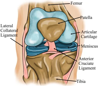
Figure 1. An overview of knee joint anatomy. The knee joint is the largest joint in the body, and any reduction in joint functionality will cause considerable burden to a person. Image adapted from (“Total Knee Replacement - OrthoInfo - AAOS,” 2019). ...2 Figure 2. Osteoarthritis is a frequently slowly progressive joint disease typically

seen in middle-aged to elderly people. In OA, the cartilage between the bones in the joint breaks down because of mechanical stress, further causing additional stress to the bones, which causes them to slowly increase in size and eventual joint failure. Image adapted from (“Total Knee Replacement - OrthoInfo - AAOS,” 2019). ...4 Figure 3. X-ray scans showing a healthy knee (left), as well as a knee suffering from bow-leg and severe OA (right). Arrows mark the deterioration of cartilage causing a loss of spacing between the bones. Image from (“Total Knee Replacement - OrthoInfo - AAOS,” 2019). ...7 Figure 4. An illustration depicting a knee afflicted with OA (left), and an implanted

joint used in total knee arthroplasty (right). Knee replacement involves resurfacing of the bones in the joint with metal components, and a friction reducing polymer spacer called the tibial insert. Image adapted from (“Total Knee Replacement - OrthoInfo - AAOS,” 2019). ...9

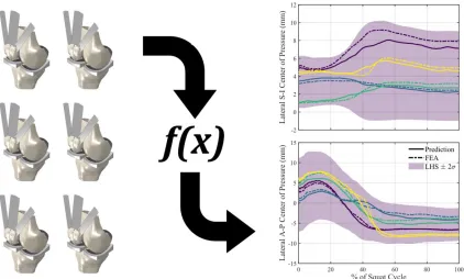
Figure 5. An infographic depicting the use of FEA simulations to train a statistical shape-function model for the instantaneous prediction of joint mechanics outputs. Once the training is completed, the prediction plots will be

generated using computationally inexpensive regression analysis. ... 13 Figure 6. An overview of the implant design process from initial planning to

xv

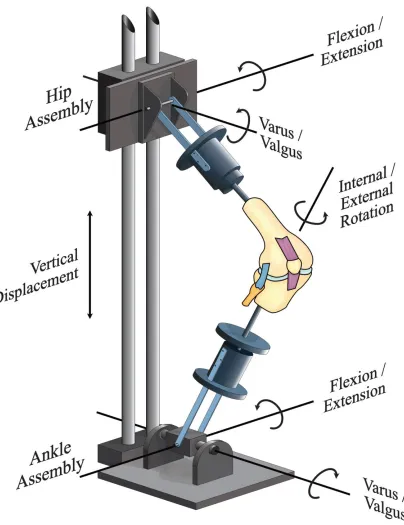
allowing specific rotations within the hip and ankle mechanism. The hip assembly is allowed motion within the flexion-extension and varus-valgus rotations, while the ankle assembly is allowed motion within the flexion-extension, varus-valgus, and internal-external tibial clinical rotations. Image adapted from (Zavatsky, 1997). ... 24 Figure 8. A knee implant design capable of telemetric measurement through usage

of four load sensors imbedded in the base of the tibial component. Image adapted from (Almouahed et al., 2017). ... 26 Figure 9. Factorial designs only produce good models when we can collect accurate

data, which was not possible in the case of this implant design (left), which used the tibial insert as a launch-ramp to dislocation (right). Other sampling methods do not require such a large number of samples and have a better spread throughout the design space, mitigating the loss of

accuracy when missing a single data point. ... 33 Figure 10. An example of a full factorial (left) and central composite (right) design

spaces for an experiment with three factors. A full factorial design

includes every combination of factors set to high and low levels, encoded to be ±1. To extend a factorial design with 𝑘 factors into a central

composite design, we add additional “star points” at a distance ±2𝑘/4 away from the mean factor value. In two and three dimensions, these additional points will circumscribe a circle or sphere with the original points. ... 34 Figure 11. Sampling a two-factor design space using a Latin square is analogous to

placing rooks on a chessboard such that none of them are able to capture each other. One of the benefits of LHS is being able to select the number of samples independently from the number of factors; we can subdivide the chess board as little or as much as we want. ... 35 Figure 12. An example of the low and high factor groupings used when performing

xvi

anterior lateral capsule (ALC), popliteofibular ligament (PFL), postero-medial capsule (PMC), posterior capsule (PCAP), and posterior oblique structures (POL). The quadriceps muscle, which was separated into rectus femoris plus vastus intermedius (RF+VI), vastus lateralis (VL) and vastus medialis (VM) bundles, was represented by 2-D fiber-reinforced

membrane elements. Patellofemoral ligaments and patellar ligament (PL) were also included. ... 44 Figure 14. Design and surgical alignment parameters, with all surgical alignments

shown positive. Implant geometry (red) was parameterized using nine variables: femoral condyle distal, posterior and coronal radii, tibial insert anterior, posterior and coronal plane conformity, trochlear orientation and M-L position, and coronal plane curvature of the cam mechanism. Six surgical alignment predictors (black) included: tibial insert and femoral implant V-V and I-E alignment, femoral F-E alignment, and tibial insert slope, with ranges chosen to capture those of both mechanically and kinematically aligned knee replacements. ... 48 Figure 15. Pareto charts justifying the removal of femoral F-E alignment and cam

radius parameters from the combination set, developed from factor effect screening analysis for the surgical alignment (top) and design geometry (bottom) parameters. Factor effects screening was performed by dividing output results into low and high factor blocks, where each single predictor variable was categorized as low when set below its average value, and high when set above average. For every combination of output and factor, the magnitude of the difference between the high block and the low block was taken and normalized by dividing by the average. ... 51 Figure 16. Overlayed area plots of average normalized RMS error by functional

group. Within each set of parameters, highest errors are associated with linear predictors using half-sized samples, and are reduced by keeping linear predictors while doubling the sampling rate, then minimized using doubled sample rate with quadratic predictors with interaction terms. Joint loads and contact mechanics functional groups produced larger

xvii

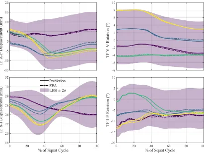
sampling of 130 simulations with linear predictors. This functional group had normalized mean RMS errors, averaged by group, below 5% across all parameter sets, with errors resulting in 1.61%, 3.30%, and 3.97% for the surgical, design, and combined sets, respectively. ... 57 Figure 18. Prediction of kinematic results from four randomly generated knees for

tibiofemoral A-P and S-I displacement, and I-E and V-V rotation of the combination parameter set using 10 simulations per parameter with linear predictors. Kinematics predictions of the TF joint resulted in normalized mean RMS errors, averaged by group, of 3.78% for the surgical, 11.3% for the design, and 10.8% for the combination parameter sets. ... 58 Figure 19. Representative contact mechanics and joint loads prediction results from

the combination set, using a sample size of 130 simulations and linear predictors for regression analysis. Four randomly generated knees were selected from each functional group. From the contact mechanics group, the surgical set had a normalized mean RMS error, averaged by group, of 7.97%, while the design set scored 15.3%, and the combination set resulted in an error of 19.2%. For the surgical set, normalized mean RMS joint load errors, averaged by group, were only 8.38%, whereas the design set resulted in an error of 14.2%, and the combined set had the largest error of 18.4% for this group. ... 60 Figure 20. Significance rankings for the tibiofemoral contact mechanics group of the

combined set. All unique response variables are captured by the femoral V-V, tibial slope, and femoral coronal radius factors. ... A2 Figure 21. Joint loads factor rankings from the combined parameter set. All unique

response variables are captured by the femoral posterior radius and V-V alignment parameters. ... A8 Figure 22. Factor significance rankings from the combined set, where the tibial slope

is the most significant factor, capturing all unique response variables by itself. ... A13 Figure 23. Combined set tibiofemoral ligament group factor rankings. Interestingly, a

xviii

unique response variables, which is likely due to the inclusion of ligament elongations and forces within this functional group... A24 Figure 25. Contact mechanics factor rankings for the design set. A maximum of 90%

of the unique response variables is captured by femoral posterior radius and tibial coronal conformity factors. The additional 10% were captured when moving to the combined set, showing that some of the response variables were more dependent on surgical alignment parameters. ... B4 Figure 26. Design set joint load factor significance rankings. Every unique response

variable is captured when including the first five factors, and tibial anterior conformity did not capture any response variables. This lack of

significance is likely due to the activity under study, as the knee will roll back during a deep-knee bend. ... B5 Figure 27. Kinematics factor significance rankings for the design set. All unique

response variables were captured by the femoral posterior radius factor, and none of them were significantly influenced by the cam radius. ... B6 Figure 28. Factor significance rankings for the tibiofemoral ligaments functional

group. Only 78% of the unique response variables were captured by the first four factors, with cam radius and femoral coronal radius proving insignificant for any of them. These results are similar to the combination factor set, though there was modest improvements when including surgical alignment parameters. ... B7 Figure 29. Patellofemoral factor significance ratings for the design set. Cam radius

and femoral coronal radius again proved insignificant, but only 81% of the unique response variables were captured by the three highest ranked factors. ... B8 Figure 30. Contact mechanics factor significance rankings for the surgical parameter

set. The femoral V-V factor captures 80% of the unique response variables within this functional group, and the remaining 20% were not captured until introducing design parameters in the combined set. ... C3 Figure 31. Joint loads factor significance rankings for the surgical set. All unique

responses were captured by the tibial I-E surgical alignment factor. ... C4 Figure 32. Surgical set factor significance rankings for the tibiofemoral kinematics

xix

captured by the first three factors. It is likely that some of the ligament response is driven by the activity under study, rather than the individual factors. ... C6 Figure 34. Factor significance rankings for the patellofemoral functional group of the

surgical set. Only 58% of the unique response variables were captured by the first five factors, suggesting that design parameters are more

xx

A-P Anterior-Posterior

ALC Anterior Lateral Capsule

CDC Centers of Disease Control and Prevention

CLT Central Limit Theorem

DKB Deep-Knee Bend

DOF Degrees of Freedom

FDA Food and Drug Administration

FE(M) Finite Element (Method)

F-E Flexion-Extension

GS Grood-Suntay

GUI Graphical User Interface

IDE Individual Device Exemption

IRB Institutional Review Board

I-E Internal-External

LCL Lateral Collateral Ligament

xxi

MCL Medial Collateral Ligament

MPOL Medial Posteromedial Capsule

M-L Medial-Lateral

NIH National Institutes of Health

NSAIDs Nonsteroidal Anti-Inflammatory Drugs

OA Osteoarthritis

PF Patellofemoral

PFL Popliteofibular Ligament -or- Patellofemoral Ligament

PI Proportional-Integrative

PL Patellar Ligament

PMA Premarket Authorization

PMC Posteromedial Capsule

PS Posterior Stabilized

Q + I Quadratic plus Interactions

RF Rectus Femorus

RMS(E) Root-Mean-Square (Error)

SFM Shape-Function Model

xxii

TKA Total Knee Arthroplasty

VI Vastus Intermedius

VL Vastus Lateralis

VM Vastus Medialis

V-V Varus-Valgus

2-D Two-Dimensional

INTRODUCTION

The American population is getting older, on average, and this is placing strain on our in-place healthcare systems. There is a shortage of primary care physicians, with 13% of Americans (44 million) residing within a county with inadequate coverage of primary care providers, defined as less than one primary care physician per 2,000 people (“Addressing the Nation’s Primary Care Shortage: Advanced Practice Clinicians and Innovative Care Delivery Models,” 2018). By the year 2030, the U.S. population is expected to increase by

being performed to combat them, we must begin by understanding the knee, and the dis-eases which affect it.

1.1 The Knee

The knee is one of the most complex joints in the body and having healthy knees is required to perform most everyday activities. The knee joint is made up of the distal end

of the femur, the proximal end of the tibia, and the patella (Figure 1). The contact surfaces of these three bones are protected by articular cartilage: a smooth, low-friction material that protects the bones and facilitates easy articulation. The menisci, C-shaped, shock ab-sorbing wedges are located between the femur and tibia, and act to cushion the joint. Joint stability is provided by large ligaments which hold the femur and tibia together, while the long quadriceps muscles give the joint its strength. The rest of the joint surfaces are covered by a thin lining which releases a fluid that lubricates the cartilage called the synovial mem-brane. This fluid filled membrane acts to reduce friction within the joint to nearly zero within the healthy knee (Basalo et al., 2007; Qian et al., 2006). All of these components work in harmony within the healthy knee, but disease or injury can disrupt their normal function, resulting in muscle weakness, reduced function, and chronic pain.

Arthritis is the most common cause of chronic knee pain and disability (Lawrence et al., 2008). There are many types of arthritis, but the types most associated with knee pain are osteoarthritis, rheumatoid arthritis, and post-traumatic arthritis.

 Osteoarthritis: This is an age-related degenerative type of arthritis caused by normal ‘wear and tear’. It typically occurs in people above the age of 50, but is increasingly occurring in younger people, also. When a patient has symptoms of osteoarthritis, the cartilage that protects the bones of the knee softens and wears away. This causes the bones to rub against each other, causing stiffness and knee pain.

 Post-traumatic arthritis: Following a serious knee injury, tears of the knee ligaments or fractures of the bones surrounding the knee may damage the articular cartilage, causing knee pain and limiting knee function.

All of the above examples share the traits of cartilage loss, have similar symptoms, and slowly worsen with time. As osteoarthritis is the most common form of arthritis (Hei-dari, 2011; Lawrence et al., 2008), the following section will look at OA in detail.

1.2 Osteoarthritis

of the cartilage, tendons and ligaments, and by bony changes of the joint, which are ac-companied by inflammation of the joint lining to various degrees (Lane et al., 2011) (Figure 2).

The patient reported symptoms of OA include:

 Joint pain and stiffness, possibly during rest as well as activity

 Knobby (lumpy) swelling at the joint

 Cracking or grinding noise with joint movement, especially when using stairs

 Decreased function and mobility of the joint

This arthritis is not limited to the knee, and also tends to occur within the hand, spine, hips, and great toe joints. According to the Johnston County Osteoarthritis Project (Murphy et al., 2008), a long-term study from the University of North Carolina and spon-sored by the Centers of Disease Control and Prevention (CDC) and National Institutes of Health (NIH), the lifetime risk of developing OA of the knee is about 46%, and the lifetime risk of developing OA of the hip is 25%. The incidence of knee OA is rising commensu-rately with population age, and it is one of the leading causes of disability in older people.

1.2.1 Patients

in patients age 50 and older, but it can occur earlier if a person has other OA risk factors, which, in addition to older age, include:

 Obesity

 Having family members with a history of OA

 Previous traumatic joint injury or repetitive use of joints

 Joint deformity such as unequal leg length, bowlegs, or knocked knees

There is no known cure for the disease, but current treatments exist which aim to reduce pain and improve function, and most importantly, to slow disease progression.

1.2.2 Treatments

Physical Measures

Weight loss and exercise are important in the treatment OA. Excess weight puts stress on a patient’s knee joints, hips, and lower back. For every 10 pounds of weight lost over 10 years, the chance of developing knee OA is reduced by up to 50% (“NIH Consen-sus Statement on Total Knee Replacement,” 2003). Exercise can improve muscle strength,

cane, can help patients to continue performing daily activities. For short term relief of OA symptoms, heat or cold therapy may help (Brosseau et al., 2003).

Drug Therapy

Surgery

For severe cases of OA, where the joint is seriously damaged, or when other ments have failed to relieve pain, or the patient has a major loss of function, surgical treat-ment becomes an option. Surgery may involve repair of the joint done through small inci-sions, known as arthroscopy (Barnes et al., 2006; Law et al., 2019). If the joint damage cannot be repaired in this way, joint replacement is the next option (Figure 4). Joint re-placement may be recommended when:

 Severe knee pain or stiffness limits the patient’s everyday activities, includ-ing walkinclud-ing, climbinclud-ing stairs, and gettinclud-ing in and out of chairs. Candidates for knee replacement may find it hard to walk more than a few blocks without significant pain and they may already be using a cane or walker

 Patients experience moderate or severe knee pain while resting, whether this occurs during the day or at night

 Chronic knee inflammation and swelling which has not shown improve-ment with rest or the administration of medications

 A patient exhibits a Knee deformity known to cause rapid OA progression, such as a bowing in or out of the knee joint

 Failure to show substantial improvement with other forms of treatment such as anti-inflammatory medications, cortisone and lubricating injections, physical therapy, or arthroscopic surgeries

The modern version of knee replacement surgery was first performed by Frank Gunston in 1968 (Shetty et al., 2003), and improvements in surgical materials and tech-niques over the past 50 years have greatly increased its safety and effectiveness. Today, total knee replacements are one of the most frequent and successful procedures in the United States. As of 2014, combined partial and total knee replacement is ranked the third most frequent operating room procedures, with more than 700,000 knee replacements per-formed each year in the United States (McDermott et al., 2017).

When performing a total knee replacement surgery, the procedure may be divided into four primary steps:

2. Resurfacing the tibio-femoral joint: The removed cartilage and bone is replaced with metal that has been shaped in order to recreate the smooth surface of the joint. These metal parts may be cemented or “press-fit” into the bone, and some materials exist which can chemically bond with existing bone

3. Resurfacing the patella: If wear is extensive, the contacting surface of the patella is resurfaced with plastic

4. Tibial spacer insertion: To prevent metal-on-metal wear, and to reduce the friction within the joint, a plastic spacer is inserted between the metal com-ponents

For 90% of people who have total knee replacement surgery, there is a reliable reduction of knee pain and a significant improvement in the ability to perform common activities of daily living, with full restoration of pre-disease joint function being the upper limit of surgical outcomes (Bade et al., 2010; “NIH Consensus Statement on Total Knee Replacement,” 2003). Most patients can expect to be able to almost fully straighten the

replaced knee and to bend the knee sufficiently for daily tasks, but kneeling is sometimes uncomfortable, although not harmful. Patients may also feel some stiffness, particularly when performing activities with excessive bending. Most people also feel or hear some clicking of the metal and plastic when using their joint. These symptoms often reduce with time, and most patients find them to be a tolerable improvement over pre-surgery function.

avoid high-impact activities for the rest of their post-surgery lives. Low-impact activities which a patient can expect to safely engage in following total knee replacement include walking, swimming, golf, driving, light hiking, biking, ballroom dancing, and other low-impact sports (Swanson et al., 2009).

Rehabilitation following total knee replacement surgery typically begins the day after surgery and, for some cases, patients may begin moving their knee on the same day as receiving surgery. Following surgery, surgeons will typically instruct patients to do the following:

 Participate in regular light exercise programs to maintain proper strength and mobility of their new knee.

 Take precautions to avoid falls and injuries

 Return for periodic follow-up appointments with the orthopaedic surgeon, generally once per year

When patients stick to this type of low-impact activity and follow their surgeon’s guide-lines, they can expect their knee replacement to last for many years. Today, over 90% of modern total knee replacements are still functioning correctly 15 years following surgery (Abdel et al., 2011).

performed annually within the United States, this works out to up to 140,000 dissatisfied patients. Improvements to implant design and surgical technique are active areas of re-search, with the goal of improving the current techniques until patient functionality can be completely restored to pre-surgery levels. The present thesis work contributes work to-wards this goal with the aim of reducing the time and expertise requirements associated with implant design through the use of finite element simulations as a training set in devel-oping a novel computational joint mechanics prediction model (Figure 5).

1.3 Thesis Statement

when developing a new implant design. However, the use of FEA still predicates consid-erable investments of time, capital, and expertise. The present thesis research aims to pro-vide a computational framework which will allow for the instantaneous prediction of im-planted knee joint mechanics in a manner that reduces the requisite knowledge and exper-tise when compared to the development of an FEA model. The specific objectives are as follows:

 Develop a set of parameterized FEA simulations of the implanted knee per-forming a deep knee bend (DKB) which may be used to train a statistical prediction model. Model parameters will include geometric factors and sur-gical alignments

 Determine sensitivity of key joint mechanics outputs, such as joint loads, contact mechanics, and kinematics of the tibiofemoral and patellofemoral joints, and ligament elongations and muscle forces, to changes in individual model parameters

 Produce a statistical model which enables the real-time prediction of the previously mentioned joint mechanics groups

 Validation of the statistical models against an additional test set of FEA simulations by quantifying the resulting errors for every joint mechanic out-put

The present thesis is organized in the following way:

each method, the process required, and the advantages and disadvantages of the technique are summarized.

Chapter 3 outlines the methods used in the statistical modeling of joint mechanics present within this study. It begins with an explanation of statistical shape functions, then continues to detail the components of experimental design including a survey of experi-mental sampling methods, a description of regression analysis and the nuances of the equa-tions used in linear regression, as well as a description of one sensitivity analysis technique: factor effects screening.

Chapter 4 includes a faithful reproduction of the authors’ manuscript, previously published in the Journal of Biomechanics. This manuscript provides a detailed summary of the development of the statistical prediction models which allow us to instantaneously predict joint mechanics outcomes before running a finite element simulation, as well as quantification of results and validations.

1.4 Works Published

The following works were published during the course of this study:

Gibbons, K.D., Clary, C.W., Rullkoetter, P.J., Fitzpatrick, C.K., 2019. Development of a statistical shape-function model of the implanted knee for real-time prediction of joint mechanics. Journal of Biomechanics 88, 55–63.

https://doi.org/10.1016/j.jbiomech.2019.03.010

LITERATURE REVIEW

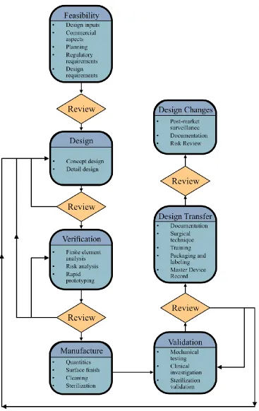
To understand the current research methodology surrounding surgical implants, it is important to first understand the implant design process. The implant design process is outlined using a series of seven steps (Figure 6):

1. Design feasibility studies

a. Planning stage where design inputs, commercial aspects, regulatory requirements, and design requirements are fleshed out

2. Design production

a. A narrowing of initial conceptual designs until a subset of one or more detailed designs are developed

3. Design verification

a. Using the most resource effective tools available to verify that the detailed design should operate as expected, satisfying the design re-quirements developed during the design feasibility stage

b. Often makes use of computational models, such as finite element methods

4. Design manufacture

a. Decisions must be made about the manufacturing methods used to produce the final products, where factors relating to this include the number to be produced, the surface finishes required, post machin-ing cleanmachin-ing processes, and any required sterilization processes

5. Design validation

a. Late stage prototypes will undergo more stringent mechanical test-ing, and possibly clinical testing as required by regulatory oversight. Sterilization processes will be tested and validated

6. Design transfer

a. Documentation and necessary clinical training protocols must be produced, packaging and labeling requirements must be imple-mented, and master device records must be finalized

7. Design changes (post-market)

a. Post market surveillance process must be implemented to ensure the safety of patients and healthcare workers, and feedback from these users will likely lead to new design changes that must be docu-mented, investigated, and implemented

2.1 Clinical Trials

Clinical trials are costly, and take a long time to perform, but generate the most comprehensive data to measure in vivo device performance. They exhibit the most regula-tory oversight when studying implants, and require the approval of an institutional review board (IRB), which is a group formally designated to protect the rights, safety, and well-being of humans involved in the clinical trial by reviewing all aspects of the proposed study before approving its undertaking.

2.1.1 Governing Regulations

Within the United States, this regulatory oversight is handled by the Food and Drug Administration (FDA), which was initially given jurisdiction over implant devices by the 1976 Medical Device Amendments (Rogers, 1976). This amendment was later followed by the Medical Device User Fee and Modernization Act of 2002 (Greenwood, 2002), which granted the FDA the authority to collect user fees for select medical device premarket sub-missions and established new regulatory requirements for ‘reprocessed’ devices. A unique device identification system for medical devices was introduced in the 2007 FDA Amend-ments Act (Dingell, 2007), and over the next few years it became apparent that the present regulatory systems were becoming increasingly strained by the growing number and com-plexity of medical devices.

program for breakthrough devices (Bonamici, 2016), permitted the use of central IRB over-site instead of local IRBs for implanted devices, and streamlined the process for exempting devices from the premarket notification requirements. The most recent legislation concern-ing implant design was the 2017 FDA Reauthorization Act (Walden, 2017), which included improvements to premarket review times and the National Evaluation System for health Technology and patient input. With some knowledge of the regulatory laws in place, we may now take a look at the clinical trial process, as it pertains to implanted medical devices.

2.1.2 Clinical Trial Process

The first step in performing a clinical trial for an implant device is submission of a completed IDE application for review by the FDA. Following IDE approval, investigators must submit their investigational plan and report of prior investigations to the IRB at each institution where the investigation is to be conducted for review and approval. An IRB is an appropriately constituted group that has been formally designated to review and monitor biomedical research involving human subjects, and has the authority to approve, require modifications in, or disapprove research. They must be registered with the FDA, and must comply with all applicable requirements of the IRB and IDE regulations. Their purpose is to ensure that appropriate steps are taken to protect the rights, safety, and welfare of humans participating as subjects in research. Following initial IRB approval, the following require-ments must be met in order to conduct the investigation in compliance with the IDE regu-lations:

 Labeling - The device must be labeled in accordance with the labeling pro-visions of the IDE regulations and must bear the statement “CAUTION – Investigational Device. Limited by Federal (or United States) law to inves-tigational use.”

 Distribution – Investigational devices may only be distributed to qualified investigators

 Informed Consent – Each subject must be provided with and sign an in-formed consent form before being enrolled in the study

 Prohibitions – Commercialization, promotion, and misrepresentation of an investigational device and prolongation of the study are prohibited

 Records and Reports – Sponsors and investigators are required to maintain specific records and make reports to investigators, IRBS, and the FDA

2.2 Mechanical Joint Simulators (Cadaveric Knee Simulators)

More recently, a new 6-DOF joint simulator has become available which facilitates testing of implants under more realistic joint conditions. This new simulator, named the VIVO simulator (AMTI, Watertown, MA), is entirely servo-controlled. When operating the VIVO, loads or motions can be applied in any combination for all six DOFs. The VIVO accepts load or kinematic profiles within the Grood and Suntay (GS) (Grood and Suntay, 1983) coordinate frame, with target profiles produced using a control system, in combina-tion with a load sensor under the tibial component. When the user submits a loading or motion profile, they are used to calculate the desired loads or motions required by the ma-chine’s actuators, and the control system engages the signals to replicate the desired

mo-tions and loads.

Limitations associated with joint simulators include the cost and person-power re-quired to design and fabricate the physical components, run the experimental tests, and the simulator up-time necessary for running the experiments, which can encompass weeks or months in the case of long-running wear and fatigue testing. These limitations impose con-straints to the number of designs which can be tested in a reasonable time-frame, and the number of loading conditions selected for evaluation.

2.3 Computational Simulations (FEM)

being developed. We may parametrize geometry, loading conditions, and physical proper-ties to better model the in vivo characteristics of an implant, and we typically model mus-cles and ligaments using actuators and loading profiles in the same manner as a joint sim-ulator. The benefits of modeling are that they are significantly cheaper to produce, and allow us to generate results in a much shorter timeframe, before any part of a prototype must be manufactured. FEM allows us to implement simplifying assumptions in various parts of the models, so that we may reduce time-to-results by excising unimportant factors, and, in the case of simplifying a more complex model, validate our assumptions that those factors were indeed not important.

One of the benefits of FEA models is that researchers may generate data that would otherwise be infeasible to measure. Joint mechanic data during dynamic motion is consid-erably easier to collect from a computational model when compared to experimental meas-urements, which would require an implant with built-in telemetric sensors and a laboratory equipped to utilize them (Figure 8). Models also offer us considerable speed gains when trying to model patient variability before implantation, and we are nearing the capability of producing patient-specific models which may aid in implant selection, customization, and placement. The main obstacle to this is procuring imaging scans with a high fidelity, and the subsequent process of image segmentation necessary to turn those scans into a computer aided design model that may be meshed using FEA techniques. Even with these challenges in place, it is much easier and faster to model individualized patient factors than it would be to, say, rapid prototype a patient-specific model for use in a joint simulator. Work is underway to utilize image recognition techniques, such as convolution neural net-works to automate the image segmentation process (Burton II et al., 2019; Tack et al., 2018), and once that barrier is removed it is hoped that it will be possible to scan a patient’s joint, quickly generate a model, and select the optimal implant geometry and surgical align-ments to recreate the patient’s previously healthy joint kinematic profiles.

TECHNICAL BACKGROUND

This chapter gives a brief overview of the finite element method and detailed back-ground on the use of interpolation shape-functions, as well as common methods of exper-imental design. Within the experexper-imental design section, various experexper-imental sampling methods and regression analysis techniques are described in sufficient detail, as well as the use of factor effect screening to reduce the number of input parameters within a model.

3.1 Finite Element Methods

proximation to the continuum problem (Zienkiewicz et al., 2010). Like any tool in the en-gineer’s arsenal, FEM encompasses a number of advantages and disadvantages, which are

outlined in the following subsections.

3.1.1 Advantages of FEM

Discretizing a continuum into smaller elements has several advantages, including:

 Accurate representation of complex geometry

 Inclusion of dissimilar material properties which may vary throughout the continuum

 The safe simulation of potentially dangerous, destructive or impractical loading conditions and failure modes

 Comprehensive representation of the total solution, at any location, which leads to the

 Capture of local effects which may have been neglected in an analytical approach

 When the model is validated against an experiment, the ability to extrapo-late existing experimental results using model parameters

 Relatively low investment of time and expertise compared to experimental methods

3.1.2 Disadvantages of FEM

There are some disadvantages, of course. Some of the limitations are:

 The solver calculations are susceptible to round-off errors

 Solutions are sensitive to mesh size and element types

 Leading commercial FEM packages are purely numeric, with no dimen-sional analysis safeguard in place

 Good engineering judgement and experimental validation still required for interpretation of results

While it can be challenging to develop a FEM model, the benefits listed above readily lend themselves to studies involving machine learning. Once an initial model is developed and parameterized, it is possible to generate a large number of simulations and training data for use as training inputs for statistical analysis and prediction. This use-case justifies their usefulness as a tool for the development of less resource intensive predictive models created through classical means. These classical methods often take sampled data and generate predictions through the use of basis interpolation functions, which in the FEM world are known as shape-function models.

3.2 Shape Function Models

Basis functions are the tools we use when modeling governing phenomena and fit-ting data. When modeling, we desire a mathematical description of a curve which fits data distributed over a continuum, such as time or space. We need this mathematical construct to be flexible and modular, because we need it to be adaptable between different data and phenomena. To accomplish this, we may choose to create linear combinations of elemen-tary functions. The simplest example of a basis function is the family of polynomials, which have been used to model particle motion through the time continuum. The polynomial functions consist of the powers of 𝑡, which may be shifted or scaled individually, and summed together to model more complex behavior. An example of a polynomial basis function is

𝑓(𝑡) = 𝑎₀𝜃₀(𝑡 − 𝑏₀) + 𝑎₁𝜃₁(𝑡 − 𝑏₁) + ⋯ + 𝑎_𝑘𝜃_𝑘(𝑡 − 𝑏_𝑘) (3.1)

where scaling and shifting are accomplished by the 𝑎_𝑖 and 𝑏_𝑖 terms, respectively, and the

different 𝜃_𝑖 terms represent different powers of 𝑡, though not necessarily the 𝑖𝑡ℎ _{power of} 𝑡. Other examples of basis functions include the Fourier basis, which is used to model

periodicity, and an extension of the polynomial basis, named the spline basis, which offers significantly more control by imposing constraints at the boundaries of piecewise polyno-mial domains. These basis functions may be applied in the modeling of any continuum using FEA, where they serve to smooth and interpolate the transition between adjacent elements, and we adopt the shape function moniker when working within this field.

variables associated with finite element models, when model geometries are used as input factors (Fitzpatrick et al., 2011a, 2011b). Typically, if the interpolation is done outside the finite elements themselves, researchers say they are using statistical shape functions. In summary, shape functions are basis functions which are used to link geometry to function by interpolating and approximating continuum phenomena. Within the context of this the-sis work, the term shape function will describe the statistical prediction of key joint me-chanics using FEA simulations as the training and validation data sets. The production of these sets and the shape function models used on them is performed using common tech-niques of experimental design.

3.3 Experimental Design

Figure 9. Factorial designs only produce good models when we can collect accurate data, which was not possible in the case of this implant design (left), which used the tibial insert as a launch-ramp to dislocation (right). Other sampling methods do not require such a large number of samples and have a better spread throughout the de-sign space, mitigating the loss of accuracy when missing a single data point.

3.3.1 Sampling Methods

is assigned to each factor. This is known as proportional-to-size sampling, and the primary challenge with this sampling method is selecting a criterion to choose other distributions which will not introduce selection bias. A method which guarantees samples throughout the design space without the possibility of introducing bias is desirable. Some such desir-able methods are factorial or central-composite, and Latin square designs.

Factorial designs take the range of factors, select evenly spaced intervals within those ranges, and sample every combination of factor landing on the interval boundaries. This method can be extended to a central-composite design by including additional sample points where all factors are held averaged except for one, which is then sampled a distance below and above the normal ranges (Figure 10). This is performed for every factor, and generally leads to a more accurate response model throughout the sampled design space. These methods perform very well when it is feasible to collect good data, but scientists and

engineers generally develop models for the widest range of factors possible, and it is often the case that the extreme parameter combinations will result in experiments that are not possible to implement (Figure 9). Additionally, these methods can result in an extremely large sample set, and are typically avoided when the number of factors is high. For exam-ple, a full-factorial design with five factors would require 32 experimental runs, and a cen-tral-composite design would require 42 runs, both excluding replications. A sampling method which can guarantee sampling throughout the design space without an exponential increase in sample size is the Latin square method.

without any of the rooks being in position to attack the others, but we’re not limited to the standard number of tiles on the board (Figure 11). It is still possible that some sample points may cluster together, so computer algorithms have been developed to perform this process iteratively, maximizing the distance between sample points, or reducing sample correla-tion. This process extends to as many dimensions as number of factors dictates, and is known as Latin hypercube sampling when more than three factors are required. Due to the independence of sample size and coverage, as well as the computational efficiency, within this thesis work, Latin hypercube is the preferred sampling method, and the method of predicting design response is regression analysis.

3.3.2 Regression Analysis

Regression analysis is the statistical process of estimating the relationship between the factor and response variables, often using basis functions. Regression analysis takes many forms, but in all cases a function of the factor variables called the regression function is to be estimated, and this function estimates the average response to varying factor levels (Devore, 2012). For this thesis work, multiple linear regression is the chosen method of predicting joint mechanic response variables, and this term warrants an explanation. A multiple linear regression equation takes the simplest form of

𝑦̂ = 𝛽₀+ 𝛽₁𝑓₁(𝑥₁) + 𝛽₂𝑓₂(𝑥₂) + ⋯ + 𝛽_𝑛𝑓_𝑛(𝑥_𝑛), (3.2)

to be a scalar value, rather than a vector of values, but the increasing speed of computers allows us to create individual regression functions for each scalar element of a vector. There are several estimation techniques for fitting the 𝛽_𝑖 parameters, but ordinary least squares methods, where the overall solution minimizes the sum of the squares of the resid-ual errors, are the most common. With the freedom to transform the 𝑥_𝑖 predictors, the method is a powerful tool for response predictions, but care must be chosen to select a predictor order (or function) that is able to capture the observed response.

3.3.3 Predictor Order

When selecting a linear regression function within the polynomial basis, there are terms that account for the primary factor effects, and we have the option of including sec-ondary interaction effects. These interaction effects are modeled as products of the main factors, and it is trivial to create a very large number of these interaction terms. For exam-ple, if we select a model that is quadratic in three predictors, while including every inter-action term, we arrive at

𝑦̂ = 𝛽₀+ 𝛽₁𝑥₁+ 𝛽₂𝑥₂+ 𝛽₃𝑥₃+ 𝛽₁₂𝑥₁𝑥₂+ 𝛽₁₃𝑥₁𝑥₃+ 𝛽₂₃𝑥₂𝑥₃+ 𝛽₁₁𝑥₁2 + 𝛽₂₂𝑥₂2_{+ 𝛽}

33𝑥32. + 𝛽123𝑥1𝑥2𝑥3

(3.3)

When looking at this equation with only three factors, it is clear that regression models will rapidly increase in complexity when including interactions, although, it should be noted that the 𝛽123𝑥1𝑥2𝑥3 term is often excluded. Likewise, we may choose to omit the

the root-mean-square error of the modeled vs. measured response, but they become com-putationally expensive when modeling a response with numerous factors. These algorithms are known as stepwise fitting of linear models. Including stepwise methods, the linear re-gression models that are examined within the present thesis work use a polynomial basis, and are called linear, linear with interactions, pure quadratic, and quadratic with interac-tions.

An example of a linear model with differing predictor order:

Linear

𝑦̂ = 𝛽₀+ 𝛽₁𝑥₁+ 𝛽₂𝑥₂+ 𝛽₃𝑥_{3 (3.4)}

Linear with interactions

𝑦̂ = 𝛽0+ 𝛽1𝑥1+ 𝛽2𝑥2+ 𝛽3𝑥3+ 𝛽12𝑥1𝑥2+ 𝛽13𝑥1𝑥3+ 𝛽23𝑥2𝑥3

+ 𝛽₁₂₃𝑥₁𝑥₂𝑥₃ (3.5)

Pure quadratic

𝑦̂ = 𝛽₀+ 𝛽₁𝑥₁+ 𝛽₂𝑥₂+ 𝛽₃𝑥₃+ 𝛽₁₁𝑥₁2+ 𝛽₂₂𝑥₂2+ 𝛽₃₃𝑥₃2 _(3.6)

Quadratic with interactions

𝑦̂ = 𝛽₀+ 𝛽₁𝑥₁+ 𝛽₂𝑥₂+ 𝛽₃𝑥₃+ 𝛽₁₂𝑥₁𝑥₂+ 𝛽₁₃𝑥₁𝑥₃+ 𝛽₂₃𝑥₂𝑥₃+ 𝛽₁₁𝑥₁2

When viewing the preceding equations, it becomes apparent that reducing the num-ber of factors is of the upmost importance during model development. This process of se-lecting important factors is performed using a sensitivity analysis, with the simplest method being factor effect screening.

3.3.4 Factor Effect Screening

When designing an experiment, there is an infinite number of potential factors to choose from, but many will have negligible effect, with only a subset of these factors ac-tually influencing the modeled response. A method is required to quantify the sensitivity of the response to changes in the factor levels, and one such method is factor effect screen-ing. To perform factor effect screening, you first calculate the response variable of interest

for every factor combination included within the chosen sample set. Next, you group the responses based on whether a single factor is above, or below its average value (Figure 12). Once this is completed, we may reduce the many response values to a pair of statistical metrics, often the average, where we have a statistic for the high and low factor values. Finally, the magnitude of the difference between these values are taken to be representative of the sensitivity of the response to this one factor. When we repeat this for every factor, we have quantitative data to compare sensitivities and decide which factors are most im-portant for study. While this process is simple for a single response variable, additional complexity arises when studying multiple response variables, as it is unlikely that the stud-ied responses are dimensionally consistent. In these cases, it becomes important to nondi-mensionalize the output response variables so that they may be aggregated together into a combined sensitivity.

CHAPTER 4

MANUSCRIPT “DEVELOPMENT OF A STATISTICAL SHAPE-FUNCTION MODEL OF THE IMPLANTED KNEE FOR REAL-TIME PREDICTION OF

JOINT MECHANICS”

The following manuscript has been published in the journal of biomechanics (see Page 16), and contains a succinct description of our usage of finite element methods to create a predictive model for the joint mechanics of an implanted knee performing a deep knee bend (DKB). The training set was sampled using Latin hypercube methods, factor effect screening was performed to reduce the number of factors by two, and linear regres-sion was performed to generate predictive models for output mechanics for the duration of the DKB. The various polynomial linear regression models were compared, with the qual-ity of results compared against a test set of simulations using an average root-mean-square error criterion.

4.3 Introduction

clunk, and anterior-posterior (A-P) mid flexion instability (Scuderi et al., 2012). Patient satisfaction rates range from 75% to 92%, with primary complaints being residual pain and limited function, including difficulty kneeling, squatting, and climbing stairs after TKA, resulting in only 22% of patients rating their surgical outcomes as ‘excellent’ (Choi and

Ra, 2016). Implant design and surgical alignment are modifiable factors that have potential to improve patient outcomes. There is a need for robust implant designs that can accom-modate patient-specific sources of variability. Real-time prediction of TKA joint mechan-ics under variable design and/or alignment conditions would facilitate incorporating these factors into patient-specific surgical planning strategies to optimize post-operative joint mechanics.

gave pairs of parameters that would optimize either contact pressure or knee kinematics at minimal detriment to the other.

While these past efforts have given valuable insight into predicting surgical out-comes following TKA, there are inefficiencies that limit their usefulness to individual pa-tients within the clinical setting. In vitro experiments are often expensive, which limits the number of designs or alignments that may feasibly be evaluated. Finite element (FE) meth-ods combined with probabilistic analysis provides an effective platform to investigate cou-pled interactions between knee design parameters, surgical choices, and patient-specific variability (Ardestani et al., 2015). However, time, effort, and expertise is required to per-form each simulation, which imposes a barrier to adoption of traditional FE methods for development of targeted TKA treatments on a patient-specific basis. A statistical model linking design and alignment parameters to joint mechanics outcomes with real-time re-sponse could have substantial utility during surgical planning to guide the optimal surgical choices for an individual.

SFM was developed where both design and surgical parameters were varied, and joint me-chanics were instantaneously predicted from the resulting model.

4.4 Methods

The FE model in this study was based on a previously developed model of an im-planted posterior-stabilized (PS) knee model (Fitzpatrick et al., 2014, 2012). In brief, the

model consisted of femoral, tibial, and patellar bones and implants, patellar tendon, quad-riceps, and PF and TF ligaments (Figure 13). Each ligament was represented by non-linear tension-only spring elements, with reference strains and linear stiffness parameters adopted from prior work (Baldwin et al., 2012). Ligaments included medial and lateral collateral ligaments (MCL, LCL--separated into anterior, medial and posterior bundles), anterior lat-eral capsule (ALC), popliteofibular ligament (PFL), posteromedial capsule (PMC), medial and lateral posterior capsule (MPCAP, LCAP), and medial and lateral posterior oblique structures (MPOL, LPOL). The quadriceps muscle, which was separated into rectus femo-ris plus vastus intermedius (RF+VI), vastus lateralis (VL) and vastus medialis (VM) bun-dles, was represented by two-dimensional (2-D) fiber-reinforced membrane elements to allow for contact and wrapping in deep flexion, with line of action for each bundle based on cadaveric data (Farahmand et al., 2004). Sensors in the FE model, represented using connector elements, were used to connect each tibial implant surface (separated into me-dial, lateral and post components) to the underlying tibial bone. These sensors were used to record the 6-DOF loads acting on each surface. Bone and components were modeled as rigid bodies, for computational efficiency, with contact between the components defined using a pressure-overclosure relationship (Halloran et al., 2005). A coefficient of friction between the femoral component and polyethylene components of 0.04 was applied (Godest et al., 2002; Hashemi and Shirazi-Adl, 2000).

hip, anterior-posterior (A-P) force was applied to the femur, with femoral internal-external (I-E) rotation constrained, medial-lateral (M-L) translation free, and knee flexion deter-mined by a balance of vertical hip and quadriceps load. I-E and varus-valgus (V-V) torques were applied to the tibia, with the remaining tibial DOFs constrained. The patella was kin-ematically unconstrained in all 6-DOF, with constraint provided by the patellar ligament (PL), patellofemoral ligaments (PFL), and quadriceps (Baldwin et al., 2012).

Table 1. Parameter ranges used in training and test data sets for design and surgical parameter sets. Implant geometry was parameterized using nine variables with ranges based on the geometric domain of commercially available TKA components. Six surgical alignment predictors were included, with ranges chosen to capture those of both mechanically and kinematically aligned knee replacements.

Parameter

Low

High

Design Set

Femoral Distal Radius (mm) 20.0 50.0

Femoral Posterior Radius (mm) 20.0 50.0

Femoral Coronal Radius (mm) 15.0 35.0

Tibial Insert Anterior Conformity 0.15 1.00

Tibial Insert Posterior Conformity 0.15 1.00

Tibial Insert Coronal Conformity 0.15 1.00

Trochlear Groove Angle (degrees) 7.00 17.0

Trochlear Groove Offset (mm) -3.00 3.00

Cam Radius (mm) 20.0 50.0

Surgical Set (degrees)

Tibial Insert Vr(+ve)-Vl Alignment -1.80 7.20

Tibial Insert I(+ve)-E Alignment -9.40 15.4

Tibial Insert Posterior Slope 0.00 11.2

Femoral Vr(+ve)-Vl Alignment -0.80 7.20

Femoral I(+ve)-E Alignment -0.20 5.40

with ranges chosen to capture those of both mechanically and kinematically aligned knee replacements (Howell and Hull, 2012; Theodore et al., 2017) (Table 1). A previously de-veloped MATLAB script (Fitzpatrick et al., 2012) was used to automatically generate sur-face geometry of the femoral medial and lateral condyles, trochlear and cam geometries, and tibial insert medial and lateral condyles and post geometries from the nine design pa-rameters. The surfaces were meshed as quadrilateral elements, with an average element edge length of 1 mm (Halloran et al., 2005), and a dome-shaped patellar button design was used in all analyses.

Table 2. Predicted outputs organized by functional groupings used in factor effect screening. Four groups were created for the tibiofemoral joint, while a single group collected all outputs for the patellofemoral joint.

Functional Group

Response Outputs

Tibiofemoral Joint Loads A-P force, compressive force, V-V torque,

I-E torque

Tibiofemoral Contact Mechanics Contact area, pressure, and center of

pres-sure

Tibiofemoral Kinematics A-P translation, I-E rotation, V-V rotation

Ligament Elongations and Muscle Forces PCL, PMC, MCL, POM, ALC, POL,

LCL, and PL elongations; PFL elongation and forces, and vasti muscle force

Patellofemoral Mechanics M-L, S-I, and A-P contact force; Contact

For the surgical alignment and design parameter combination set, the initial rate of 20 FE simulations per predictor resulted in a sampling of 300 simulations. In order to re-duce the computational cost of this set, the least critical parameters were eliminated. This was accomplished using factor effect screening analysis, which was performed by dividing output results into low and high factor blocks, where each predictor variable was catego-rized as low when set below its average value, and high when set above average. For every combination of output and input, the magnitude of the difference between the high block and the low block were collected into functional groups of outputs, including: joint loads, contact mechanics, kinematics, and ligament elongations (Table 2). These factor sensitivi-ties were used to populate Pareto charts (Figure 15), which were used to remove implant F-E surgical alignment and cam radius design parameters from the combined set.

large sets with linear predictors, and all half-sized sets using MATLAB’s stepwiselm func-tion, which produces linear models using a forward-and-backwards stepwise algorithm. This algorithm uses a residual sum-of-squares criterion for adding or removing terms, and was initialized with linear predictors. Reported response variables were combined into functional groups, including joint loads, contact mechanics, kinematics, and ligament elon-gations (Table 2).

Table 3. Average normalized RMS errors for all outputs (%). Across all three param-eter sets, doubling the sample rate while using quadratic predictors with interactions reduced errors by an average of 30.1%. Further investigation of sensitivity to predic-tor order was performed on the design set, due to it having the largest reduction in error with increasing order.

Sample Rate (Simu-lations / Parameter)

Mean Normalized RMS Error

(%)

Predictor Order Surgical Design Combined

10 Linear 4.13 7.80 9.42

10 Stepwise Linear 4.13 7.18 9.67

20 Linear 3.99 7.38 8.97

20 Linear with

Interac-tions --- 6.54 ---

20 Pure Quadratic --- 6.77 ---

20 Quadratic with

Inter-actions 2.79 4.89 7.49

4.5 Results

4.5.3 Patella

terms below 10%, except for the M-L center of pressure, at 10.2% and 10.8% for the design and combined sets, respectively. A-P and S-I rotation, M-L and compressive A-P contact forces were accurately predicted, with mean normalized RMS errors below 2.5% for all parameter sets.

4.5.4 Ligament Elongation and Muscle Forces

omitted due primarily to large domains of inactivity during the DKB; only a small subset of geometries produced forces, skewing all predictions for these omitted outputs. This group also had normalized mean RMS errors, averaged by group, below 5% across all parameter sets, with errors resulting in 1.6%, 3.3%, and 4.0% for the surgical, design, and combined sets, respectively. For the combined set, the highest mean normalized RMS error resulted from MCL elongation at 8.8%. Prediction of forces developed within the PFL resulted in an error of 4.2%, while vasti muscle force predictions contained an error of 3.2% (Figure 17).

4.5.5 Tibiofemoral Kinematics

Kinematics predictions of the TF joint resulted in normalized mean RMS errors, averaged by group, of 3.8% for the surgical, 11.3% for the design, and 10.8% for the com-bination parameter sets. For the surgical set, all mean normalized RMS errors were less than 6.3%. All outputs of the design set, apart from M-L translation, fell below a mean normalized RMS error of 11%. The design set exception, M-L translation, had an error of 25.7%. For the combination set, predicted mean normalized RMS errors for S-I and A-P translations, and V-V rotation fell below 10%, while M-L translation and I-E rotation had prediction errors of 15.5% and 19.0%, respectively (Figure 18).

4.5.6 Tibiofemoral Joint Loads