Noise-resistant network: a deep-learning method for face recognition under noise

R E S E A R C H

Open Access

Noise-resistant network: a deep-learning

method for face recognition under noise

Yuanyuan Ding

, Yongbo Cheng

, Xiaoliu Cheng

, Baoqing Li

, Xing You

and Xiaobing Yuan

Abstract

Along with the developments of deep learning, many recent architectures have been proposed for face recognition and even get close to human performance. However, accurately recognizing an identity from seriously noisy face images still remains a challenge. In this paper, we propose a carefully designed deep neural network coined noise-resistant network (NR-Network) for face recognition under noise. We present a multi-input structure in the final fully connected layer of the proposed NR-Network to extract a multi-scale and more discriminative feature from the input image. Experimental results such as the receiver-operating characteristic (ROC) curves on the AR database injected with different noise types show that the NR-Network is visibly superior to some state-of-the-art feature extraction algorithms and also achieves better performance than two deep benchmark networks for face recognition under noise.

Keywords:Face recognition, Deep neural network, ROC, Noise

1 Introduction

Nowadays, face recognition has made great progress for various potential applications in security and emergency [1–4], law enforcement [5] and video surveillance [6–8], access control [9], etc. However, in some uncontrolled conditions, including varying illumination, poses, facial expressions, and noise, the performance of face recogni-tion system would be dramatically affected. Extensive works have been carried out towards the illumination, pose, and expression problems and also get some excellent results [10–12]. But when it comes to the noisy images, the recognition accuracy of most approaches would drop significantly. Face image is vulnerable to noises during its acquisition, quantization, compression, and transition. And sometimes, it is even difficult to recognize an identity from the seriously noisy face by human. Various methods have been proposed to denoise the image before the rec-ognition stage. A line of approaches is to transfer image signals to an alternative domain where they can be more easily separated from the noise [13–15]. Another thread of methods is to capture image statistics directly in the image domain [16, 17]. Both of the two categories of approaches

can produce some good quality images. But the denoised image tends to lose some of its edge information which hurts the image recognition in the subsequent stage. To address this issue, many methods are presented for direct recognition of the identity from the noisy image. For ex-ample, fuzzy local binary pattern (FLBP) [18] is proposed to reduce the influence of noise which utilizes the prob-ability measure to encode the pixel difference as 0 or 1. However, given the magnitude of the pixel difference used in the calculating process, the FLBP algorithm is still sen-sitive to noise. Noise-resistant LBP (NRLBP) [19] and its improved versions (NRLBP+, NRLBP++) [20] are another kind of method to solve the noise-sensitive problem. In [19], the authors propose a mechanism to recover the cor-rupted image patterns in the original LBP. In the NRLBPs (NRLBP, NRLBP+, NRLBP++), more information of other bits and the prior knowledge of images are incorporated into the encoding process. Thus, they can get some super-ior performance when the optimal thresholds are selected [19, 20], compared with other noise-resistant methods.

Recently, deep learning techniques to learn effective feature representations have swept a variety of computer vision tasks including face recognition with illumination, poses, and expressions problems. Thanks to its deep architecture and large learning capacity, some deep neural networks even get close to human performance on tightly * Correspondence:[email protected]

1_{Shanghai Institute of Microsystem and Information Technology, Wireless}

Sensor Network Laboratory, Chinese Academy of Sciences, No. 1455 Pingcheng Road, Jiading District, Shanghai 201800, China Full list of author information is available at the end of the article

cropped face images of LFW dataset [21]. For instance, DeepID2 [22] and DeepID2+ [23] utilize the idea of joint face identification-verification to reduce intra-personal variations which leads to a significant improvement on face recognition accuracy. VGG net [24] stacks multiple convolutional layers together to form complex features. GoogLeNet [25] incorporates multi-scale convolutions and pooling into a single feature extraction layer coined inception which ranked in the top in general image classification in ImageNet Large-Scale Visual Recognition Challenge (ILSVRC) 2014, which has served as a testbed for a few generations of large-scale image classification systems. Later, sparse ConvNet is proposed to learn high-performance deep networks with sparse neural connections [26]. The sparse ConvNet model signifi-cantly improves the face performance of the pervious state-of-the-art DeepID2+ models, while it has only 12% of the original parameters. Besides, [27] proposes a latent factor guided Convolutional Neural Network (CNN) model to address the age-invariant face recognition problem and gets a 97.51% recognition rate on the MORPH dataset. Moreover, deep learning technique has also been used for other tasks. For examples, Xie et al. propose a novel approach to low-level vision problems that combine sparse coding and deep networks pre-trained with denoising auto-encoder (DA) [28]. Harmeling directly ap-plies a plain multi-layer perceptron on the image patches to solve the image denoising problem and outperforms some state-of-the-arts [29]. Krause et al. use publicly avail-able, noisy data sources to train generic models which vastly improve upon state-of-the-art on fine-grained benchmarks [30]. In [31], the authors use only monocular camera images and independently of camera calibration to train a CNN to predict the probability that task-space mo-tion of the gripper will result in successful grasps. In addition, Xu et al. propose the fractal dimension invariant filtering (FDIF) method and re-instantiated approximately via a CNN-based architecture to detect complicated curves from the texture-like images [32].

Although many efforts and some progress have been made in this field, accurately recognizing an identity from seriously polluted face images under noise is still difficult. Motivated by the DeepID [33] and GoogLeNet [25], in this paper, we propose a carefully designed deep CNN model which shows impressive performance on face recognition under noise compared with some other state-of-the-art noise-resistant approaches. This network is named as noise-resistant network (NR-Network). Generally, the proposed NR-Network mainly consists of three parts. The main contributions of this work are summarized as follows:

1. Considering the unknown noise level, we present a

“multi-inputs”structure, that is, the last fully

connected layer has three different inputs to extract multi-scale and more discriminative features from the lower layers.

2. In order to testify the effectiveness of the new structure, we also trained two benchmark networks for comparisons which are shown in the following section.

3. Except for the two benchmark networks, the recognition rate of the NR-Network is also compared with some other hand-crafted feature extraction algorithms for face recognition under noise such as FLBP and NRLBPs.

Experiments on AR [34] database injected with differ-ent types of noise achieve eviddiffer-ent results and verify the effectiveness of our method based on a single sample per gallery. The remainder of this paper is organized as follows. Section 2 is some related works about this paper. Section 3 describes the proposed NR-Network and its training methodology. The database and imple-mentation details are considered in Section 4. Extensive experiments are also conducted to evaluate the NR-Network compared with benchmark networks and other robust face recognition algorithms in this section. Section 5 concludes this paper.

2 Related works

In this section, we briefly review several recent related works on face recognition.

2.1 Feature extraction

A traditional face recognition system includes three key stages: face image acquisition, face feature extraction, and feature classification. Extracting an invariant and discriminative feature representation is the most import-ant stage for face recognition. In general, the feature ex-traction methods can be grouped into two main categories: hand-crafted features and deep features.

texture classification [40], and many other tasks [41, 42]. LBP and some variants of it can achieve impressive ac-curacy in pattern recognition fields with a strong texture discrimination capability.

Using deep natural networks to learn effective features has become popular in face recognition. Recently, a few carefully designed deep networks even achieve quiet ex-cellent results. Convolutional neural networks are one of the most commonly studied deep learning architectures. Compared with other regular face recognition methods, training CNN is more troublesome and computational expensive, but nowadays, with the developments of the computers and hardware accelerating techniques, these issues can also be tackled. A number of well-established problems in computer vision have recently benefited from the rise in CNN as feature representations or clas-sifiers. For example, Zhang and Yan devise an effective convolutional neural network to estimate air’s quality based on photos by a modified activation function to al-leviate the vanishing gradient issue [43]. Girshick et al. [44] applied high-capacity CNN to bottom-up region proposals to localize and segment objects from an image. Hong et al. [45] propose a visual tracking algo-rithm based on a pre-trained CNN, where the network is trained originally for large-scale image classification and the learned representation is transferred to describe targets.

2.2 Face recognition in noisy conditions

Existing approaches for face recognition mainly deal with issues such as variations in expression, lighting, pose, and aging, but none of them is free from noise. Noise in human face images can seriously affect the per-formance of the face recognition systems. The noise in a face image can be produced by the sensor of a scanner, cameras, or by the image transmission, quantization, compression etc. Noise decreases the useful information in the data and significantly influences the ability of some algorithms to correctly recognize an object on the image.

We include three types of noise in this paper:

1. Gaussian noise

2. Uniform noise 3. Salt and pepper noise

Gaussian noise is defined by Gaussian normal distribu-tion funcdistribu-tionp(x), which is expressed as:

p xð Þ ¼ ffiffiffiffiffiffiffiffiffiffi1

2πσ2

p e−ðx−μÞ

2

2σ2 ; ð1Þ

where μand σ2are the mean value and variance of the distribution, respectively.

Uniform noise is another common type of noise, which means the different“values”of noise are equally probable.

Salt and pepper noise shows as some randomly white and black pixels in images. It can be produced by, e.g., transmission through an erroneous channel, malfunction-ing pixels in camera sensors or faulty memory locations in hardware.

2.3 Existing approaches

In order to evaluate the performance of the proposed method in this paper, the existing FLBP and NRLBPs ap-proaches for face recognition under noise are compared.

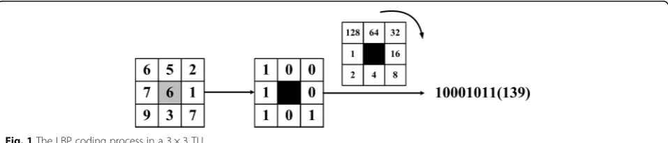
Experiments in [18–20] show that the FLBP and NRLBPs are two representative hand-crafted feature ex-traction methods to face recognition under noise based on LBP. Figure 1 shows the LBP coding process in a 3 × 3 TU.

The definition of the LBP operator of the central gray pixelgcin a 3 × 3 TU is defined as follows:

LBP g_c ¼X8

p¼1S gc¼gp

2p; ð2Þ

s xð Þ ¼ 1;x≥0

1;x<0

; ð3Þ

wheregc is the gray value of central pixel andgpare the

gray values of its neighbors.

2.3.1 FLBP

A drawback of the basic LBP is that a small image vari-ation may alter the LBP code, and thus, it is very sensi-tive to image noise. To tackle this problem, a probability measure is used in fuzzy LBP [18] to represent the

likelihood of a pixel difference to be encoded as “0” or

“1”. SLBP in (4) is the operator of the central gray pixel in the FLBP.

SLBPð Þ ¼i Y

P−1

p¼0

bp ið Þf1;d gc−gp

þ 1−bpð Þi

f0;d gc−gp

h i

;

ð4Þ

f_1;dð Þ ¼Z

0;z ≤ −d

0:5þ0:5z

d;j jZ <d

1;z ≥ d

8 <

: ; ð5Þ

f_0;dð Þ ¼z 1−f_1;dð Þz ; ð6Þ

where bp(i)ϵ{0,1} is the value of the p-th bit of binary

representation of i,d is a thread holding which controls the amount of fuzzification the function performs, andP

is the neighbor number in a TU. Usually, the histogram of FLBP codes is constructed as the feature extracted from an image block and the number of the FLBP histogram bins is 28in a 3 × 3 TU. In the real-world applications, a face image is usually separated intoN> 10 blocks to get a better recognition result.

2.3.2 NRLBPs

NRLBP, NRLBP+, and NRLBP++ are another kind of method to improve the performance of LBP for face rec-ognition under noise. In the NRLBP, the pixel difference

zpbetween the neighboring pixel and the central pixel is

encoded as:

bp¼

1;if zp≥t

X;ifj jZp

0;ifZp≤ −t <t;

8 <

: ð7Þ

whereX ϵ{0,1}is an uncertain state andtis a threshold. An uncertain code C(X) in this state can be expressed as:

C Xð Þ ¼b

⋯

!

;

The NRLBP codes are obtained as (9) based the uncer-tain code:

SNRLBP¼fC Xð ÞjX∈f0;1gn;C Xð Þ∈Φug ð9Þ

whereΦu denotes the collection of all the uniform LBP

[19] codes. According to the definition of the uniform LBP, there are 59 histogram bins of the NRLBP in an image block.

NRLBP+ and NRLBP++ are two improved versions of NRLBP, and the detailed descriptions of them can be found in [19, 20].

3 Noise-resistant network (NR-Network)

Previous researches have shown that deep architectures effectively generate robust features by exploiting the

complex non-linear interactions in the data [46]. Many excellent convolutional neural networks have been pro-posed in recent years and also get some significant results on face recognition. But to the best of our knowledge, there is still no specialized network designed to recognize faces injected with serious noise. In this section, we first present a novel deep convolutional neural network termed NR-Network and then give a description of the training process of our network.

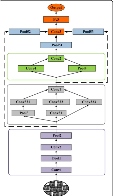
3.1 The network architecture

We used CNN with rectified linear units (ReLUs) [41], max pooling, dropout, and softmax regression. CNNs are feed-forward neural networks designed to deal with large input data, such as those seen in image classification tasks. CNNs are mainly comprised of three types of layers. These are convolutional layers, pooling layers, and fully con-nected layers. When these layers are stacked, a CNN architecture has been formed.

3.1.1 Convolutional layer

The convolutional layer is composed of several convolu-tional kernels which are used to compute different fea-ture maps. The new feafea-ture map can be obtained by first convolving the input with a learned kernel followed by the adoption of an element-wise nonlinear activation function on the convolved results. There are four param-eters to be considered in this layer: the depth, the filter, the stride, and the setting padding. The depth indicates the number of output feature maps. Reducing this param-eter can significantly reduce the total number of neurons of the network, but it can also significantly reduce the pat-tern recognition capabilities of the model.

3.1.2 Pooling layer

The aim of this layer is to gradually reduce the dimen-sion of the representation feature and thus further re-duce the number of parameters and the computational complexity of the model. It is often placed between two convolutional layers or convolutional layer and fully con-nected layer. In our model, the max pooling is used for two reasons: (1) By eliminating non-maximal values, it reduces computation for the upper layers. (2) It provides a form of translation invariance.

3.1.3 Fully connected layer

There may be one or more fully connected layers to per-form high-level reasoning after several convolutional layers and pooling layers. They take all neurons in the previous layer and connect them to every single neuron of current layer to generate global semantic information.

(Fc5). Figure 2 is the overview of the network architecture. During training, the input to our NR-Network is a fixed-size 64 × 64 gray image. The image is passed through a stack of convolutional layers and pooling layers. The output is a 256-cph. Though there are many image compression and High Efficiency Video Coding methods to speedup information transmission [47, 48], a shorter feature size still benefits the real-time face recognition system.

Part 1 labeled purple in Fig. 2 contains two convolu-tional layers, and each layer is followed by a max pooling layer, respectively. Convolutional layer 1 (Conv1) has 5 × 5 filters and a depth of 20. The convolution stride is set to 1 pixel. Following it, max pooling (Pool1) is per-formed over a 3 × 3 pixel window, with stride 2. The convolutional layer 2 (Conv2) has 3 × 3 filters which is the smallest size to capture the information of left to

right, top to bottom, center. The depth of this convolu-tional layer is fixed to 20. Pool2 is also a max pooling layer with a 2 × 2 pixel window to further down sample the outputs of Conv2. We used ReLUs as an activation function for each neuron in the convolutional layers. ReLU is one of the most used activation functions. The definition of the ReLU activation functions is shown as:

a¼ maxðz;0Þ ð10Þ

where z and a are the input and output of activation function, respectively. Experiments in [41] show that deep convolutional neural networks with ReLUs train several times faster than their equivalents withtanhunits.

Next, part 2 marked in gray is an inception module which contains one max pooling layer and four convolu-tional layers with different kernel sizes. Inception mod-ule is introduced by Szegedy et al. [25], which can be seen as a logical culmination of network in network (NIN). They use variable filter sizes to capture different visual patterns of different sizes and approximate the op-timal sparse structures by the inception module. Pool3 in the first line of this inception is a max pooling layer with a 3 × 3 pixel window; the stride of Pool3 is set to be 2 pixels. Convolutional layer 31 (Conv31) has 3 × 3 filters, with stride 1. The upper line of this inception contains three convolutional layers (Conv321, Conv322, and Con323) with different kernel sizes, and strides of these convolution layers are all fixed to 1. Specifically, in one of the configuration, we use the 1 × 1 convolutional filter which can be seen as a linear transformation of the input of the lower layer. Finally, the outputs of the three convo-lutional layers are connected together by a concat layer (Conc1).

After this inception module, part 3 marked in green in Fig. 2 with a max pooling layer and a convolutional layer is inserted. Convolutional layer 4 (Conv4) has 3 × 3 fil-ters, and the depth is 40. The filter size of the max pooling layer (Pool4) in this inception is set to be 2 × 2 to have a same output size with Conv4. Following the inception is also a concat layer (Conc2) as part 2.

In order to extract both the low-level and high-level features hierarchically, the final fully connected layer is connected to the outputs of all the three parts with 256 hidden neurons. The output of this fully connected layer serves as the face representation. Followed by the final inner product layer are the normalization and dropout. Normalization ensures that the derived relative distance of two images has an upper bound, while the objective of the dropout is to reduce the risk of network overfit-ting, which is first introduced by Hinton et al. [46]. The dropout is an effective method to prevent the network to be too dependent on any single neuron and force the network to be more accurate at the same time.

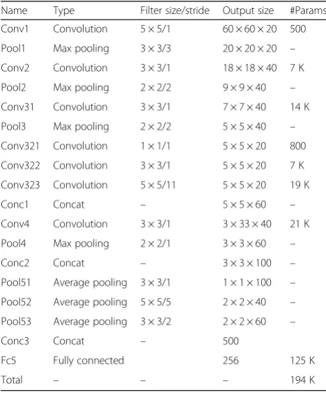
In the proposed network, following the output per part is an average pooling layer marked in blue to adjust the proportions of every part in the final feature. The aver-age pooling layer 51 (Pool51) and averaver-age pooling layer 53 (Pool53) have the same filter size of 3 × 3. The strides of them are set to 1 and 2 pixels, respectively. The aver-age pooling layer 52 (Pool53) has 5 × 5 filters and a stride of 5 pixels. Table 1 describes the specific configur-ation of this NR-Network. The fourth column of Table 1 indicates the outputs of every functional sections of the network. It is clear that the total neurons of part 1, part 2, and part 3 are 160 (2 × 2× 40), 240 (2 × 2 × 60), and 100, respectively. The part 1 indicates the lowest de-scription of the face, and it can provide a global facial contour feature after the pooling of Pool52. In contrast, the output of part 3 is the highest-level face feature ex-tracted from the input face which represents the crucial detailed information of a face and is also very sensitive to noise at the same time. The role of part 2 is to get a balance between different levels of the feature. These multi-level features are combined together to get a more robust face feature.

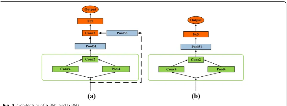
Figure 3(a) and (b) are two benchmark networks named as BN1 and BN2, which are discussed in the fol-lowing sections. For simplicity, we just show several top layers of BN1 and BN2 in Fig. 3 and the rest layers in-cluding the depth, filter size, and stride are same with the proposed NR-Network in Fig. 2. Compared with the

NR-Network, the final fully connected layer (Fc5) of BN1 is connected with the outputs of part 2 and part 3. However, in BN2, only the output of part 3 is connected to the fully connected layer (Fc5). We also use ReLUs in all the convolutional layers of BN1 and BN2 to avoid the vanishing gradient problem. Besides, batch normaliza-tions (BN) are also used for all convolutional layers to be less careful about initialization. BN is an efficient method proposed by Ioffe et al. [49] in 2015. When the data flow through a deep network, the distribution of the input data to the internal layers may be changed; thus, the network will lose the learning capacity and ac-curacy. BN fixes the mean and variances of the input layers to solve this so-called problem which can be seen as a normalization step.

3.2 Training methodology

There are two steps in the training process: forward propagation and back propagation. The aim of the for-ward propagation is to compute the actual classification results of the input data with current parameters. The back propagation is employed to update the parameters during the training process with the objective of making the difference between the actual classification output and the desired classification output as small as possible. To obtain a noise-resistant model, the proposed net-work is trained by the CASIA-WebFace dataset [50]. The CASIA-WebFace dataset is collected from the web-site including 10,575 subjects with 494,414 face images. The size of this dataset ranks second in the literature, only smaller than the private dataset of Facebook. For each subject, there exist several false images with wrong identity labels and few duplicate images. In order to get a balance between different subjects, we remove the sub-jects having less than 14 and more than 200 face images from the dataset. The cleaned CASIA-WebFace dataset used in our network finally contains 8792 subjects with 402,852 face images.

In the training stage, first, all the face images of the CASIA-WebFace are converted to gray scale and nor-malized to 64 × 64. After the normalization, the only preprocessing we do is subtracting the mean gray value which is computed on the training set from each pixel. Before being input to the network, we then inject the Gaussian noise, the uniform noise, and the salt and pepper noise of various noise levels onto the images as Section 4. This is critical to train a noise robust network. The images are split in ratios of 90 and 10% for training and testing, respectively, where 360,000+ images are used to train the network and the remaining 40,000+ are used for testing. The network is implemented by Caffe toolbox [51]. Stochastic Gradient Decent (SGD) is used for optimization in our model with back propagation. We set the weight decay and momentum to 0.005 and

Table 1The specific configuration of the NR-Network

Name Type Filter size/stride Output size #Params

Conv1 Convolution 5 × 5/1 60 × 60 × 20 500

Pool1 Max pooling 3 × 3/3 20 × 20 × 20 –

Conv2 Convolution 3 × 3/1 18 × 18 × 40 7 K

Pool2 Max pooling 2 × 2/2 9 × 9 × 40 –

Conv31 Convolution 3 × 3/1 7 × 7 × 40 14 K

Pool3 Max pooling 2 × 2/2 5 × 5 × 40 –

Conv321 Convolution 1 × 1/1 5 × 5 × 20 800

Conv322 Convolution 3 × 3/1 5 × 5 × 20 7 K

Conv323 Convolution 5 × 5/11 5 × 5 × 20 19 K

Conc1 Concat – 5 × 5 × 60 –

Conv4 Convolution 3 × 3/1 3 × 33 × 40 21 K

Pool4 Max pooling 2 × 2/1 3 × 3 × 60 –

Conc2 Concat – 3 × 3 × 100 –

Pool51 Average pooling 3 × 3/1 1 × 1 × 100 –

Pool52 Average pooling 5 × 5/5 2 × 2 × 40 –

Pool53 Average pooling 3 × 3/2 2 × 2 × 60 –

Conc3 Concat – 500

Fc5 Fully connected 256 125 K

0.9, respectively. The base learning rate is initially set to 0.01 which will decreases through iterations. For the sake of fairness, in our experiments, the training methodologies of the NR-Network and the two benchmark networks BN1 and BN2 are the same.

It is clear that the proposed network can extract a 256 dimensional feature from an input face image. Compared with the feature size of FLBP and NRLBPs given in Section 2, the feature size of NR-Network is much shorter and hence benefits the real-time application.

4 Experimental results and discussions

We compare the proposed network with BN1, BN2, FLBP, and NRLBPs on the AR database injected with Gaussian noise, uniform noise, and salt and pepper noise. For FLBP and NRLBPs, all the images are normalized to 100 × 80 pixels and divided into 20 patches of 20 × 20 pixels. For the NR-Network, BN1, and BN2, the images are normal-ized to 64 × 64 pixels.

4.1 The database and implementation details 4.1.1 AR database

The AR database is of high image quality and considered as a face database having almost no image noise. In this paper, a subset that contains 100 subjects is chosen from the AR database. Fourteen images with only facial expres-sions and illumination changes were taken per subject for our experiments.

The performances of different methods are evaluated by the recognition rate. In the experiments, 14 runs are performed in order to obtain the average recognition rate. In each run, only one image per subject is selected as the gallery set in turn, and the rest 13 images as the probe set. Finally, the 14 recognition rates are averaged as the final result.

In the classification process, the similarity between extracted features of the gallery set and the probe set is

evaluated by the nearest-neighbor classifier with different distance measures. For FLBP and NRLBPs, Chi-square distance (CS), histogram intersection (HI), and modified G-statistic (MG) are utilized in our experiments, which are defined in Eq. (11), Eq. (12), and Eq. (13), respectively. But experimental results show that CS, HI, and MG are not suitable for the NR-Network, BN1, and BN2. There-fore, in the following experiments, the Pearson correlation coefficient, Euclidean distance, and Cosine distance are used to measure the similarity for the networks BN1, BN2, and NR-Network. Table 2 shows some of the recognition rates of the networks using different distance measures on the AR database injected with Gaussian noise (σ= 0.05).

X2ðx;yÞ ¼X

i;j

xi;j−yi;j

2

xi;jþyi;j

ð11Þ

DHIðx;yÞ ¼− X

i;jmin xi;j;yi;j

ð12Þ

DMGðx;yÞ ¼− X

i;jxi;jlog xi;jþyi;j

ð13Þ

where x, y are the concatenated feature vectors and xi,j

andyi,jare thejthdimension of theithpatch, respectively.

We set 0 log(0) = 0, whenxi,j=yi,j= 0. Fig. 3Architecture ofaBN1 andbBN2

Table 2The average recognition rates of the networks using different distance measures on the AR database

BN2 BN1 NR-Network

Chi-square distance 0.8079 0.8187 0.8212

Histogram Intersection 0.8138 0.8243 0.8314

Modified G-statistics 0.8147 0.8207 0.8224

Pearson Correlation Coefficient 0.8234 0.8368 0.8514

Euclidean Distance 0.8157 0.8350 0.8509

The Pearson correlation coefficient, the Cosine dis-tance, and the Euclidean distance are formulated as Eq. (14), Eq. (15), and Eq. (16).

rðx;yÞ ¼ n

X ixiyi−

X ixi

X iyi ffiffiffiffiffiffiffiffiffiffiffiffiffiffiffiffiffiffiffiffiffiffiffiffiffiffiffiffiffiffiffiffiffiffiffiffiffiffi

nX

ix

2

i−

X ixi

2

r ffiffiffiffiffiffiffiffiffiffiffiffiffiffiffiffiffiffiffiffiffiffiffiffiffiffiffiffiffiffiffiffiffiffiffiffiffiffi

nX

iy

2

i−

X iyi

2

r

ð14Þ

Dcðx;yÞ ¼

X ixiyi ffiffiffiffiffiffiffiffiffiffiffiffi X

ix

2

i

q ffiffiffiffiffiffiffiffiffiffiffiffiX iy

2

i

q ð15Þ

DEðx;yÞ ¼ X

iðxi−yiÞ ð16Þ

wherex,yare the feature vectors extracted from the net-works andxiandyiare thei

th

dimension of the vector. The experiments in this paper are conducted on an Intel Xeon E5 2.4GHZ machine with 32G RAM.

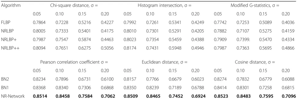
4.2 Face recognition on the AR database with noise FLBP and NRLBPs have been demonstrated effectively for face recognition under noise [18–20], and we have also given some detailed descriptions of them in Section 2. Thus, the proposed network is compared with FLBP and NRLBPs to evaluate the noise-resistant property. Be-sides, we also compare the NR-Network with benchmark networks to testify the effectiveness of the “multi-input” structure. The AR database is injected with Gaussian noise, uniform noise, and salt and pepper noise of four different noise levels referring to [19, 20]. The experimen-tal results on recognition rates are presented in Tables 3, 4, and 5. For the results obtained using the proposed NR-Network, see row 7 in the tables and the results are marked in bold. For the results obtained using the BN1 and BN2, see row 6 and row 5, respectively.

Resistant to Gaussian noise: Normalize the images in range of (0, 1) and then apply Gaussian noise with zero mean and standard derivation of σ. In

Table 3The average recognition rates of different methods on the AR database injected with Gaussian noise

Algorithm Chi-square distance,σ= Histogram intersection,σ= Modified G-statistics,σ=

0.05 0.10 0.15 0.20 0.05 0.10 0.15 0.20 0.05 0.10 0.15 0.20

FLBP 0.7864 0.7228 0.5216 0.4227 0.7992 0.7261 0.5341 0.4249 0.7742 0.7253 0.5089 0.4036

NRLBP 0.8005 0.7333 0.5401 0.4175 0.8010 0.7301 0.5291 0.4205 0.7882 0.7107 0.5275 0.4159

NRLBP+ 0.7987 0.7547 0.5874 0.4463 0.8023 0.7354 0.5459 0.4388 0.7909 0.7399. 0.5470 0.4334

NRLBP++ 0.8094 0.7651 0.6275 0.5056 0.8174 0.7431 0.5948 0.4946 0.7987 0.7363 0.5695 0.4866

Pearson correlation coefficientσ= Euclidean distance,σ= Cosine distance,σ=

0.05 0.10 0.15 0.20 0.05 0.10 0.15 0.20 0.05 0.10 0.15 0.20

BN2 0.8234 0.7896 0.6731 0.6100 0.8157 0.7766 0.6679 0.6023 0.8274 0.7832 0.6779 0.6088

BN1 0.8368 0.8340 0.7306 0.6868 0.8350 0.8239 0.7189 0.6788 0.8414 0.8301 0.7258 0.6815

NR-Network 0.8514 0.8458 0.7584 0.7062 0.8509 0.8465 0.7452 0.6924 0.8523 0.8483 0.7595 0.7096

The bold indicates the best

Table 4The average recognition rates of different methods on the AR database injected with uniform noise

Algorithm Chi-square distance, p = Histogram intersection, p = Modified G-statistics, p =

0.10 0.20 0.40 0.70 0.10 0.20 0.40 0.70 0.10 0.20 0.40 0.70

FLBP 0.7932 0.7574 0.6017 0.5055 0.7889 0.7623 0.6080 0.5184 0.7801 0.7562 0.6198 0.4827

NRLBP 0.7999 0.7670 0.6244 0.5159 0.8018 0.7624 0.6205 0.5020 0.7991 0.7571 0.6282 0.4732

NRLBP+ 0.8264 0.7747 0.6804 0.5465 0.8222 0.7843 0.6731 0.5263 0.8201 0.7769 0.6849 0.5233

NRLBP++ 0.8313 0.7945 0.6936 0.5363 0.8226 0.7816 0.6812 0.5295 0.8291 0.7861 0.6889 0.5321

Pearson correlation coefficient, p = Euclidean distance, p= Cosine distance, p =

0.10 0.20 0.40 0.70 0.10 0.20 0.40 0.70 0.10 0.20 0.40 0.70

BN2 0.8489 0.8065 0.7172 0.6438 0.8391 0.8028 0.6990 0.6289 0.8462 0.8109 0.7205 0.6462

BN1 0.8496 0.8375 0.7531 0.6997 0.8478 0.8342 0.7421 0.7025 0.8515 0.8418 0.7565 0.7063

NR-Network 0.8687 0.8463 0.7974 0.7242 0.8643 0.8409 0.7884 0.7165 0.8795 0.8559 0.7985 0.7275

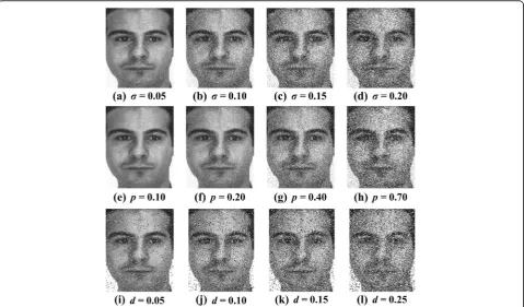
the experiments, σ is set to be 0.05, 0.10, 0.15, and 0.20. The first row of Fig. 4 shows some samples of the noisy images. The average recognition rates on the AR database injected with Gaussian noise are given in Table 3 which shows the proposed NR-Network significantly outperforms the FLBP and NRLBPs regardless of the distance measures. When the images are severely distorted by noise, e.g.,σ= 0.20, the NR-Network

can also achieve acceptable recognition rates of 0.7062 for the Pearson correlation coefficient, 0.6924 for Euclidean distance, and 0.7096 for Cosine distance. However, the recognition rates of the FLBP and NRLBPs are almost lower than 50% in this case.

It is also clear that the performance of the BN1 is bet-ter than BN2. While the NR-Network outperforms both of them under different noise levels using three distance

Table 5The average recognition rates of different methods on the AR database injected with salt & pepper noise

Algorithm Chi-square distance, d = Histogram intersection, d = Modified G-statistics, d =

0.05 0.10 0.15 0.25 0.05 0.10 0.15 0.25 0.05 0.10 0.15 0.25

FLBP 0.6959 0.6236 0.4462 0.2794 0.6908 0.6051 0.4277 0.2669 0.6938 0.6103 0.4451 0.2753

NRLBP 0.7149 0.6743 0.5605 0.3127 0.6995 0.6526 0.5663 0.3075 0.7077 0.6774 0.5742 0.3142

NRLBP+ 0.7344 0.7014 0.6112 0.3943 0.7138 0.6978 0.6041 0.3822 0.7210 0.7059 0.6089 0.4075

NRLBP++ 0.7390 0.7122 0.6242 0.4148 0.7249 0.7088 0.6158 0.4043 0.7365 0.7154 0.6228 0.4297

Pearson correlation coefficient, d = Euclidean distance, d = Cosine distance, d =

0.05 0.10 0.15 0.25 0.05 0.10 0.15 0.25 0.05 0.10 0.15 0.25

BN2 0.8023 0.7615 0.7002 0.5928 0.8144 0.7502 0.6948 0.5965 0.8014 0.7793 0.7046 0.5943

BN1 0.8310 0.8012 0.7534 0.6443 0.8245 0.7993 0.7315 0.6178 0.8327 0.8089 0.7412 0.6332

NR-Network 0.8542 0.8327 0.7886 0.7013 0.8487 0.8214 0.7749 0.6932 0.8597 0.8412 0.7924 0.7107

The bold indicates the best

Fig. 4The sample images of AR database injected with different noise.a–dThefirst lineof Fig. 4 indicates the samples injected with Gaussian noiseσ= 0.05, 0.10, 0.15, 0.20.e–hThesecond lineindicates the samples injected with uniform noisep= 0.10, 0.20, 0.40, 0.70.i–lThethird line

measures. This is because the fully connected layer of the NR-Network has more inputs from the lower layers and hence can extract a multi-level and more discrim-inative feature.

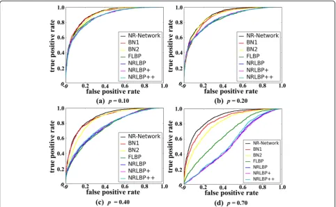
Resistant to uniform noise: Uniform noise is another common type of noise. As the same with adding Gaussian noise, we conduct experiments on the AR database injected with additive uniform noise in the range of (−p/2,p/2). We setp= 0.1, 0.2, 0.4, and 0.7, respectively. Some samples are shown in the second row of Fig.4. It is clear that when the noise level is high, it is barely difficult to recognize a subject by human. Table4summarizes the recognition rates on the AR database with uniform noise. Apparently, the proposed NR-Network is visibly better than the FLBP and NRLBPs and better than BN1 and BN2.

For a higher noise level,p= 0.7, the NR-Network can still obtain achievable results while the FLBP and NRLBPs nearly fail to work.

Resistant to salt and pepper noise: The images in the AR database are also injected with salt and pepper noise to test the performance of different methods. Salt and pepper noise is composed by two noise components: salt noise and pepper noise. Salt noise is the bright spot and pepper noise is the darker spot, which generally appear in the image at the same time. The third row in Fig.4shows some samples injected with salt and pepper noise with different noise densityd= 0.05, 0.10, 0.15, and 0.25. Table5lists the average recognition rates of different methods for face recognition under salt and pepper noise. From the table, we can see that, compared with the Gaussian noise and the uniform

Table 6The feature extraction time (Fea_time) of different methods on the AR database injected with Gaussian noise

FLBP NRLBP NRLBP+ NRLBP++ BN2 BN1 NR-Network

σ= 0.05 Fea_time (s) 0.6806 0.3988 0.7301 0. 7845 0.2694 0.2721 0.2743

σ= 0.10 Fea_time (s) 0.5990 0.2609 0.6365 0.6740 – – –

σ= 0.15 Fea_time (s) 0.5425 0.6832 1.2452 1.3580 – – –

σ= 0.20 Fea_time (s) 0.3553 0.2078 0.6405 0.6973 – – –

noise, the recognition rates of the FLBP and NRLBPs drops much sharply when the images are injected with the salt and pepper noise. Especially, when the noise level is higher thand= 0.15, the recognition rates of the FLBP and NRLBPs are even lover than 40%. However, it is observed from Table5that our proposed method can still give some significant recognition results even when the face images are seriously polluted by this kind of noise.

From the above Tables 3, 4, and 5, we can conclude that the proposed NR-Network cares little about the noise type and distance measures. Beyond that, the per-formance of the NR-Network can still be acceptable in some really bad noise conditions, which indicates that the feature extracted from the “multi-input” structure is more robust to noise. We also compare the feature ex-traction time (Fea_time) per sample of the methods compared in the experiment, and the results are shown in Table 6. We also calculate the classification time of different methods based on the nearest-neighbor classi-fier with Euclidean distance: FLBP with 0.007079 s per sample, NRLBPs with 0.005682 s per sample, and net-works with 0.005043 s per sample. We can see from

Table 6 that the feature extraction time of LBP-based al-gorithms (FLBP and NRLBPs) varies along with the noise level and it is also much higher than the proposed networks. But the feature extraction time of the BN1, BN2 and NR-Network is nearly constant.

Finally, we want to illustrate that the recognition rates of FLBP and NRLBPs established in Tables 3 and 4 are not as good as ref [19] and ref [20]. The reason is prob-ably that there is no preprocessing process during our experiments such as image cropping and rotation. Be-sides, the subset of the AR database used in our experi-ment includes 100 subjects, but the subset used in ref [19] and ref [20] contains only 75 subjects.

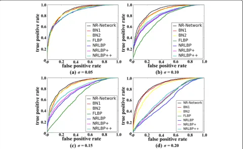
4.3 ROC comparisons

For quantitative evaluation, we also present the ROC (re-ceiver-operating Ccaracteristic) curves of all the algorithms compared in our experiments. The test set from the AR database includes 4050 face pairs, half of which is genuine and the other half is impostor. Figures 5 and 6 show the ROC curves in AR database injected with Gaussian and Uniform noise. The results of images injected with the salt and pepper noise are similar with the Gaussian noise; thus, in this experiment we did not show the ROC curves in this case. We find that the NR-Network can always achieve the

best results on ROC curves in all cases. Besides, the ROC curves of the NR-Network vary slightly along with the noise types and levels. In contrast, the performance of the FLBP, NRLBPs would degrade quickly when the noise level im-proves. According to the results presented in Figs. 5 and 6 for different networks, it is also clear that the NR-Network with multi-input structure is superior to the benchmark networks BN1 and BN2 with fewer inputs to the final fully connected layer which demonstrates the effectiveness of the proposed“multi-input”structure.

4.4 Face recognition under varying illumination

Illumination variation is another challenging task in face recognition. In this section, we conduct an experiment on the CMU-PIE database to further evaluate the per-formance of the proposed “multi-input” structure for face recognition under varying illumination. There are 68 subjects with 41,368 images captured under different illumination, pose, and expression. In this experiment, we choose the illumination subset (21 images per subject) to test the methods, in which one image per subject is chosen as the gallery each turn and the rest 20 images are used as the query. Experimental results show that the LBP-based methods (FLBP, NRLBPs) can get achievable results in glo-bal illumination variation, while the recognition rates of these methods drop sharply under local illumination vari-ation. Thus, in this experiment, we also compare the pro-posed networks with another several state-of-the-arts: Gradient faces (G-face) [52], Weber-Face (W-face) [53], and Local-Gravity-Face (LG-face). Table 7 shows the com-parable recognition rates on the CMU-PIE database.

The similarity between extracted features of the gallery set and the probe set is evaluated by the nearest-neighbor classifier with the Euclidean distance measure. The results of Table 7 demonstrate that the proposed network with the multi-input structure can still get excellent results under varying illumination and is superior to the other methods with the highest averaged recognition rate (93.78%).

5 Conclusions

This paper has shown the performance of the deep learning network to face recognition under noise. A new architecture for noise-robust deep feature representation, named NR-Network, is carefully designed to increase in-ter-personal variations and reduce intra-personal varia-tions at the same time. The main objective of our work is to test the performance of the proposed multi-input structure; thus, the designed NR-Network just consists

of three basic parts for simplicity. The recognition rate with different noise types and ROC results validate that the NR-Network is evidently effective than other well-known noise-resistant face recognition algorithms. With the hierarchical high-level and low-level feature extraction mechanism, the presented network can still work well even at the high noise level based on a single face image. We also analyze the feature size of the ap-proaches compared in our experiments. The final output layer with just 256 hidden neurons of the NR-Network is rather economic. One shall note that we refrain to directly compare our tailored noise-resistant network against other state-of-the-art deep learning models. The main reason is that to the best of our knowledge, there is no specified net-work designed to solve the problem of face recognition af-fected by noise as addressed by our model. One possible future work is to involve sparsity based models [54], match-ing based methods [55], and error-correction based models [56] to further improve cost effectiveness and robustness.

Abbreviations

BN:Batch normalizations; CNN: Convolutional neural networks; CS: Chi-square distance; FLBP: Fuzzy local binary pattern; HI: Histogram intersection; ILSVRC: ImageNet Large-Scale Visual Recognition Challenge; MG: Modified G-statistic; NIN: Network in network; NRLBP: Noise-resistant LBP; NR-Network: Noise-resistant network; ReLUs: Rectified linear units; ROC: Receiver-operating characteristic; SGD: Stochastic gradient decent

Acknowledgements Not applicable.

Funding

This paper is sponsored by the Natural Science Foundation of Shanghai, Fund No. 14ZR1447200.

Availability of data and materials All data are fully available without restriction.

Author_’s contributions

YD implemented the core algorithm and drafted the manuscript. YC and XC conducted the experiments and performed the statistical analysis. BL, XY, and XBY helped to design the experiments. All authors read and approved the final manuscript.

Competing interests

The authors have declared that no competing interests exist.

Consent for publication Not applicable.

Ethics approval and consent to participate Not applicable.

Publisher’s Note

Springer Nature remains neutral with regard to jurisdictional claims in published maps and institutional affiliations.

Table 7The average recognition rates of different methods on the CMU-PIE database for face recognition under varying illumination

Algorithm FLBP NRLBP++ LG-face W-face G-face BN2 BN1 NR-Network

Recognition rate 0.5489 0.5744 0.8863 0.8898 0.9093 0.9122 0.9234 0.9378

Author details

1_{Shanghai Institute of Microsystem and Information Technology, Wireless}

Sensor Network Laboratory, Chinese Academy of Sciences, No. 1455 Pingcheng Road, Jiading District, Shanghai 201800, China.2University of Chinese Academy of Sciences, No. 19A Yuquan Road, Beijing 100049, China.

Received: 1 March 2017 Accepted: 2 June 2017

References

1. Padmapriya S, Kalajames E A, Real Time Smart Car Lock Security System Using Face Detection and Recognition. In Proceedings of the IEEE Conference on Computer Vision and Pattern Recognition (CVPR), 2012, pp. 1–6 2. Z Xu, C Hu, L Mei, Video structured description technology based

intelligence analysis of surveillance videos for public security applications. Multimed. Tools Appl.75(19), 1–18 (2015)

3. Z Xu, Y Liu, H Zhang et al., Building the multi-modal storytelling of urban emergency events based on crowdsensing of social media analytics. Mob. Netw. Appl.22(2), 218–227 (2017)

4. Y Yang, Z Xu et al., A security carving approach for AVI video based on frame size and index. Multimedia Tools Appl.76(3), 3293–3312 (2017) 5. D Mcallister, Law Enforcement Turns to Face-Recognition Technology.

Information Today.24(5) (2007)

6. Z Yan, Z Xu, JD., The Big Data Analysis on the Camera-based Face Image in Surveillance Cameras. Intell. Autom. Soft Comput.. doi: 10.1080/10798587. 2016.1267251 (2016)

7. Z Xu, et al., The big data analytics and applications of the surveillance system using video structured description technology. Clust. Comput.19(3), 1283–1292 (2016)

8. B Kamgarparsi, W Lawson, B Kamgarparsi, Toward development of a face recognition system for watchlist surveillance. IEEE Trans. Pattern Anal. Mach. Intell.33(10), 1925–1937 (2011)

9. SJ Mckenna, S Gong, Non-intrusive person authentication for access control by visual tracking and face recognition. Lect. Notes Comput. Sci. 1206, 177–183 (2006)

10. H Roy, D Bhattacharjee, Local-gravity-face (LG-face) for illumination-invariant and heterogeneous face recognition. Info. Forensics Secur. IEEE Trans.11(7), 1_–1 (2016)

11. X Wang, Q Ruan, Jin, et al., Three-dimensional face recognition under expression variation. EURASIP J. Image Video Process.54(1): 1–11 (2014) 12. MH Siddiqi et al., Human facial expression recognition using curvelet

feature extraction and normalized mutual information feature selection. Multimedia Tools Appl.75(2), 935–959 (2016)

13. J Xu, K Zhang, M Xu, Z Zhou, An adaptive threshold method for image denoising based on wavelet domain. Proc. SPIE Int. Soc. Opt. Eng.7495, 165 (2009)

14. J Portilla, V Strela et al., Image denoising using scale mixtures of Gaussians in the wavelet domain. IEEE Trans. Image Process.12(11), 1338–1351 (2003) 15. F Luisier, T Blu, M Unser, A new SURE approach to image denoising:

interscale orthonormal wavelet thresholding. IEEE Trans. Image Process. 16(3), 593–606 (2007)

16. BA Olshausen, DJ Field, Sparse coding with an overcomplete basis set: a strategy employed by V1? Vision Res.37(23), 3311–3325 (1997)

17. M Elad, M Aharon, Image denoising via sparse and redundant representations over learned dictionaries. IEEE Trans. Image Process.15(12), 3736–3745 (2006) 18. T Ahonen, M Pietikainen, Soft histograms for local binary patterns. Proc.

FINSIG2007, 1–4 (2007)

19. J Ren, X Jiang, J Yuan, Noise-resistant local binary pattern with an embedded error-correction mechanism. IEEE Trans. Image Process.22(10), 4049–4060 (2013) 20. J Ren, X Jiang, J Yuan, LBP Encoding, Schemes jointly utilizing the

information of current bit and other LBP bits. IEEE Signal Process Lett. 22(12), 2373_–2377 (2015)

21. GB Huang, M Ramesh, T Berg, E Learned-Miller, Labeled faces in the wild: a database for studying face recognition in unconstrained environments, in

Technical Report 0749(University of Massachusetts, Amherst, 2007) 22. Y Sun, X Wang, X Tang, Deep learning face representation by joint

identification-verification, inConference and Workshop on Neural Information Processing Systems (NIPS), 2014

23. Y Sun, X Wang, X Tang, Deeply learned face representations are sparse, selective, and robust, inProceedings of the IEEE Conference on Computer Vision and Pattern Recognition (CVPR), 2015, pp. 2892–2900

24. K. Simonyan, A. Zisserman, Very deep convolutional networks for large-scale image recognition. CoRR, abs/1409.1556, 2014

25. C Szegedy, W Liu, Y Jia, P Sermanet, S Reed, D Anguelov, D Erhan, V Vanhoucke, A Rabinovich, Going deeper with convolutions, inProceedings of the IEEE Conference on Computer Vision and Pattern Recognition (CVPR), 2015, pp. 1_–9 26. Y Sun, X Wang, X Tang, Sparsifying neural network connections for face

recognition, inProceedings of the IEEE Conference on Computer Vision and Pattern Recognition (CVPR), 2016, pp. 4856_–4864

27. Y Wen, Z Li et al., Latent factor guided convolutional neural networks for age-invariant face recognition, inProceedings of the IEEE Conference on Computer Vision and Pattern Recognition (CVPR), 2016, pp. 4893–4901 28. J Xie, L Xu, E Chen, Image denoising and inpainting with deep neural

networks, inIn Proceedings of the International Conference on Neural Information Processing Systems (NIPS), 2012, 2012, pp. 341–349 29. S Harmeling, Image denoising: can plain neural networks compete with

BM3D? inProceedings of the IEEE Conference on Computer Vision and Pattern Recognition (CVPR), 2012, pp. 2392–2399

30. J Krause, B Sapp, A Howard, H Zhou, A Toshev, T Duerig et al., The unreasonable effectiveness of noisy data for fine-grained recognition, in

European Conference on Computer Vision (ECCV), 2016

31. S Levine, P Pastor, A Krizhevsky, D Quillen, Learning hand-eye coordination for robotic grasping with deep learning and large-scale data collection, in

Proceedings of the International Symposium on Experimental Robotics (ISER), 2016 32. H Xu, J Yan, N Persson, W Lin, H Zha,Fractal dimension invariant filtering and

its CNN-based implementation, 2016. arXiv:1603.06036

33. Y Sun, X Wang, X Tang, Deep learning face representation from predicting 10,000 classes, inProceedings of the IEEE Conference on Computer Vision and Pattern Recognition (CVPR), 2014

34. AM Martinez, The AR face database. Cvc Tech. Rep., 24 (2010)

35. BC Zhang, SG Shan, XL Chen, W Gao, Histogram of Gabor phase patterns (HGPP): a novel object representation approach for face recognition. IEEE Trans. Image Process.16(1), 57_–68 (2007)

36. C Liu, Gabor-based kernel PCA with fractional power polynomial models for face recognition. IEEE Trans. Pattern Anal. Mach. Intell.26(5), 572–581 (2004) 37. T Ahonen, A Hadid, M Pietikainen, Face description with local binary

patterns: application to face recognition. IEEE Trans. Pattern Anal. Mach. Intell.28(12), 2037–2041 (2006)

38. bdulrahman, Gabor Wavelet Transform Based Facial Expression Recognition Using PCA and LBP. In: Signal Processing and Communications Applications Confer and Communications Applications, (2014) pp. 2265–2268 39. Y Tong, R Chen, Y Cheng, Facial expression recognition algorithm using

LGC based on horizontal and diagonal prior principle. Optik - Int. J. Light Electron. Opt.125(16), 4186_–4189 (2014)

40. Z Guo, L Zhang, D Zhang, Rotation invariant texture classification using LBP variance (LBPV) with global matching. Pattern. Recogn.43(3), 706–719 (2010) 41. X Wang, TX Han, S Yan, An HOG-LBP human detector with partial occlusion

handling, inthe proceedings of the IEEE International Conference on Computer Vision, 2009, pp. 32–39

42. J Zhang et al., Boosted local structured HOG-LBP for object localization, in

Proceedings of the IEEE Conference on Computer Vision and Pattern Recognition (CVPR), 2011, pp. 1393_–1400

43. C Zhang, J Yan, C Li, X Rui, L Liu, On estimating air pollution from photos using convolutional neural network, inProceedings of the ACM international conference on Multimedia, 2016, pp. 297_–301

44. R Girshick et al., Region-based convolutional networks for accurate object detection and segmentation. IEEE Trans. Pattern Anal. Mach. Intell.38(1), 142–158 (2016)

45. S Hong, T You, S Kwak, B Han, Online Tracking by Learning Discriminative Saliency Map with Convolutional Neural Network. in Proceedings of International Conference on International Conference on Machine Learning (ICML), 2015, pp. 597–606

46. A Krizhevsky, I Sutskever, G Hinton, Imagenet Classification with Deep Convolutional Neural Networks. Conf. Neural Inf. Process. Syst,25(2), 1097–1105 (2012) 47. C Yan, Y Zhang, J Xu et al., A highly parallel framework for HEVC coding

unit partitioning tree decision on many-core processors. IEEE Signal Process Lett.21(5), 573–576 (2014)

48. C Yan, Y Zhang, J Xu et al., Parallel deblocking filter for HEVC on many-core processor. Electron Lett.50(5), 367–368 (2014)

50. D Yi, Z Lei, S Liao, SZ Li,Learning Face Representation from Scratch, arXiv preprint arXiv:1411.7923, 2014

51. Y Jia, E Shelhamer, J Donahue, S Karayev, J Long, R Girshick, S Guadarrama, T Darrell, Caffe: Convolutional architecture for fast feature embedding. in Proceedings of the 22nd ACM International Conference on

Multimedia(ACM),2014, pp. 675_–678

52. T Zhang, YY Tang et al., Face recognition under varying illumination using gradientfaces. IEEE Trans. Image Process.18(11), 2599–2606 (2009) 53. B Wang, W Li, W Yang et al., Illumination normalization based on Weber’s

law with application to face recognition. IEEE Trans. Signal Process Lett. 18(8), 462–465 (2011)

54. J Yan, M Zhu, H Liu, Y Liu, Visual saliency detection via sparsity pursuit. IEEE Signal Process Lett.17(8), 739–742 (2010)

55. J Yan, M Cho, H Zha, X Yang, S Chu, Multi-graph matching via affinity optimization with graduated consistency regularization. IEEE Trans. Pattern Anal. Mach. Intell.38(6), 1228–1242 (2016)