R E S E A R C H
Open Access
A fast source-oriented image clustering
method for digital forensics
Chang-Tsun Li
1,2and Xufeng Lin
1*Abstract
We present in this paper an algorithm that is capable of clustering images taken by an unknown number of unknown digital cameras into groups, such that each contains only images taken by the same source camera. It first extracts a sensor pattern noise (SPN) from each image, which serves as thefingerprintof the camera that has taken the image. The image clustering is performed based on the pairwise correlations between camera fingerprints extracted from images. During this process, each SPN is treated as a random variable and a Markov random field (MRF) approach is employed to iteratively assign a class label to each SPN (i.e., random variable). The clustering process requires no a priori knowledge about the dataset from the user. A concise yet effective cost function is formulated to allow different “neighbors” different voting power in determining the class label of the image in question depending on their similarities. Comparative experiments were carried out on the Dresden image database to demonstrate the advantages of the proposed clustering algorithm.
Keywords: Image clustering, Markov random fields, Digital forensics, Sensor pattern noise, Multimedia forensics
1 Introduction
Nowadays, digital imaging devices, especially mobile phones with built-in cameras, have become an essential part of modern life. They enable us to record every detail of our life anytime and anywhere. Meanwhile, the rise of social media, such as Facebook, Twitter, and Instagram, has fostered and stimulated our interest in sharing pho-tos and videos of life moments over social networks using mobile imaging devices. On the one hand, social media affords us a new way to express friendship, intimacy, and community. But on the other hand, the difficulty of veri-fying the profiles or identities of users on social networks also gives rise to the cyber crime.
A typical circumstance is that a number of images are collected under proper legal procedures from social net-works for forensic analysis, but the devices which have been used to take these images are not available. If those images can be clustered into a number of groups, each including the images acquired by the same camera, the forensic investigators will be able to link the images to particular devices and in a better position to associate
*Correspondence: [email protected]
1School of Computing and Mathematics, Charles Sturt University, Boorooma Street, Wagga Wagga, Australia
Full list of author information is available at the end of the article
different social media accounts belonging to a person of interest. We refer to this task as source-oriented image clustering. This can be particularly useful in a variety of forensic cases, e.g., identifying fake user profiles, find-ing stolen camera devices, or defendfind-ing against Internet defamation. Fortunately, with the advances in multime-dia forensics, we are able to extract “device fingerprints” from images and videos and trace back to their source device. By resorting to device fingerprints extracted from images, source-oriented image clustering can be divided into two main sequential operations: the extraction of device fingerprintfrom images followed by animage clus-tering operation based on the device fingerprints. The main challenges in this scenario are:
• The investigator does not have the cameras that have taken the photos to generate quality reference device fingerprint.
• No prior knowledge about the number and types of the cameras are available.
• Given the sheer number of photos, analyzing each image in its full size is computationally prohibitive.
1.1 The challenges of source-oriented image clustering and related works
There are many factors that affect the performance of the clustering system. One is the accuracy of the finger-prints extracted from images. Various forms of device fingerprints such as sensor pattern noise (SPN) [1–12], camera response function [13], re-sampling artifacts [14], color filter array (CFA) interpolation artifacts [15, 16], JPEG compression [17], and lens aberration [12, 18] have been proposed in recent years. Other device and image attributes such as binary similarity measures, image quality measures, and higher order wavelet statistics have also been adopted for identifying source imaging devices [19–22]. While many methods [13–16] make specific assumptions in their applications, SPN-based methods [1–12] do not require such assumptions to be satisfied and thus have drawn much more atten-tion. Another merit of SPN is that it is unique to each device, which means it is capable of differentiating indi-vidual devices of the same model [1, 3, 5, 11]. These merits make SPN a good candidate for various digital forensic applications.
Another factor is the system’s effectiveness in clustering images based on device fingerprints. The main objective in clustering applications is to group samples into clusters of similar features (e.g., the SPNs). Among a wide variety of methods,k-means [23, 24] and fuzzyc-means [25–27] have been intensively employed in various applications. However, classicalk-means and fuzzyc-means clustering methods rely on the user to provide the number of clus-ters and initial centroids. Moreover, they are sensitive to outliers, and the computational complexities are very high for high-dimensional data, which make them unsuitable for clustering high-dimensional camera fingerprints.
The difficulty of specifying an appropriate cluster num-ber also exists in graph clustering-based methods, such as [28–30]. In [31], the camera fingerprints clustering is for-mulated as a weighted graph clustering problem, where SPNs are considered as the vertices in a graph, while the weight of each edge is represented by the correlation between the SPN pair connected by the edge. Ak-class spectral clustering algorithm [32] is employed to group the vertices into a number of partitions. To determine the optimal cluster number, the same spectral clustering algo-rithm is repeated for different value ofkuntil the smallest size of the resultant clusters equals 1, i.e., one singleton cluster is generated. However, it is easy to form single-ton clusters when some SPNs are severely contaminated by other interferences. So the feasibility of such manner of determining the optimal cluster number is still an issue.
To work without knowing the number of clusters, the agglomerative hierarchical clustering algorithms [33, 34] were adopted to cluster SPNs. Starting with the pair-wise correlation matrix, the algorithms initially consider
each SPN as a cluster and iteratively merge the two most similar clusters according to the average linkage criterion. At each iteration, an overall silhouette coefficient, which measures the cohesion inside clusters and the separation among clusters, is calculated to measure the quality of partition. This process stops when all SPNs have been merged into one cluster and the partition corresponding to the best clustering quality is deemed as the final par-tition. These two algorithms are relatively slow, because their time complexity isO(N2logN), whereNis the num-ber of SPNs. Another limitation, which also exists in other more advanced hierarchical clustering-based algorithms such as CURE [35], ROCK [36], and CHAMELEON [37], is that once an object is assigned to a cluster, it will not be considered again in the ensuing process [38]. In the con-text of SPN clustering, the misclassification at the earlier stage is likely to induce error propagation in the succeed-ing merge and produce large clusters containsucceed-ing SPNs of different cameras.
Since the intrinsic quality of SPNs depends on many complex factors [11, 12, 39, 40], the average correlation between SPNs of one camera may be significantly different from that of other cameras. Therefore, SPN-based image clustering is a typical problem of finding clusters of differ-ent densities. The classical density-based algorithms, such as DBSCAN [41] and DENCLUE [42], are not applica-ble in this scenario, because their density-based definition of core points cannot identify the core points of varying density clusters. To overcome this problem, a shared near-est neighbor (SNN)-based clustering algorithm has been proposed in [43] to find clusters of different sizes and den-sities. However, choosing appropriate parameters for the algorithm is not easy if the data to be clustered is not well understood.
threshold is calculated from a quadratic curve, whose parameters are obtained by fitting the correlation values of four Canon cameras. However, the threshold’s quadratic dependence on the number of SPNs is questionable. A clustering algorithm requires no a priori knowledge about the nature of the SPNs and the threshold is certainly more desirable.
To overcome the infeasibility of the manner of deter-mining the optimal cluster number in [31], Amerini et al. [45] proposed a blind SPN clustering algorithm based on normalized cut criterion [46]. Similar to [31], SPNs are considered as the vertices in a graph and the weight of each edge measures the similarity between the two vertices connected by the edge. With the pairwise similar-ities between SPNs, the graph is bipartitioned recursively by finding the splitting point that minimizes the corre-sponding normalized cut. This recursive bipartition ter-minates when the mean value of intra-cluster weights is less than a pre-defined threshold Th for all clusters. Th is experimentally set to the value giving the best aver-age performance on five datasets in terms of ROC curves. This normalized cut-based algorithm is fast and was reported to have better performance than [31] and [33] on datasets composed of hundreds of images taken by a few cameras.
More recently, Marra et al. introduced a two-step clus-tering algorithm in [47]. In the first step, the pairwise correlation matrix of SPNs is adjusted by subtracting a constant α = μ0 + 3σ0, where μ0 and σ0 are the mean and standard deviation, respectively, of the inter-camera correlations obtained from a training set. Then, the adjusted correlation matrix is fed into the correla-tion clustering algorithm [48] to generate a large num-ber of over-partitioned clusters. While in the second step, an ad hoc refinement procedure is performed to progressively merge the clusters generated in the first step. The refinement step separates the clusters into two sets, a set of “large” clusters and a set of “small” clus-ters. If the majority of the SPNs in a small cluster are similar to (i.e., by comparing to a pre-defined thresh-old β) the centroid of a large cluster, the small cluster will be merged into the large cluster and the centroid will be updated accordingly. This process continues until no further merge can be performed. This algorithm was reported to outperform almost uniformly the state-of-the-art algorithms [47], but it requires all the SPNs to be retained in the RAM for efficiently updating the cen-troids of clusters, which makes it unsuitable for relatively large datasets.
We presented our preliminary study in [49], where each SPN is treated as a random variable and Markov ran-dom field (MRF) is used to iteratively update the class labels. Based on the pairwise correlation matrix, a refer-ence similarity is determined using thek-means (k = 2)
clustering algorithm and amembership committee, which consists of the most similar SPNs of each SPN, is estab-lished. The similarity values and the class labels assigned to the members of membership committee are used to estimate the likelihood probability of assigning each class label to the corresponding SPN. Then, the class label with the highest probability is assigned to the SPN. This process terminates when there are no more class label changes in two consecutive iterations. This algorithm performs well on small datasets, but its performance dete-riorates as the size of dataset grows. Moreover, it is very slow because the likelihood probability involves all the class labels in the membership committee and has to be calculated for every SPN in every iteration. The time complexity is nearly O(N3) in the first iteration, which makes it computationally prohibitive for large datasets. Therefore, a faster and more reliable algorithm that can handle large datasets is desirable for source-oriented image clustering.
1.2 Our contributions
In view of the aforementioned challenges in the context of device fingerprint-based image clustering, we conduct an in-depth study based on the work in [49] and propose a fast clustering framework for images of unknown sources. It makes several major contributions:
• First, we propose a fast and reliable algorithm for clustering camera fingerprints. Aiming at overcoming the limitations of the work in [49], the proposed algorithm makes the following improvements: (1) redefining the similarity in terms of the shared nearest neighbors; (2) speeding up the calculation of the reference similarity; (3) refining the
determination of the membership committee; (4) reducing the complexity of calculations in each iteration; and (5) accelerating the speed of convergence. Not only the presentation of the clustering methodology is more comprehensive and detailed in this work, but also the proposed algorithm is much more efficient and reliable than that in [49]. • Secondly, we discuss in detail the related SPN
clustering algorithms, namely the spectral, the hierarchical, the shared nearest neighbor, the normalized cut, and our previous MRF-based clustering methods [49]. These algorithms are evaluated and compared on real-world databases to provide insight into the pros and cons of each algorithm and offer a valuable reference for practical applications.
includes only six cameras. Furthermore, the quality of clustering is characterized by F1-measure and Adjusted Rand Index, which are more suitable for evaluating clustering results than only the true positive rate or accuracy used in [31, 33, 34, 49].
1.3 Outline of this paper
The remainder of this work is organized as follows. The formulation and discussion of the proposed algorithm are given in Section 2. In Section 3, respectively. The param-eter selection of the proposed algorithm as well as the comparison with other related works is presented. Finally, Section 5 concludes this work.
2 Methods
To facilitate the clustering, the SPN of a small block at the center of each of the given N images are extracted. AnN×Ncorrelation matrix is established, with one ele-ment,(i,j), representing the correlation between the SPNs of image i and j. Then, an alternative similarity matrix in terms of shared nearest neighbors is constructed from the correlation matrix. By making the pairwise similarities available in the matrix, the system does not have to repeat the similarity calculation when the similarity of the same pair of images is required again in the iterative clustering process. Although the number of image classes (cameras) can be much greater than 2, for each image, there are only two types of similarity: intra-class and inter-class. Based on the similarity matrix, each SPN is treated as a random variable to be assigned a class label, and a refer-ence similarityris estimated to serve as a rough boundary between the intra- and inter-class similarities in order to encode a cost function using a Markov random field (MRF). Separating the similarities into intra- and inter-class similarities enables us to find clusters of different densities, because the average intra-class similarity indi-cates the “density” of the cluster that each SPN belongs to. In the following subsections, we will provide the details of the proposed algorithm.
2.1 SPN extraction
Given an imageI, the following equation is used to extract the SPN,n, from a block of the size specified by the user from the center:
n=I−F(I), (1)
where F is the denoising algorithm proposed in [50]. Each SPN is further preprocessed by the Wiener fil-tering (WF) in the DFT domain [2] to suppress the non-unique artifacts. Note that the reason we do not use our recent preprocessing scheme in [11] is that, the peaks in the DFT spectrum of a single SPN are not as distinct as those in the spectrum of a clean reference SPN.
2.2 Establishment of similarity matrix
During the process of clustering, similarities between SPNs are to be used to determine the class membership of each image (or SPN). As will be seen in Section 2.3.4, the process of class label update, which involves the calculation of similarities between SPNs, has to be iter-ated until the stop criterion is met. However, repeat-ing the similarity calculation of the same SPN pairs is time-consuming. Therefore, the purpose of establishing an N ×N similarity matrix is to calculate the similar-ity only once for each SPN pair. When a similarsimilar-ity value is needed at any stage, the value is retrieved from the similarity matrix. The similarity between any two SPNs ni and nj is initially measured by the normalized cross correlation (NCC)
ρij= (ni− ¯
ni)·(nj− ¯nj)
ni− ¯ni · nj− ¯nj
, i,j∈[ 1,N] , (2)
where · is theL2norm and the mean value is denoted with a bar. In this way, we establish anN × N correla-tion matrix ρ, with elementρij indicating the closeness between SPNs ni and nj. Because of the symmetrical nature of the correlation matrix and that the elements (self-correlations) along the diagonal axis is always 1, only N×(N−1)/2 correlations need to be calculated.
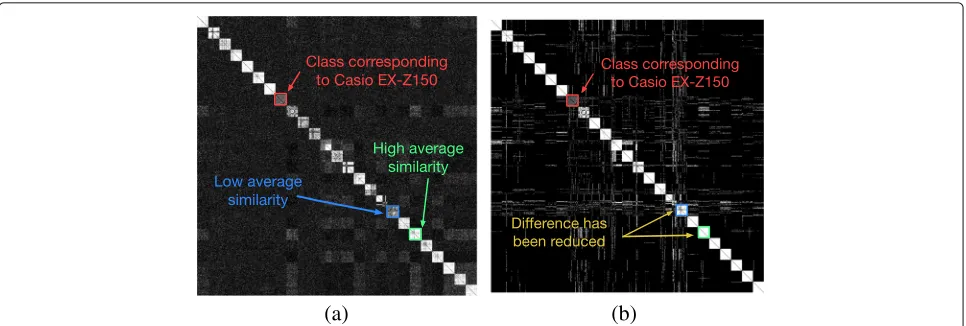
However, due to the varying qualities of SPNs of dif-ferent cameras, the average correlation between SPNs of one camera may be different from that of another cam-era. As exemplified in Fig. 1a, the average correlation the class highlighted by the green rectangle is higher than that of the class highlighted by the blue rectangle. This problem makes the clustering of SPNs more challeng-ing. An alternative definition of similarity in terms of shared nearest neighbors, as proposed in [36, 43, 51], is a promising way to overcome this problem. Specifi-cally, the similarity Wij between two SPNs ni and nj is redefined as
Wij= |N(ni)∩N(nj)|, (3)
(a)
(b)
Fig. 1Pairwise similarities of 1000 images taken by 25 cameras (each responsible for 40 images).aCorrelation matrixρ.bSimilarity matrixWin terms of sharedκ-nearest neighbor (κ=15)
Procedure 1f =fastClustering(W,m)
1: f ←randPerm(N);Assign unique random class labels
2: ri←fastSplit(Wi:,ini,low,high); Find the reference
similarity ofni
3: Ci←establishMC(Wi:,m); Establish the MC ofni
4: pi←0;qi←2;stable←2;iteration←0;
5: whilestable>0or++iteration≤50do
6: fori=1 toNdo
7: ifpithen continue; Stop updating forniif pi=1
8: Li← {fj|j∈Ci}; Class labels in the MC ofni
9: for eachl∈Lido
10: Ui(l,WCi,Li)←
j∈Cis(l,fj)(Wij−ri);
11: end for
12: fˆi←arg minl∈LiU(l,WCi,Li);
13: iffi= ˆfithen
14: fi← ˆfi;pi←0; Update the class label ofni
15: else
16: if--qi<1then
17: pi←1; Stop updating forni
18: end if
19: end if
20: ifipi==0then
21: stable--;
22: end if
23: end for
24: end while
25: returnf;
2.3 Clustering
Taking the similarity matrixW as input, the task of this step is to identify image groups such that each group cor-responds to one camera. Our previous experience of using Markov random field (MRF) approach to image segmen-tation [53, 54] and many others’ successful applications of MRF [9, 55–57] suggest that the local characteristics of MRFs (also known asMarkovianity) allow global opti-mization problems to be solved iteratively by taking local information into account. Suppose there areKclasses of images in the subset, with the value ofK unknown, and denoteD= {dk|k = 1, 2,. . .,K}as the set of class labels andfi ∈Das the class label of SPNni. By considering the labelfi of each SPNni as a random variable, the objec-tive of clustering is to assign an optimal class labeldk to each random variableni in an iterative manner until the stop criterion is met. The pseudo code of clustering is shown in Procedure 1, and the details will be explained as follows.
2.3.1 Assign unique initial class labels
2.3.2 Calculate reference similarity
Although the actual number of classes,K, is unknown, we can expect that normally the similarities between SPNs of the same class (calledintra-class similarity) are greater than the similarities between SPNs of different classes (calledinter-class similarity). So for each SPNni, its inter-class and intra-inter-class similarities are expected to be sepa-rable. In [49], a simplek-means clustering method (k=2) is used to cluster the N −1 similarity values into two groups (one asintra-classand the otherinter-class). Then, the average of the centroids of the two clusters is taken as a reference similarity r to separate the two distribu-tions. However, the general-purposek-means is slow and quickly becomes inefficient for large datasets. Be aware that we are dealing with the binary separation of one-dimensional data, and we have the prior knowledge of the approximate range where the cutoff point should lie in, so we propose a fast method, which shares the same essence as k-means, to iteratively search for the appro-priate cutoff point, as shown in step 2 of Procedure 1, where Wi: is the similarities between ni and the other
(N−1)SPNs.
The details of the algorithm are given in Procedure 2. We assume that the reference similarity r to be deter-mined lies in between [low,high], so the sum and size of the similarities between (0,low) and(high,N) can be pre-calculated before the iterative update. The purposes of limiting the search range to [low,high] are twofold. First, it narrows down the search range and therefore speeds up the search process. Second, it forces the opti-malrto fall within an appropriate range so as to alleviate the problem of “local minimal”. The search process is fur-ther sped up by specifying a valueinias the initial r. In step 6 of Procedure 2,I represents the “binary” (0 or 1) class labels of the similarities in [low,high]. The midpoint of the means of the two classes is used to update r, as provided in step 9 of Procedure 2. The update terminates when label assignments no longer change. Incorporating ini,lowandhighto facilitate the determination ofrmakes the search process faster and more flexible. In some cases, such prior information is already known to the user. In our experiments, low, ini and high were set to 0, 1 and 5, respectively.
The output r of Procedure 2 serves the purpose of dividing the intra- and inter-class similarities and can be used to encode the cost function to be defined in Eq. (6). Although the similarities are both scene- and device-dependent, we could expect that most intra-class similar-ities are greater thanrwhile most inter-class similarities are less thanr. It is also intuitive that, for most cases, a similarity value farther away fromron the left-hand side indicates a higher probability that the two corresponding images are taken by different devices. On the other hand, we have higher confidence in believing that a similarity
value farther away from r on the right-hand side indi-cates that the two corresponding images are taken by the same device. The closer tor, the less confidence we have on the similarity value in telling us the situation. This suggests that, if we treat classification as an optimization problem, the distance between a similarityWijandrcan be used to encode an objective function for guiding the search for the optimal class label of each image. We will explain how we make use of this useful information in Section 2.3.4.
Procedure 2r=fastSplit(v,ini,low,high)
1: L= {vi|vi<low};
2: H= {vi|vi>high};
3: M= {vi|vi≥low&&vi≤high};
4: sz_L←size(L);sum_L←sum(L);
5: sz_H←size(H);sum_H←sum(H);
6: I← {M>ini};
7: do
8: J ←I;
9: r←0.5×sum_L+sum(MI˜)
sz_L+sum(I˜) +
sum_H+sum(MI)
sz_H+sum(I)
;
10: I← {M>r};
11: whileI=J
12: returnr;
2.3.3 Establish membership committee
2.3.4 Update class labels using MRF
During the clustering process, each SPN is iteratively visited and re-labeled until the stop criterion is met. In terms of Markov random fields, when an SPN ni is being visited, the probability p(·) of assigning each class label l currently assigned to the members of Ci is calculated using
p(fi=l|WCi,Li)= 1 Zi
e−Ui(l,WCi,Li), (4)
wherefiis the class label of SPNni,WCiis the similarities between SPNni and the corresponding members ofCi, i.e.,WCi = {Wij|j ∈ Ci}, andLi is the set of class labels currently assigned to the members ofCi, i.e.,Li = {fj|j∈
Ci},l∈Li.Ziis the partition function [25]
Zi=
l∈Li
e−Ui(l,WCi,Li), (5)
where Ui(l,WCi,Li) is the cost of assigning labell to ni givenWCiandLi. It is defined as
Ui(l,WCi,Li)=
j∈Ci
s(l,fj)(Wij−ri), (6)
where Wij is the similarity (see Eq. (2)) between ni and
nj (j ∈ Ci), ri is the reference similarity described in Section 2.3.2, ands(l,fj)is a sign function defined as
s(l,fj)=
+1, l=fj
−1, l=fj. (7)
It is clear to see that the probability of each labellto be assigned tofi is based on the observed data and the cur-rent local class configurationLi. From the cost function
U(·) in Eq. (6), we can see that the closer the similarity Wij is to ri, the less significant nj is in determining the class label for SPNni. From the sign function in Eq. (7) and its role in Eq. (6), we can see that the formulation of Eq. (6) encourages appropriate label assignment with a reward (i.e., anegativecostU(·)to increase the probability of that label). By the same token, it penalizes inappro-priate decisions to reduce the probability of assigning an inappropriate label by imposing apositive costU(·). The following explains these two cases, each with two different scenarios.
• Rewarding appropriate label assignments Scenario 1: IfWij<ri(i.e., SPNsniandnjbelong to different classes) and the label l under investigation is different fromfj(i.e.,l=fj), thens(l,fj)= +1will be used in Eq. (6). As a result, anegative value of s(l,fj)(Wij−ri)is contributed toU(·), which will in turnincrease the probability ofp(fi=l|WCi,Li)in Eq. (4).
Scenario 2: IfWij>ri(i.e., SPNsniandnjbelong to thesame class) and the label l under investigation is also thesame asfj(i.e.,l=fj), thens(l,fj)= −1will be used in Eq. (6). Anegative value ofs(l,fj)(Wij−ri) is contributed toU(·), which will in turnincrease the probability ofp(fi=l|WCi,Li)in Eq. (4).
• Penalizing inappropriate label assignments Scenario 3: IfWij<ri(i.e., SPNsniandnjbelong to different classes) but the label l under investigation is thesame asfj(i.e.,l=fj), thens(l,fj)= −1will be used in Eq. (6). As a result, apositive value of s(l,fj)(Wij−ri)is contributed toU(·), which will in turnreduce the probability ofp(fi=l|WCi,Li)in Eq. (4).
Scenario 4: IfWij>ri(i.e., SPNsniandnjbelong to thesame class) but the label l under investigation is different fromfj(i.e.,l=fj), thens(l,fj)= +1will be used in Eq. (6). Apositive value ofs(l,fj)(Wij−ri)is contributed toU(·), which will in turnreduce the probability ofp(fi=l|WCi,Li)in Eq. (4).
From these four scenarios, we can also see that the far-ther awayWijis fromri, the greater the reward (penalty) will be when an appropriate (inappropriate) decision is made. Like other MRF approaches to optimization prob-lems, deterministic and stochastic relaxation [54] can be used to pick a new labellforfibased onp(fi=l|WCi,Li). Because of the low convergence rate of stochastic relax-ation, we pick labellin a deterministic sense according to
ˆ
fi=arg max l∈Li
p(fi=l|WCi,Li). (8)
SPNs updated in each iteration and has little effect on the performance. Finally, the stop criterion we employ is that there are no changes of class labels to any SPNs in two consecutive iterations, or the iteration number reaches 50.
3 Discussion
The reasons why the classifier can work without the user specifying the reference similarity r and the number of classesKcan be summarized as follows.
• The fact that the similarity values between each SPN and the rest of the dataset can be grouped into intra-class and inter-class as described in
Section 2.3.2 facilitatesadaptive determination of the reference similarityr automatically. This adaptability also allows the algorithm to get rid of the tricky threshold specification (e.g., the similarity threshold used in [44] and the binarization threshold in [59]). • The clustering process starts with a class label space
as big as the entire dataset (i.e., the worse case with each SPNnias asingleton cluster) and the most similar SPNs are always kept inni’s membership committeeCi, so the clusters can merge and
converge to a certain number of final clusters quickly. The termWij−riin Eq. (6) also provides adaptability and helps the clustering to converge because it gives more say to the SPNs with the similarity value farther away from the reference similarityr in determining the class label for the SPN in question.
4 Results
4.1 Experimental setup
We conducted the experiments on the Dresden image database [60]. 7400 images acquired in JPEG format by 74 cameras (each responsible for 100 images), covering 27 camera models and 14 manufacturers, were involved in the experiments. We only considered the green channel of each image and tested our proposed algorithm on image blocks of three different sizes, namelys=1024×1024,s= 512×512, ands=512×256 pixels. All the experiments were performed on a laptop with an Intel(R) Core(TM) i7-6600U CPU @2.6 GHz and a RAM of 16 GB.
4.2 Evaluation measures
We used the ground-truth class labels to evaluate the clustering results. To avoid confusion, we will refer to the images from the same camera as aclassand refer to those clustered into the same group by the clustering algo-rithm as a cluster. Suppose = {ω1,ω2,. . .,ωj,. . .,ωJ} are the set of ground-truth classes, andNimages are par-titioned to a set of clusters, C = {c1,c2,. . .,ci,. . .,cI}, by clustering algorithm. We used different measures to evaluate the quality of clustering. The first measure
is F1-measure:
F=2· P·R
P+R, (9)
where the average precision rateP and the average recall rateRare defined as
P=i|ci∩ωji|/
i|ci|
R=i|ci∩ωji|/
i|ωji|.
(10)
Here,|ci|is the size of clusterci,|ωji|is the size of the most frequent class,ωji, in clusterci.
Another popular measure of clustering quality is Rand Index [61], which measures the agreement betweenCand . Among theN2distinct pairs, there are four different types of pairs:
i) True positive pair: images in the pair fall in the same class inand in the same cluster inC.
ii) True negative pair: images in the pair fall in different classes inand in different clusters inC.
iii) False positive pair: images in the pair fall in different classes inbut in the same cluster inC.
iv) False negative pair: images in the pair fall in the same class inbut in different clusters inC.
The Rand IndexRIis defined as:
RI= TP+TN
TP+FP+TN+FN, (11)
whereTP,TN,FP, andFN are the numbers of true posi-tive, true negaposi-tive, false posiposi-tive, and false negative pairs, respectively.RIranges from 0 to 1, but its expectationRI does not equal to 0. To get rid of this bias, we adopted the Adjusted Rand Index [62]:
A= RI−RI
1−RI . (12)
The last measure we used is the ratio of the number of discovered clusters to the number of ground-true classes:
N = nd
ng
, (13)
where nd is the number of discovered clusters andng is the number of ground-truth classes. We will refer toN as thecluster-to-class ratioin the rest of this paper.
Note that forF ∈[ 0, 1] and Adjusted Rand IndexA ∈ [−1, 1], a higher value indicates better clustering perfor-mance. For N, a value close to 1 does not necessarily indicate a good performance, but a value much larger than 1 does indicate that the clustering algorithm produces a large number of small or even singleton clusters.
4.3 Parameter settings
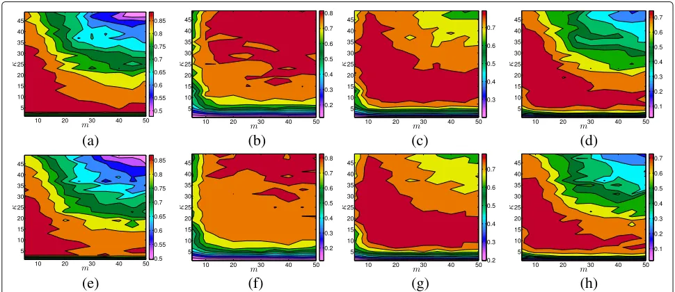
SNN similarity between SPNs, because two SPNs can only share at mostκnearest neighbors according to Eq. (3). If κis too small, even two dissimilar SPNs are likely to have a similarity ofκ and the difference between the “similar” and “dissimilar” pairs will be obscured. On the other hand, ifκis too large, the SNN similarity is insensitive to local variations, and the algorithm tends to produce large clus-ters containing the images from different actual “classes”. Similarly, ifmis too small, there will be not enough infor-mation for determining the class label of SPNs. As a conse-quence, the assigned labels remain random and unreliable, which hinders the convergence of the algorithm and result in many singleton clusters. While ifmis too large, more and more dissimilar SPNs will be involved in the cal-culation and therefore mislead the algorithm to make wrong decisions.
To see how κ and m affect the clustering quality, we applied the proposed clustering algorithm on two small subsets randomly sampled from the Dresden database. The first subset (i.e., D4 in Section 4.4.1) consists of 1000 images taken by 50 cameras, with the number of images acquired by different cameras ranging from 10 to 60, and the second subset (i.e.,D5in section 4.4.1) con-sists of 1024 images, with 24 additional singleton images (i.e., they are from 24 different cameras) added to the first subset. We varied κ from 1 to 50 and m from 5 to 50.
Results on the first and the second subset are shown in the first and second row of Fig. 2, respectively. As can be seen, ifκ is too small (e.g., < 5), the algorithm produces many small clusters and results in a very low
recall rate (see Fig. 2b, f). As κ increases, the clusters belonging to different classes are likely to be merged together, which gives rise to a lower precision rate (see Fig. 2a, e). For the size of the membership committee, a small m leads to a low recall rate (see Fig. 2a, e). As m goes up to a point where “enough” similar SPNs can help to make trustworthy decisions, it strikes a good bal-ance between the precision rate and the recall rate, and therefore achieves a favorable F1-measure and Adjusted Rand Index (see Fig. 2c, d, g, and h). But if we keep increasingm, there is a chance to decrease the precision rate (see Fig. 2a, e) due to the misleading information provided by the membership committee. The results on the first and the second subset share very similar pat-terns and trends, but the areas corresponding to high clustering quality (i.e., the areas highlighted in dark red in Fig. 2d, h) shrink towards the left-bottom corner. It indicates that a relatively smaller κ or m is prefer-able when singleton images are present in the database. In our following experiments, both κ and m are set to 15.
4.4 Comparisons and analyses
To illustrate the advantages of our proposed algorithm, we compared it with other five clustering methods: (1) the multi-class spectral clustering (SC) method [31], (2) the hierarchical clustering (HC) method [34], (3) the shared nearest neighbor clustering (SNNC) method [43], (4) the normalized cut-based clustering (NCUT) method [45], and (5) the Markov random field based clustering (MRF) method [49]. We did not include Boly’s algorithm [44] and
(a)
(b)
(c)
(d)
(e)
(f)
(g)
(h)
Marra’s algorithm [47], because both algorithms retain the fingerprints in the RAM for updating the centroids of clusters, which makes them unsuitable for relatively large datasets. Moreover, for Marra’s algorithm [47], the selec-tion ofβ, the average level of correlation for same-camera residuals, can be tricky since β varies across different cameras.
For fair comparison, we used a fully connected graph forSC rather than the sparsek-nearest neighbor graph in [31]. Also, note that we did not use the hierarchi-cal clustering proposed in [33] for comparison, because we found in experiments that the algorithm in [34] per-forms slightly faster and better than that in [33]. For SNNC, there are three parameters: the size of the nearest neighbors κ, the similarity threshold Eps for calculat-ing the SNN density, and the density threshold MinPts for finding the core points. We setκ to the same value as our proposed algorithm, i.e., κ = 15, and set Eps and MinPts to 2 and 10, respectively. For NCUT, we set the aggregation threshold Th to 0.0037 rather than the 0.037 in [45], which results in many singleton clus-ters. For MRF, to avoid going into infinite iterations when the algorithm does not converge, we set the max-imum number of iterations to 50. We will conduct two experiments, one on datasets of fixed size with vary-ing class distributions and different levels of clustervary-ing difficulty to test the adaptability of algorithms and the other on datasets of varying sizes to test thescalabilityof algorithms.
4.4.1 Clustering on datasets of fixed size
In this experiment, we first set up four datasets of fixed size and based on the Dresden database. As we know that, images acquired by cameras of the same model may undergo the same or similar image process-ing pipeline. As a result, the non-unique artifacts left in the images make them more difficult to be distin-guished from each other. We therefore categorize the clustering difficulties into easyand hard levels. For the easy level, the images in different classes are taken by cameras of different models, while on the hard level, images in some of the different classes are taken by devices of the same model. Additionally, it is common in practical situation that the numbers of images vary widely across devices. So we categorize the distribu-tions of images into symmetric and asymmetric. Based on these considerations, we set up the following four different datasets:
• D1: easy symmetric dataset, which consists of 1000 images taken by 25 cameras of different models (each accounting for 40 images). It nearly covers all the popular camera manufacturers, such as Canon, Nikon, Olympus, Pentax, Samsung, and Sony.
• D2: easy asymmetric dataset. 20, 30, 40, 50, and 60 images are alternatively selected from the images taken by each of the 25 cameras inD1to make up a total of 1000 images.
• D3: hard symmetric dataset, which consists of 1000 images taken by 50 cameras (each accounting for 20 images). The 50 cameras only cover 12 models, so some of them are of the same model.
• D4: hard asymmetric dataset. 10, 15, 20, 25, and 30 images are alternatively selected from the images taken by each of the 50 cameras inD3to make up a total of 1000 images.
Our proposed clustering algorithm essentially exploits the affinities between neighboring images. Thus, it would be interesting to see how the proposed algorithm deals with singleton classes, i.e., classes composed by only one single image as no other images from the same cam-era are present in the database. Recall that the images in our entire database are from 74 cameras and the images in dataset D4 are from 50 of them. We there-fore randomly select one image from those taken by each of the remaining 24 cameras and add them to
D4 to form an extra database, D5, consisting of 1024 images. This setting allows us to investigate the influence of singleton classes by comparing the performance on
D4andD5.
We tested the six algorithms on D1, D2, D3, D4, and D5. For each dataset, three pairwise correlation matrices are calculated using SPNs of three different sizes, namely 1024×1024, 512×512, and 512×256 pixels. The results onD1−D5are listed in Tables 1, 2, 3, 4, and 5, respec-tively. The best F1-measures, adjusted Rand Indexes, and the cluster-to-class ratios are highlighted in bold.
As can be seen, SC performs poorly on challenging datasetsD3,D4, andD5even using SPNs of 1024×1024 pixels, withF=0.18,A=0.06 in Table 3 and even worse in Tables 4 and 5. However, SC performs surprisingly bet-ter on smaller block sizes, 512×512 pixels. The rather contradictory results are due to the stop criterion of SC, because the algorithm terminates when the size of the smallest cluster equals 1. But the smallest class size of
Table 1Comparison of clustering algorithms onD1
Algorithms
1024×1024 512×512 512×256
P R F A N P R F A N P R F A N
SC [31] 0.36 0.99 0.53 0.27 0.36 0.23 0.94 0.36 0.08 0.24 0.25 0.88 0.39 0.10 0.28
HC [34] 0.71 0.57 0.63 0.54 1.24 0.94 0.18 0.30 0.72 5.20 0.87 0.10 0.19 0.49 8.40
SNNC [43] 0.90 0.48 0.63 0.77 1.88 0.63 0.23 0.34 0.42 2.68 0.59 0.19 0.29 0.35 3.08
NCUT [45] 0.86 0.16 0.27 0.65 5.44 0.73 0.24 0.36 0.51 3.08 0.68 0.24 0.36 0.48 2.80
MRF [49] 0.96 0.43 0.60 0.87 2.24 0.82 0.41 0.55 0.62 2.00 0.78 0.65 0.71 0.60 1.20
Proposed 0.99 0.80 0.88 0.93 1.24 0.93 0.83 0.88 0.84 1.12 0.86 0.72 0.78 0.72 1.20
Table 2Comparison of clustering algorithms onD2
Algorithms
1024×1024 512×512 512×256
P R F A N P R F A N P R F A N
SC [31] 0.34 0.98 0.51 0.17 0.28 0.35 0.97 0.51 0.19 0.32 0.41 0.78 0.54 0.21 0.44
HC [34] 0.82 0.58 0.68 0.63 1.48 0.50 0.77 0.61 0.28 0.68 0.85 0.14 0.24 0.59 5.60
SNNC [43] 0.88 0.48 0.62 0.76 1.80 0.60 0.19 0.29 0.37 2.80 0.54 0.16 0.24 0.27 3.16
NCUT [45] 0.86 0.20 0.33 0.71 4.28 0.75 0.30 0.43 0.61 2.56 0.72 0.38 0.50 0.58 1.76
MRF [49] 0.97 0.49 0.65 0.91 1.88 0.79 0.47 0.59 0.58 1.56 0.76 0.50 0.60 0.53 1.44
Proposed 0.97 0.78 0.86 0.91 1.20 0.92 0.87 0.89 0.87 1.04 0.88 0.83 0.85 0.78 1.04
Table 3Comparison of clustering algorithms onD3
Algorithms
1024×1024 512×512 512×256
P R F A N P R F A N P R F A N
SC [31] 0.10 1.00 0.18 0.06 0.10 0.17 0.94 0.29 0.09 0.18 0.41 0.72 0.52 0.20 0.56
HC [34] 0.71 0.50 0.58 0.44 1.44 0.81 0.21 0.33 0.52 3.92 0.76 0.13 0.22 0.31 5.94
SNNC [43] 0.45 0.26 0.32 0.23 1.74 0.35 0.15 0.21 0.11 2.34 0.30 0.12 0.17 0.07 2.50
NCUT [45] 0.92 0.13 0.22 0.52 7.30 0.72 0.14 0.24 0.37 4.96 0.53 0.15 0.23 0.25 3.58
MRF [49] 0.51 0.47 0.49 0.21 1.08 0.44 0.45 0.44 0.15 0.96 0.32 0.47 0.38 0.11 0.68
Proposed 0.87 0.75 0.80 0.74 1.16 0.68 0.64 0.66 0.48 1.06 0.52 0.47 0.49 0.16 1.10
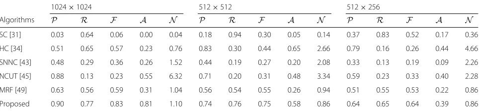
Table 4Comparison of clustering algorithms onD4
Algorithms
1024×1024 512×512 512×256
P R F A N P R F A N P R F A N
SC [31] 0.03 0.64 0.06 0.00 0.04 0.18 0.94 0.30 0.05 0.14 0.37 0.83 0.52 0.17 0.36
HC [34] 0.51 0.65 0.57 0.23 0.76 0.83 0.30 0.44 0.65 2.66 0.79 0.16 0.26 0.44 4.66
SNNC [43] 0.48 0.29 0.36 0.26 1.52 0.44 0.19 0.27 0.20 2.08 0.33 0.13 0.19 0.09 2.26
NCUT [45] 0.88 0.13 0.23 0.55 6.32 0.71 0.20 0.31 0.48 3.34 0.59 0.23 0.33 0.40 2.28
MRF [49] 0.63 0.56 0.59 0.31 1.04 0.56 0.54 0.55 0.26 0.94 0.51 0.55 0.53 0.22 0.86
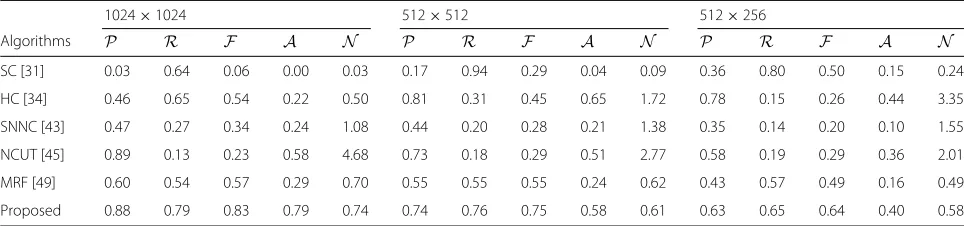
Table 5Comparison of clustering algorithms onD5
Algorithms
1024×1024 512×512 512×256
P R F A N P R F A N P R F A N
SC [31] 0.03 0.64 0.06 0.00 0.03 0.17 0.94 0.29 0.04 0.09 0.36 0.80 0.50 0.15 0.24
HC [34] 0.46 0.65 0.54 0.22 0.50 0.81 0.31 0.45 0.65 1.72 0.78 0.15 0.26 0.44 3.35
SNNC [43] 0.47 0.27 0.34 0.24 1.08 0.44 0.20 0.28 0.21 1.38 0.35 0.14 0.20 0.10 1.55
NCUT [45] 0.89 0.13 0.23 0.58 4.68 0.73 0.18 0.29 0.51 2.77 0.58 0.19 0.29 0.36 2.01
MRF [49] 0.60 0.54 0.57 0.29 0.70 0.55 0.55 0.55 0.24 0.62 0.43 0.57 0.49 0.16 0.49
Proposed 0.88 0.79 0.83 0.79 0.74 0.74 0.76 0.75 0.58 0.61 0.63 0.65 0.64 0.40 0.58
class size and easier separation of different classes, SC is able to produce much better results onD1andD2, with F = 0.53,A = 0.27 for D1and F = 0.51,A = 0.17 forD2.
The performance of HC is generally good in terms of F1-measure, but it is not as good as reported in [33] and [34], where the datasets used were less challenging in terms of both the number of cameras and the number of images captured by each camera. An interesting observa-tion is that when using SPNs of 512×512 and 512×256 pixels, HC achieves the highest precision rates in most cases. But as can be seen in Tables 1, 3, 4, and 5, the highPcomes at the expense of lowR, which means HC tends to over-partition the datasets. This is also reflected in the values of N that are much larger than 1 in the corresponding rows.
SNNC performs well on the easy datasetsD1andD2, but its performance onD3−D5is yet far from satisfactory. We found that SNNC is very sensitive to parameters. For example, if we increaseEpsfrom 2 to 4, the performance drops dramatically forD1(withF =0.40,A=0.34) and D2(withF=0.33,A=0.30). Another drawback of SNN is that it does not cluster all data points, because it dis-cards the non-core data points that are not within a radius ofEpsof a core point (i.e., the noise points in [43]). When the parameters are not set appropriately, a large fraction of data points may be identified as noise points. Taking datasetD3for example, about 25% of SPNs are identified as noise and discarded whenEpsis set to 4. However, it is difficult to determine the “right” parameters that are applicable to different datasets.
Similar to HC, NCUT tends to over-partition the datasets, which results in high precision rates, low recall rates, and cluster-to-class ratios much higher than 1. It is worth noting that there are some inconsistencies between
F andAmeasures. Taking the measures on datasetD4 using SPNs of 1024×1024 pixels (i.e., Table 3) for exam-ple, theF =0.22 of NCUT is the second worst among the six methods, but itsA=0.52 turns out to be the second best performance. The main reason is that the measure
F tends to be in favor of clusters of large granularity. To see this, let us consider clustering a dataset of 1000 images taken by 10 cameras, each responsible for 100 images. If all the 1000 images are grouped into one clus-ter, Agives a measure of 0 while F gives a measure of 0.18. If for each camera, its 80 images form a cluster and the remaining 20 images form 20 singleton clusters, thenAgives a measure of 0.76, butF only gives a mea-sure of 0.09. So F is more prone to heavily penalize singleton clusters.
By resorting to the MRF approach and the shared κ-nearest neighbor technique, our proposed algorithm is able to find high-quality clusters. Using SPNs of 1024×1024 pixels, it outperforms other five algorithms in terms of both F1-measure and adjusted Rand Index. It achievesF>=0.86,A>=0.91 on easy datasets (D1andD2) andF >=0.80,A>= 0.74 on hard datasets (D3−D5). Even using the SPNs of 512×256 pixels,F andAcan be as high as 0.72 on the two easy datasets. Compared with the MRF method in [49], the proposed algorithm shows a significantly better performance. On challenging datasets (D3−D5), the improvement can be as high as 80% (e.g., D3) and 170% (e.g.,D5) in terms ofF andA, respectively. But the 24 singleton classes added toD5do decrease the precision rate as some of the singleton classes may be wrongly attributed to the clusters close to them. One attractive feature of our proposed algorithm is that it is able to find clusters with high precision rate (i.e., high purity). The high precision rate is important and prefer-able in the context of forensic investigation, because the false attribution error (i.e., 1−P) can cause more serious problems, such as accusing an innocent person.
4.4.2 Clustering on datasets of varying sizes
covered. The six algorithms were run and evaluated on each of these datasets.
The log-scale running time (in seconds) is shown in Fig. 3. Our proposed algorithm requires the calculation of the SNN similarity before clustering, so the time used to calculate the SNN similarity is highlighted in green in the stacked bar. Since the running time obtained using SPNs of different lengths exhibit the same trend, we only show the running time for SPNs of 1024×1024 pixels. As can be observed in Fig. 3, MRF is the slowest one, followed by HC and SC. Although SC repeats spectral clustering process several times to search for the optimal number of clus-ters, the time complexity of each clustering process is only
ON32K+NK2
(K is the number of partitions), which
is lower than the time complexity O(N2logN) of HC whenN m. Our proposed algorithm is slightly slower than NCUT and SNNC but is much faster than the other three algorithms. By reducing the complexity of calcula-tion in each iteracalcula-tion and accelerating the convergence, the speed of the algorithm has been significantly improved when compared to our preliminary study in [49]. Most of the running time of our proposed algorithm is spent on constructing the SNN similarity matrix. When the SNN similarity matrix is available, the actual clustering process only takes less than 40 s (the orange bar beneath the green bar in Fig. 3) even for the dataset containing 7400 images. The clustering qualities of different algorithms are illus-trated in Fig. 4. As can be seen, our proposed algorithm performs apparently better than the other three algo-rithms in terms of both the F1-measure and adjusted Rand Index. In particular, when using the SPNs of 1024 × 1024 pixels, our proposed algorithm delivers a 23% higher F and a 13% higher A on average than the second best algorithm (see Fig. 4g, j). Its precision
rate consistently stays at a very high level (> 96%). Even using the SPNs of 512 × 256 pixels, the pre-cision rate can reach about 80%. The high prepre-cision rate makes the proposed algorithm attractive in foren-sic applications. Another important observation is that while the performances of the other five algorithms, espe-cially SC and SNNC, decline considerably in terms of
F or A when the size of the dataset increases, the performance of our proposed algorithm is quite sta-ble in terms of F, A, and N. This high stability is preferable in practice when applying the algorithm to new databases.
5 Conclusions
In this work, we have proposed a novel algorithm for clustering images taken by an unknown num-ber and unknown types of digital cameras based on the sensor pattern noises extracted from images. The clustering algorithm infers the class memberships of images from a random initial membership con-figuration in the dataset. By giving different “neigh-bors” different voting power in the concise yet effec-tive cost function depending on their similarity with the image in question, the algorithm is able to con-verge to the optimal cluster configuration accurately and efficiently. The experiments on the Dresden image database show that the proposed clustering scheme is fast and delivers very good performance. Despite the present advances, the most time-consuming step for image clustering based on SPNs is the calcu-lation of the pairwise similarity matrix due to the high dimension of SPNs. We are currently working towards formulating a compact representation of SPNs in order to facilitate the large-scale source-oriented image clustering.
(a)
(b)
(c)
(d)
(e)
(f)
(g)
(h)
(j)
(k)
(l)
(m)
(n)
(o)
(i)
Fig. 4Comparison of different clustering algorithms on datasets of varying sizes.aPrecision rates, image block sizes=1024×1024 pixels; bprecision rates,s=512×512;cprecision rates,s=512×256;drecall rates,s=1024×1024;erecall rates,s=512×512;frecall rates, s=512×256;gF1-measures,s=1024×1024;hF1-measures,s=512×512;iF1-measures,s=512×256;jadjusted Rand Indexes, s=1024×1024;kadjusted Rand Indexes,s=512×512;ladjusted Rand Indexes,s=512×256;mcluster-to-class ratios,s=1024×1024; ncluster-to-class ratios,s=512×512; andocluster-to-class ratios,s=512×256
Acknowledgements
This work is partly supported by the EU project, Computer Vision Enabled Multimedia Forensics and People Identification ( Project no. 690907; Acronym: IDENTITY), funded through the EU Horizon 2020 - Marie Skodowska-Curie Actions -Research and Innovation Staff Exchange action.
Funding
This study received funding from the EU project, Computer Vision Enabled Multimedia Forensics and People Identification (Project no. 690907; Acronym: IDENTITY), funded through the EU Horizon 2020 - Marie Skodowska-Curie Actions -Research and Innovation Staff Exchange action.
Availability of data and materials
The datasets analyzed during the current study are available in the Dresden Image Database, [http://forensics.inf.tu-dresden.de/ddimgdb/].
Authors’ contributions
iteration; and (5) accelerating the speed of convergence. Not only the presentation of the clustering methodology is more comprehensive and detailed in this work, but also the proposed algorithm is much more efficient and reliable than that in [49]. Secondly, we discuss in detail the related SPNs clustering algorithms, namely the spectral, the hierarchical, the shared nearest neighbor, the normalized cut, and our previous MRF-based clustering methods [49]. These algorithms are evaluated and compared on real-world databases to provide insight into the pros and cons of each algorithm and offer a valuable reference for practical applications. Finally, we evaluate the proposed algorithm on a large and challenging image database which contains 7400 images taken by 74 cameras, covering 27 camera models and 14 brands, while the database used in [49] includes only six cameras. Furthermore, the quality of clustering is characterized by F1-measure and adjusted Rand Index, which are more suitable for evaluating clustering results than only the true positive rate or accuracy used in [31, 33, 34, 49]. Both authors read and approved the final manuscript.
Ethical approval and consent to participate
Not applicable.
Consent for publication
Not applicable.
Competing interests
The authors declare that they have no competing interests.
Publisher’s Note
Springer Nature remains neutral with regard to jurisdictional claims in published maps and institutional affiliations.
Author details
1School of Computing and Mathematics, Charles Sturt University, Boorooma
Street, Wagga Wagga, Australia.2Department of Computer Science, University of Warwick, Gibbet Hill Road, CV4 7AL Coventry, UK.
Received: 21 April 2017 Accepted: 3 October 2017
References
1. J Lukas, J Fridrich, M Goljan, Digital camera identification from sensor pattern noise. IEEE Trans. Inf. Forensics Secur.1(2), 205–214 (2006) 2. N Khanna, GT-C Chiu, JP Allebach, EJ Delp, inProc. IEEE Int. Conf. Acoust.,
Speech, Signal Process. Forensic techniques for classifying scanner, computer generated and digital camera images, (Las Vegas, 2008), pp. 1653–1656
3. C-T Li, Source camera identification using enhanced sensor pattern noise. IEEE Trans. Inf. Forensics Secur.5(2), 280–287 (2010)
4. C-T Li, Y Li, Color-decoupled photo response non-uniformity for digital image forensics. IEEE Trans. Circ. Syst. Video Technol.22(2), 260–271 (2012) 5. X Kang, Y Li, Z Qu, J Huang, Enhancing source camera identification
performance with a camera reference phase sensor pattern noise. IEEE Trans. Inf. Forensics Secur.7(2), 393–402 (2012)
6. Y Tomioka, Y Ito, H Kitazawa, Robust digital camera identification based on pairwise magnitude relations of clustered sensor pattern noise. IEEE Trans. Inf. Forensics Secur.8(12), 1986–1995 (2013)
7. A Pande, S Chen, P Mohapatra, J Zambreno, Hardware architecture for video authentication using sensor pattern noise. IEEE Trans. Circ. Syst. Video Technol.24(1), 157–167 (2014)
8. TH Thai, R Cogranne, F Retraint, Camera model identification based on the heteroscedastic noise model. IEEE Trans. Image Process.23(1), 250–263 (2014)
9. G Chierchia, G Poggi, C Sansone, L Verdoliva, A Bayesian-MRF approach for PRNU-based image forgery detection. IEEE Trans. Inf. Forensics Secur.
9(4), 554–567 (2014)
10. S Chen, A Pande, K Zeng, P Mohapatra, Live video forensics: Source identification in lossy wireless networks. IEEE Trans. Inf. Forensics Secur.
10(1), 28–39 (2015)
11. X Lin, C-T Li, Preprocessing reference sensor pattern noise via spectrum equalization. IEEE Trans. Inf. Forensics Secur.11(1), 126–140 (2016) 12. X Lin, C-T Li, Enhancing sensor pattern noise via filtering distortion
removal. IEEE Signal Process. Lett.23(3), 381–385 (2016)
13. Y-F Hsu, S-F Chang, inProc. IEEE Int. Conf. Multimedia and Expo. Image splicing detection using camera response function consistency and automatic segmentation, (Beijing, 2007), pp. 28–31
14. AC Popescu, H Farid, Exposing digital forgeries by detecting traces of resampling. IEEE Trans. Signal Process.53(2), 758–767 (2005) 15. H Cao, AC Kot, Accurate detection of demosaicing regularity for digital
image forensics. IEEE Trans. Inf. Forensics Secur.4(4), 899–910 (2009) 16. A Swaminathan, M Wu, KR Liu, Nonintrusive component forensics of
visual sensors using output images. IEEE Trans. Inf. Forensics Secur.2(1), 91–106 (2007)
17. MJ Sorell, inProc. Int. Conf. Forensic Appl. and Tech. in Telecom., Inf. Multimedia Workshop. Conditions for effective detection and
identification of primary quantization of re-quantized jpeg images (ICST (Institute for Computer Sciences, Social-Informatics and
Telecommunications Engineering), (Adelaide, 2008), p. 18 18. K San Choi, EY Lam, KK Wong, inElectron. Imag. Source camera
identification using footprints from lens aberration (Int. Society for Optics and Photonics, San Jose, 2006), pp. 60690–60690
19. O Celiktutan, B Sankur, I Avcibas, Blind identification of source cell-phone model. IEEE Trans. Inf. Forensics Secur.3(3), 553–566 (2008)
20. G Xu, S Gao, YQ Shi, R Hu, W Su, inProc. the 8th Int. Workshop Digit. Watermarking. Camera-model identification using Markovian transition probability matrix, (2009), pp. 294–307
21. P Sutthiwan, J Ye, YQ Shi, inProc. the 8th Int. Workshop Digit. Watermarking. An enhanced statistical approach to identifying photorealistic images, (University of Surrey, Guildford, 2009), pp. 323–335
22. I Amerini, R Becarelli, B Bertini, R Caldelli, Acquisition source identification through a blind image classification. IET Image Process.9(4), 329–337 (2015)
23. R-Z Wang, Y-D Tsai, An image-hiding method with high hiding capacity based on best-block matching and K-means clustering. Pattern Recogn.
40(2), 398–409 (2007)
24. W Zhong, G Altun, R Harrison, PC Tai, Y Pan, Improved K-means clustering algorithm for exploring local protein sequence motifs representing common structural property. IEEE Trans. NanoBiosci.4(3), 255–265 (2005) 25. J Cui, J Loewy, EJ Kendall, Automated search for arthritic patterns in
infrared spectra of synovial fluid using adaptive wavelets and fuzzy c-means analysis. IEEE Trans. Biomed. Eng.53(5), 800–809 (2006) 26. D Dembélé, P Kastner, Fuzzy c-means method for clustering microarray
data. Bioinformatics.19(8), 973–980 (2003)
27. NR Pal, K Pal, JM Keller, JC Bezdek, A possibilistic fuzzy c-means clustering algorithm. IEEE Trans. Fuzzy Syst.13(4), 517–530 (2005)
28. B Hendrickson, RW Leland, A multi-level algorithm for partitioning graphs. Supter Comput.95, 28 (1995)
29. G Karypis, V Kumar, A fast and high quality multilevel scheme for partitioning irregular graphs. SIAM J. Sci. Comput.20(1), 359–392 (1998) 30. U Von Luxburg, A tutorial on spectral clustering. Stat. Comput.17(4),
395–416 (2007)
31. B Liu, H-K Lee, Y Hu, C-H Choi, inProc. IEEE Int. Workshop Inf. Forensics Security. On classification of source cameras: A graph based approach, (Seattle, 2010), pp. 1–5
32. SX Yu, J Shi, inProc. IEEE Int. Conf. Comput. Vision. Multiclass spectral clustering, (Nice, 2003), pp. 313–319
33. R Caldelli, I Amerini, F Picchioni, M Innocenti, inProc. IEEE Int. Workshop Inf. Forensics Security. Fast image clustering of unknown source images, (Seattle, 2010), pp. 1–5
34. LJG Villalba, ALS Orozco, JR Corripio, Smartphone image clustering. Expert Syst. with Appl.42(4), 1927–1940 (2015)
35. S Guha, R Rastogi, K Shim, inACM SIGMOD Record. Cure: an efficient clustering algorithm for large databases, vol. 27 (ACM, Seattle, 1998), pp. 73–84
36. S Guha, R Rastogi, K Shim, inProc. Int. Conf. Data Eng. Rock: A robust clustering algorithm for categorical attributes (IEEE, Sydney, 1999), pp. 512–521
37. G Karypis, E-H Han, V Kumar, Chameleon: Hierarchical clustering using dynamic modeling. Computer.32(8), 68–75 (1999)
38. R Xu, D Wunsch, Survey of clustering algorithms. IEEE Trans. Neural Netw.
16(3), 645–678 (2005)
40. C-T Li, R Satta, Empirical investigation into the correlation between vignetting effect and the quality of sensor pattern noise. IET Comput. Vision.6(6), 560–566 (2012)
41. M Ester, H-P Kriegel, J Sander, X Xu, et al, inProc. ACM SIGKDD Int. Conf. Knowl. Discovery Data Mining. A density-based algorithm for discovering clusters in large spatial databases with noise, vol. 96, (Portland, 1996), pp. 226–231
42. A Hinneburg, DA Keim, inProc. ACM SIGKDD Int. Conf. Knowl. Discovery Data Mining. An efficient approach to clustering in large multimedia databases with noise, vol. 98, (New York, 1998), pp. 58–65 43. L Ertöz, M Steinbach, V Kumar, inProc. Int. Conf. Data Mining. Finding
clusters of different sizes, shapes, and densities in noisy, high dimensional data (SIAM, San Francisco, 2003), pp. 47–58
44. GJ Bloy, Blind camera fingerprinting and image clustering. IEEE Trans. Pattern Anal. Mach. Intell.30(3), 532–534 (2007)
45. I Amerini, R Caldelli, P Crescenzi, AD Mastio, A Marino, Blind image clustering based on the normalized cuts criterion for camera identification. Signal Process. Image Commun.29(8), 831–843 (2014) 46. J Shi, J Malik, Normalized cuts and image segmentation. IEEE Trans.
Pattern Anal. Mach. Intell.22(8), 888–905 (2000)
47. F Marra, G Poggi, C Sansone, L Verdoliva, inProc. Int. Workshop on Inf. Forensics and Security (WIFS). Correlation clustering for prnu-based blind image source identification, (Abu Dhabi, 2016), pp. 1–6
48. N Bansal, A Blum, S Chawla, Correlation clustering. Mach. Learn.56(1-3), 89–113 (2004)
49. C-T Li, inProc. IEEE Int. Symp. Circuits Syst. Unsupervised classification of digital images using enhanced sensor pattern noise, (Paris, 2010), pp. 3429–3432
50. K Dabov, A Foi, V Katkovnik, K Egiazarian, Image denoising by sparse 3-d transform-domain collaborative filtering. IEEE Trans. Image Process.16(8), 2080–2095 (2007)
51. RA Jarvis, EA Patrick, Clustering using a similarity measure based on shared near neighbors. IEEE Trans. Comput.100(11), 1025–1034 (1973) 52. T Gloe, S Pfennig, M Kirchner, inProc. ACM Workshop Multimedia Security.
Unexpected artefacts in PRNU-based camera identification: a ’Dresden Image Database’ case-study, (Coventry, 2012), pp. 109–114
53. R Wilson, C-T Li, A class of discrete multiresolution random fields and its application to image segmentation. IEEE Trans. Pattern Anal. Mach. Intell.
25(1), 42–56 (2003)
54. C-T Li, Multiresolution image segmentation integrating gibbs sampler and region merging algorithm. Signal Process.83(1), 67–78 (2003) 55. M Vignes, F Forbes, Gene clustering via integrated Markov models
combining individual and pairwise features. IEEE/ACM Trans. Comput. Biol. Bioinf.6(2), 260–270 (2009)
56. X Zhang, X Hu, X Hu, E Park, X Zhou, Utilizing different link types to enhance document clustering based on Markov Random Field model with relaxation labeling. IEEE Trans. Syst. Man Cybern. Part A: Syst. Humans.
42(5), 1167–1182 (2012)
57. AL Varna, M Wu, inProc. IEEE Int. Workshop Inf. Forensics Security. Modeling content fingerprints using Markov random fields, (London, 2009), pp. 111–115
58. C Martınez, inProc. ACM-SIAM Workshop on Algorithm Engineering and Experiments and 1st ACM-SIAM Workshop on Analytic Algorithmics and Combinatorics. Partial quicksort, (New Orleans, 2004), pp. 224–228 59. X Lin, CT Li, Large-scale image clustering based on camera fingerprints.
IEEE Trans. Inf. Forensics Security.12(4), 793–808 (2017)
60. T Gloe, R Böhme, The Dresden image database for benchmarking digital image forensics. J. Digit. Forensic Practice.3(2-4), 150–159 (2010) 61. WM Rand, Objective criteria for the evaluation of clustering methods.
J. Am. Stat. Assoc.66(336), 846–850 (1971)