http://www.sciencepublishinggroup.com/j/ajnna doi: 10.11648/j.ajnna.20190502.12
ISSN: 2469-7400 (Print); ISSN: 2469-7419 (Online)
Application of Group Method of Data Handling Type Neural
Network for Significant Wave Height Prediction
Moussa Sobh Elbisy, Faisal Abdulrahman Osra
Civil Engineering Department, Umm Al Qura University, Makkah, Saudi Arabia
Email address:
To cite this article:
Moussa Sobh Elbisy, Faisal Abdulrahman Osra. Application of Group Method of Data Handling Type Neural Network for Significant Wave Height Prediction. American Journal of Neural Networks and Applications. Vol. 5, No. 2, 2019, pp. 51-57.
doi: 10.11648/j.ajnna.20190502.12
Received: October 5, 2019; Accepted: October 22, 2019; Published: October 28, 2019
Abstract:
The estimation of wave parameters is of great importance in coastal activities such as design studies for harbor, inshore and offshore structures, coastal erosion, sediment transport, and wave energy estimation. For this purpose, several models and approaches have been proposed to predict wave parameters, such as empirical, numerical-based approaches, and soft computing. In this study, the group method of data handling type neural network (GMDH-NN) was presented for significant wave height prediction in an attempt to suggest a new model with superior explanatory power and stability. The GMDH-NN results were compared with the field data and with a multilayer perceptron neural networks (MLPNN) model. The results indicate that the prediction accuracy and avoidance of over-fitting of the GMDH-NN method were superior to those of the MLPNN method. The percentage improvement in the root mean square error and the mean absolute percentage error of the GMDH-NN model over the MLPNN model were 72.92% and 81.02%, respectively. Also, according to the indices, the GMDH-NN model performs the best for predicting the Hs of all of the wave height ranges. That is, the GMDH-NN model is capable of predicting wave heights for different ranges. The results of the analysis suggest that the GMDH-NN-based modeling is effective in predicting significant wave height.Keywords:
Significant Wave Height, Prediction, Group Method of Data Handling, Multilayer Perceptron1. Introduction
Waves are important factors in the planning and design of harbors, waterways, shore protection projects, and offshore structures, as well as for environmental impact assessments and hazard mitigation. The field observation of waves is generally difficult, and the numerical modelling of waves is costly and time consuming. Various methods, such as empirical, numerical, and soft computing approaches, have been proposed in the literature for wave parameter prediction.
The most commonly used soft computing techniques that has been proposed to forecast wave parameters is the neural networks (NNs). Deo and Naidu [1] compared the forecasting results of NNs and auto-regressive models and reported that NN models are more accurate. Deo et al. [2] tested a feed-forward neural network (FFNN) to obtain significant wave heights and average wave periods by using the current and previous time step wind speed values as
perform nearly the same. According to the meteorological data, Günaydın [9] predicted monthly mean significant wave heights by using NN and regression methods. On the other hand, Elbisy [10] used the support vector machine (SVM) approach with various kernel functions for wave parameters prediction. The SVM results were compared with the field data and BPNN and CCNN models, and the results indicated that the SVM with a radial basis function kernel provides the best generalization capability and the lowest prediction error. While Malekmohamadi et al. [11], Londhe et al. [12], and Deshmukh et al. [13] combined NN and numerical models to realize the wave height prediction, Sadeghifar et al. [14] used recurrent neural networks (RNN) for wave predictions based on the data gathered and the measurement of the sea waves in the Caspian Sea in the north of Iran. Additionally, Elgohery et al. [15] used nonlinear regression and SVM methods to predict significant wave height. The results explained that the use of nonlinear regression methods gave a good result as compared to the results from the SVM; However, the results also indicated that the SVM based on radial basis function is more superior to the nonlinear regression methods.
The aim of the present study is to illustrate a new approach to predict significant wave height using the group method data handling type neural network (GMDH-NN). The performances of GMDH-NN is evaluated by the multi-layer perceptron neural network (MLPNN).
The group method of data handling (GMDH) type neural network (NN) is a powerful identification technique and can be used to model complex systems where unknown relationships exist between the variables without having specific knowledge of the processes. GMDH is a kind of machine learning algorithm where an artificial neural network algorithm is built heuristically using the self-organization method. Originally, GMDH-NN s were applied to predict and forecast a univariate time series. But now, GMDH finds its applications in a wide spectrum of areas, such as prediction, forecasting, data mining, systems modelling, pattern recognition and knowledge discovery. GMDH-NN algorithms are generally inductive and offer the possibility to manage interrelations among data automatically. Its most powerful feature is the ability to select the optimal complexity of the neural network structure while achieving the maximum possible prediction accuracy. Once the optimal complexity of the neural network structure is found, the prediction model is quite resistant to noise in the data sample. In data mining, the model avoids overfitting and underfitting, where the noise in the data would no longer pose the problem of performance degradation. Therefore, the neural network structure is simplified and yields an optimal model that is just sufficient in the number of neurons and hidden layers to maintain its maximum possible accuracy.
The manuscript is organized in the following manner: the next section introduces the methods used in this study. Section 3 describes the studied area and the data used.
Section 4 presents the results of the GMDH-NN and MLPNN methods, and the conclusions are reported in the final section.
2. Wave Prediction Methods
2.1. Group of Method of Data Handling Type Neural Network
The concept of neural networks (NN) was inspired by the complex architecture of the human brain, which is regarded to be a highly non-linear, parallel operating system [16]. The group method of data handling type neural network (GMDH-NN) is a self-organizing approach by which gradually complicated models are generated based on the evaluation of their performances on a set of multi-input single-output data pairs (Xi, yi) (= 1, 2,…, M). The main idea of GMDH is to
build an analytical function in a feed forward network based on a quadratic node transfer function whose coefficients are obtained using the regression technique. Using the GMDH algorithm, a model can be represented as a set of neurons in which the different pairs in each layer are connected through a quadratic polynomial and produce new neurons in the next layer. Such representations can be used to map inputs to outputs [17]. The formal definition of the identification problem is to find a function that can be used approximately instead of the actual one in order to predict output for a given input vector = , , , … . . , as closely as possible to the actual output y. Therefore, given M
is the observation of multi-input-single-output data pairs,
= , , , … . . , , (i=1, 2, 3, …., M) (1) It is now possible to train a GMDH-NN to predict the output values for any given input vector =
, , , … . . , , that is,
= , , , … . . , , (i=1, 2, 3, …., M) (2) In order to determine a GMDH-NN, the square of the differences between the observed and predicted output one was minimized, that is:
∑ , , , … . . , − → (3) The general connection between the input and output variables can be expressed by a complicated discrete form of the Volterra functional series in the form of:
=
+ ∑ + ∑ ∑ +
∑ ∑ ∑ + ⋯ (4)
This is known as the Kolmogorov-Gabor polynomial. The full form of this mathematical description can be represented by a system of partial quadratic polynomials consisting of only two variables (neurons) in the form of [18]:
= !" , # = + + + + $ + % (5)
recursively used in a network of connected neurons to build the general mathematical relation between the inputs and output given in (4). The coefficients ai in (5) are calculated using regression techniques to minimize the difference between the observed output y, and the calculated one, for each pair of xi, xj as input variables. Apparently, a tree of polynomials is constructed using the quadratic form given in (5) whose coefficients are obtained in a least squares scheme [19].
In this way, the coefficients of each quadratic function Gi are obtained to optimally fit the output in the whole set of input–output data pairs, that is
& =∑0)12'()*+)",),,-#./→ min
(6)
In the basic form of the GMDH algorithm, all the possibilities of the two independent variables out of the total n input variables are taken in order to construct the regression polynomial in the form of (5) that best fits the dependent observations (yi = 1, 2,..., M) in a least squares sense [20].
Using the quadratic sub-expression in the form of (5) for each row of M data triples, the following matrix equation can be readily obtained as
6 = (7) where a is the vector of unknown coefficients of the quadratic polynomial in (5):
6 = 7 , , , , $, %8 (8) And:
= 7 , , , $, %89 (9)
Here, y is the vector of the output’s value from observation. It can be readily seen that:
6 =11 ;; <<
1 ; <
; < ; <
; < ; <
; < ; <
(10)
The least squares technique from the multiple regression analysis leads to the solution of the normal equations in the form of:
= 696 * 69 (11)
This determines the vector of the best coefficients of the quadratic (3) for the whole set of M data triples. This procedure is repeated for each neuron of the next hidden layer according to the connectivity topology of the network. When the errors for the test data in each layer stop decreasing, the iterative computation is terminated.
2.2. Multi - Perceptron Neural Network
As the name implies, an MLPNN can have several layers. Each layer has a weight matrix, a bias vector, and an output vector. The MLPNN architecture contains an input layer, an
output layer, and at least one hidden layer, which are fully interconnected. The network is repeatedly exposed to a set of training data, and errors are calculated based on the resulting outputs. These errors are used to adjust the weights and biases. This process will eventually lead to optimum and bias values that can mimic the model. The transfer functions (logistic [sigmoid] and linear) are used as an activation function for the hidden layers and the output layer, respectively. A wide range of parameters, such as the number of layers and neurons of each layer, initial conditions and learning factors, can affect the network’s performance.
3. Study Area and Data
The study area is the Abu Qir Bay coastal zone, which is a semi-circular basin that lies approximately 35 km northeast of Alexandria on the north-eastern Egyptian Nile delta coast between latitude 31°16' and 31°28'N and longitude 30°4' and 30°20'E. The bay has a shoreline length of approximately 50 km. It is relatively shallow with a depth of less than one metre along the coast that increases gradually away from the shore to reach a maximum depth of approximately 15 m.
The wind data (speed and direction), which was taken during 2010–2014 from a weather station at the Abu Qir Bay, were sampled at 6-hour intervals and calculated at 10 m above sea level. The collected wind data were subjected to statistical analysis to determine the percentage of occurrence of a certain wind speed moving in a certain direction.
The mean monthly wind speed is lower in summer and higher in winter due to frequent storms during the winter season: speeds of average 2 knots could be seen in the summer and spring months and 4 knots in winter. The maximum mean wind speed (8.5 knots) occurred in December, while the minimum (1.5 knots) was in August. The wind observations reveal that the winter season is characterised by winds coming from all directions; however, northerly and northwesterly winds are still more predominant than those from the other directions.
The waves were measured using a Cassette Acquisition System (CAS) directional wave recorder during 2010–2014. The data were statistically analysed in terms of directional and wave height distributions. Approximately 87% of all wave heights were less than or equal to 1.5 m, and 13% were greater than this value. The average annual wave height was approximately 0.94 m, and the predominant direction of all waves was from the NW (42%) with a portion (25%) approaching from the WNW. The majority of the wave period values (59%) ranged between 5 and 8 s with an annual mean period of 6.5 s. Additionally, for all of the waves, approximately 80% of wave periods were less than or equal to 8 s. The maximum significant wave height (4.19 m) was observed during the winter season with a wave period of 10.7 s and it came from the NW.
4. Results and Discussion
input variables to the GMDH-NN and MLPNN models. The output was the significant wave height (Hs). The agreement between the predictions and the observations can be checked statistically by calculating the following measures: the normalized mean square error (NMSE), the correlation coefficient (R), the root mean square error (RMSE), the mean squared error (MSE), the mean absolute error (MAE), and the mean absolute percentage error (MAPE).
=>?& =@∑ A)*B) /
ACBC
@ (12)
D = ∑E)12'A)*AC.'B)*BC. F∑ 'AE)12 )*AC./∑E)12'B)*BC./ (13)
D>?& = F@∑@ G − H (14)
>?& =@∑@ G − H (15)
>6& =@∑ |G − H |@ (16)
>6G& = J@∑ KA)*B) A) K @ L M100 (17)
where Oiis the observed value, Pi is the predicted value, N is the total number of data points in validation, O − is the mean value of the observations, and P − is the mean value of the predictions. Further, the RMSE describes the average difference between the predicted value and measured value, the MAE shows how developed models overestimate or underestimate the measured values, the MAPE describes the accuracy of the models by error percentage, the R describes the degree of association between the predicted and the measured values, and the NMSE statistics indicates that the model performance over the entire data set of sampled concentrations are not fulfilled. The MSE is a common measure of model quality. A certain amount of data processing is required before presenting the training patterns to the network. In this study, a linear scaling was used. A linear normalization function within the values of zero to one is as follows: ? O OP ⁄ OPQ, OP (18)
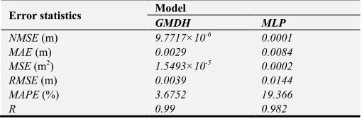
where S is the normalized value of variable V, and Vmin and Vmax are the variable minimum and maximum values, respectively. In this study, MLPNN was used as a benchmark, and a genetic algorithm (GA) was utilised to adjust the MLPNN model to its optimised performance. The GA tests the different combinations of the different parameters. This process is repeated for each solution in a generation so that new generations that are ameliorated are compared to their predecessors. The network parameters tested in the proposed model included the following: the number of hidden layers, the number of hidden neurons, the learning rate, the momentum factor, the input noise, and the training time. The integrated performance testing indicated the following best network parameters: the number of hidden layers was two, the number of neurons in the first hidden layer was two, the number of neurons in the second hidden layer was seventeen, the learning rate was 0.75, the momentum factor was 0.31, and the input noise was 0.016. The model results for different MLPNN architectures are presented in Figure 1, which shows the performance of the MLPNN with various neurons in one hidden layer. Figure 1. The performance of the MLPNN with a number of neurons in a hidden layer. Table 1 shows the error statistics for the observed and predicted significant wave heights. The values for the NMSE, MAE, MSE, RMSE, MAPE and R of the wave height MLPNN prediction model are 0.0001 m, 0.00836 m, 0.00021 m2, 0.01441 m, 19.366, and 0.99, respectively. The results show that the MLP model significantly reduces the overall error. The correlation between the observed and predicted values for Hs by the MLP model is shown in Figure 2. Figure 3 presents the residual error between the observed and predicted Hs for the MLP (2–17–1) model. Table 1. Error statistics for the observed and predicted Hs by the GMDH-NN and MLPGMDH-NN models. Error statistics Model GMDH MLP NMSE (m) 9.7717×10⁻⁶ 0.0001 MAE (m) 0.0029 0.0084 MSE (m2) 1.5493×10⁻⁵ 0.0002 RMSE (m) 0.0039 0.0144 MAPE (%) 3.6752 19.366 R 0.99 0.982 As mentioned in the GMDH-NN definitions section, the structure of the GMDH model is built using the least square sense. In the present study, the Quadratic polynomial neurons extracted from the GMDH model were expressed as: ST 0.646734 0.000615Z 0.000051Z 0.618327] 0.148482] 0.001129Z] (19) When the GMDH-NN model was applied, the NMSE was 9.7717×10⁻⁶, the MAE was 0.002879, the MSE was 1.54931×10⁻⁵, the RMSE was 0.003936, and the MAPE was 3.6752. Following this, a correlation coefficient of 0.999 was obtained. The results show that the GMDH-NN model significantly reduces overall error. The variation in Hs
model has the same trend. Figure 4 illustrates the residual error between the observed and predicted Hs for the GMDH-NN model. The correlation between the observed and predicted values for Hs by the GMDH-NN model is shown in
Figure 5.
Figure 2. Scatter of the predicted and observed values of Hs for the MLPNN model.
Figure 3. The residual error between the observed and predicted Hs for the MLPNN model.
Figure 4. The residual error between the observed and predicted Hs for the GMDH-NN model.
Figure 5. The scatter of the predicted and observed values of Hs for the GMDH-NN model.
According to the indices, the GMDH-NN model can significantly reduce the overall forecasting errors, produce the best performance, and accurately estimate the wave heights. A comparison of the results of the GMDH-NN model and the MLPNN model shows that the percentage improvements in the MAE, RMSE, and MAPE of the GMDH-NN model over the MLPNN model were 65.48%, 72.92%, and 81.02% for predicting Hs, respectively.
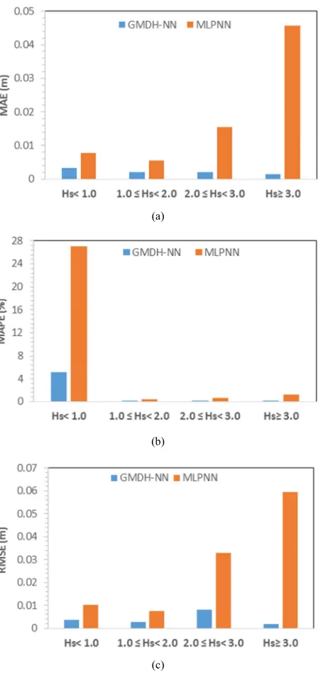
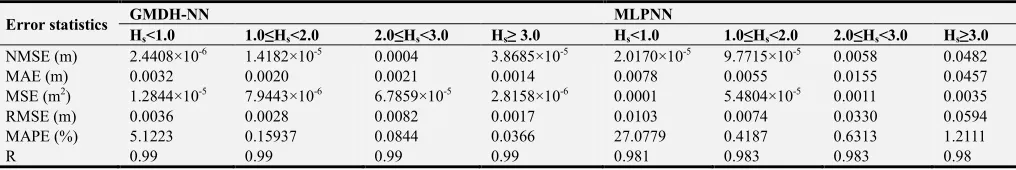
The prediction accuracies of the GMDH-NN model and the MLPNN model for different wave height ranges were investigated. Table 2 shows that the GMDH-NN performed better than the MLPNN. According to the indices, the GMDH-NN model performed the best in terms of predicting Hs for all of the wave height ranges.
(a)
(b)
(c)
A comparison of the MAE values shows that the largest difference in the performance of the two methods, 96.94%, was observed at wave heights of more than 3.0 m, while the smallest difference (58.97%) was observed at wave heights of less than 1.0 m (Figure 6a). From Figure 6b, the largest performance difference, in terms of MAPE, for the two methods (96.98%) was observed at wave heights of more than 3.0 m, while the smallest difference (61.94%) was observed at wave heights from 1.0 to 2.0 m.
A comparison of the RMSE values shows that the largest difference in the performance of the two methods (97.14%) was observed at wave heights of more than 3.0 m, while the
smallest difference (62.16%) was observed at wave heights from 1.0 to 2.0 m (Figure 6c). From the results, it can be seen that the predictions of the GMDH-NN were closer to the corresponding actual values at all wave height ranges than for the MLPNN method. Generally, the GMDH-NN model forecasting results are more accurate than of the MLPNN. That is, the GMDH-NN model is capable of forecasting wave heights of different ranges. The notable point in this method is the self-organizing characteristic of the network and its high flexibility, making it a powerful instrument for the prediction of a variety of nonlinear complex systems.
Table 2. The Error statistics for the observed and predicted Hs by the MLPNN and GMDH-NN models for different height ranges.
Error statistics GMDH-NN MLPNN
Hs<1.0 1.0≤Hs<2.0 2.0≤Hs<3.0 Hs≥ 3.0 Hs<1.0 1.0≤Hs<2.0 2.0≤Hs<3.0 Hs≥3.0
NMSE (m) 2.4408×10⁻⁶ 1.4182×10⁻⁵ 0.0004 3.8685×10⁻⁵ 2.0170×10⁻⁵ 9.7715×10⁻⁵ 0.0058 0.0482
MAE (m) 0.0032 0.0020 0.0021 0.0014 0.0078 0.0055 0.0155 0.0457
MSE (m2) 1.2844×10⁻⁵ 7.9443×10⁻⁶ 6.7859×10⁻⁵ 2.8158×10⁻⁶ 0.0001 5.4804×10⁻⁵ 0.0011 0.0035
RMSE (m) 0.0036 0.0028 0.0082 0.0017 0.0103 0.0074 0.0330 0.0594
MAPE (%) 5.1223 0.15937 0.0844 0.0366 27.0779 0.4187 0.6313 1.2111
R 0.99 0.99 0.99 0.99 0.981 0.983 0.983 0.98
5. Conclusions
The sea waves parameters’ prediction problems play an important role in many different ocean engineering tasks, such as the designing of marine structures like oil platforms or harbors or in the designing and management of marine energy systems, such as the proper operation of wave energy converters, among others [21-22]. The group method of data handling type neural network (GMDH-NN) was implemented in this investigation to predict the significant wave height using wind speed and fetch data. The GMDH-NN model results were compared with the field data and with the MLPNN model. The results show that the accuracies of the models obtained using these two methods were quite high. The GMDH-NN model (NMSE=9.7717×10⁻⁶, MAE=0.0029, MSE=1.5493×10⁻⁵,
RMSE=0.0039, MAPE=3.6752, and R=0.99) performed better than the MLP model (NMSE=0.0001, MAE=0.0084, MSE=0.0002, RMSE=0.0144, MAPE=19.366, and R=0.982) in all respects. A comparison of the significant wave height prediction results obtained with the GMDH-NN model and those obtained with the MLPNN model showed 65.48%, 72.92%, and 81.02% improvements in the MAE, RMSE, and
MAPE, respectively, using the GMDH-NN model. Also, according to the indices, the GMDH-NN model performs the best for predicting the Hs of all of the wave height
ranges. That is, the GMDH-NN model is capable of forecasting wave heights for different ranges. In conclusion, the GMDH-NN model was demonstrated to be the more efficient and robust of the two models for use in predicting significant wave height.
Acknowledgements
The authors would like to express his high appreciation to the referees of the paper for their critical review as well as their valuable comments that improved the paper to its present form.
References
[1] Deo, M. C., and Naidu, C. S. (1999). “Real time wave forecasting using neural networks.” Ocean Engineering, Vol. 26, pp. 191-203. [2] Deo, M. C.; Jha, A., Chaphekar, A. S., and Ravikant, K. (2001). “Neural networks for wave forecasting.” Ocean Engineering, Vol. 28, pp. 889–898.
[3] Agrawal, J. D. and Deo, M. C. (2002). “On-line wave prediction.” Marine Structures, Vol. 15, pp. 57–74.
[4] Tsai, C. P., Lin, C., and Shen, J. N. (2002). “Neural network for wave forecasting among multi-stations.” Ocean Engineering, Vol. 29, pp. 1683-1695.
[5] Makarynskyy, O. (2004). “Improving wave predictions with artificial neural networks.” Ocean Engineering, Vol. 31, No. 5–6, pp. 709–724.
[6] Makarynskyy, O., Pires-Silva, A. A., Makarynska, D., and Ventura-Soares, C. (2005). “Artificial neural networks in wave predictions at the west coast of Portugal.” Comput. Geosci., Vol. 31, No. 4, pp. 415–424.
[7] Mandal, S., and Prabaharan, N. (2006). “Ocean wave forecasting using recurrent neural networks.” Ocean Engineering, Vol. 33, pp. 1401–1410.
[9] Günaydın, K. (2008). “The estimation of monthly mean significant wave heights by using artificial neural network and regression methods.” Ocean Engineering, Vol. 35, pp. 1406– 1415.
[10] Elbisy, M. S. (2015). “Sea wave parameters prediction by support vector machine using a genetic algorithm.” Journal of Coastal Research, Vol. 31, No. 4, pp. 892-899.
[11] Malekmohamadi, I., Ghiassia, R., and Yazdanpanah, M. J. (2008). “Wave hindcasting by coupling numerical model and artificial neural networks.” Ocean Engineering, Vol. 35, pp. 417–425
[12] Londhe, S. N., and Panchang, V. (2016). “One-day wave forecasts based on artificial neural networks.” J. Atmos. Oceanic Tech- nol., Vol. 23, pp. 1593–1603.
[13] Deshmukh, A. N., Deo, M. C., Bhaskaran, P. K., Balakrishnan Nair, T. M., and Sandhya K. G., (2016). “Neural-network-based data assimilation to improve numerical ocean wave forecast.” IEEE J. Oceanic Eng., Vol. 41, pp. 944–953. [14] Sadeghifar, T., Motlagh, M. N., Azad, M. T., and Mahdizadeh,
M. M. (2017). “Coastal wave height prediction using Recurrent Neural Networks (RNNs) in the South Caspian Sea.” Marine Geodesy, Vol. 40, No. 2, pp. 454-465.
[15] Elgohary, T., Elbisy, M. S., Mobasher, A. M., and Salah, H. (2018). “Deep wave height prediction for Alexandria sea region by using nonlinear regression method compared to support vector machines.” Current Development in Oceanography, Vol. 10, No. 1, pp. 1-14.
[16] Haykin, S. (1999). “Neural networks: A comprehensive foundation.” New Jersey, NJ: Prentice Hall.
[17] Garg, V. (2014). “Inductive group method of data handling neural network approach to model basin sediment yield.” J Hydrol Eng, Vol. 20, No. 6, C6014002.
[18] Kalantary, F., Ardalan, H, and Nariman-Zadeh, N. (2009). “An investigation on the Su–NSPT correlation using GMDH type neural networks and genetic algorithms.” Eng Geol, Vol. 104, No. 1–2, pp. 44–55.
[19] Amanifard, N., Nariman-Zadeh, N., Farahani, M. H., and Khalkhali, A. (2008). “Modeling of multiple short-length-scale stall cells in an axial compressor using evolved GMDH neural networks,” Energy Conversion and Management, vol. 49, No. 10, pp. 2588–94.
[20] Nariman-Zadeh, N., Darvizeh, A., Felezi, M. E., and Gharababaei, H. (2002). “Polynomial modelling of explosive compaction process of metallic powders using GMDH-type neural networks and singular value composition.” Model. Simul. Mater. Sci. Eng., Vol. 10, No. 6, pp. 727-744.
[21] Comola, F., Lykke Andersen, T., Martinelli, L., Burcharth, H. F., and Ruol, P.(2014). “Damage pattern and damage progression on breakwater roundheads under multidirectional waves.” Coastal Engineering, Vol. 83, pp. 24–35.