Decision Optimization for Power Grid Operating Condition with High and Low Voltage Parallel Loops

Article

Decision Optimization for Power Grid Operating

Condition with High and Low Voltage Parallel Loops

Dong Yang 1_{, Kang Zhao} 1_{, Hao Tian} 2 _{and Yutian Liu} 2,_*

1 _{State Grid Shandong Electric Power Research Institute; Jinan 250003, China; [email protected]}

2 _{Key Laboratory of Power System Intelligent Dispatch and Control of Ministry of Education, Shandong}

University; Jinan 250061, China; [email protected]

* Correspondence: [email protected]; Tel.: +86-0531-81696103

Abstract: With the development of higher voltage power grid, the high and low voltage parallel loops are emerging, which lead to energy losses, even threaten the security and stability of power system. The multi-infeed HVDC configurations widely appearing in AC/DC interconnected power system make this situation even worse. Aimed at energy saving and system security, a decision optimization method for power grid operating condition with high and low voltage parallel loops is proposed in this paper. Firstly, considering hub substation distribution and power grid structure, parallel loop opening schemes are generated with GN algorithm. Then, candidate opening schemes are preliminarily selected from all these generated schemes based on a filtering index. Finally, with the influence on power system security, stability and operation economy in consideration, an evaluation model for candidate opening schemes is founded based on analytic hierarchy process (AHP). And a fuzzy evaluation algorithm is used to find the optimal scheme. Simulation results of New England 39-bus system and an actual power system validate the effectiveness and superiority of this proposed method.

Keywords: parallel loop; line switching; complex network theory; GN algorithm; comprehensive evaluation model

1. Introduction

The high and low voltage parallel loop is a kind of power grid structure, in which transmission lines of different voltage levels are looped by transformers in the sending and receiving end. With the rapid development of higher voltage power grid, parallel loops [1] become more and more common. Parallel flow in parallel loop would make unbalanced power flow in power system, which leads to higher power losses. In some cases, parallel loop would even threaten the security and stability of power system [2]. On the one hand, low-voltage transmission lines of parallel loops would bear a quite heavy load after faults on high-voltage transmission lines, which may cause cascading trips of low-voltage transmission lines [3]. On the other hand, parallel operation of high and low voltage transmission lines also leads to a high level of short circuit current, which may exceed the interrupting capacity of circuit breaker. Therefore, considering energy saving and system security and stability, some methods must be presented to solve these problems.

problem, which is multi-objective, non-linear and discrete. In order to simplify the calculation complexity, the decision process of opening parallel loops is usually divided into two stages: scheme generation and scheme evaluation.

The generation of opening schemes used to only depend on engineering experience. But things are changing gradually. There are researches employing linear programming algorithm to find the optimal line switching scheme with minimum power losses [11,12]. These researches only consider the branch active power flow constraint, and the bus voltage constraint is neglected. Simulation results in [13] show that the neglect of bus voltage constraint may cause the failure of optimization. A line switching optimization method considering bus voltage constraint is proposed in [14], which could effectively eliminate over-limited power flows. In [15], the Benders decomposition technology is applied to network reconfiguration, which could deal with the constraints of static security and transient stability simultaneously. But this method is barely able to be used in actual large-scale power system for its high complexity.

The evaluation of opening schemes should consider static security, transient stability, short circuit current and operation economy of power system. A comprehensive evaluation method for opening schemes is proposed in [16], which combines AHP with fuzzy evaluation algorithm. The AHP is used to establish the hierarchical model to describe the operation characteristics of power system. In this model, five performance indices and corresponding membership functions are presented. After detailed analysis and calculations for each opening scheme, the optimal one is obtained by two-level fuzzy evaluation.

All of the previous researches only discuss parallel loop opening issues in pure AC power grid. But things in AC/DC interconnected power grid would be quite different, usually more complicated indeed. Due to intensive loads in relatively narrow region, several HVDC inverter stations would emerge in adjacent area of the same AC power grid, called the multi-infeed HVDC configuration. In this situation, switching transmission lines, on the one hand, would decrease short circuit current, on the other hand, would stretch the electrical distance between different HVDC inverter stations. As a result, the multi-infeed short-circuit ratio (MISCR) may be increased or decreased under different conditions, which means the stability of power system would be influenced [17]. Therefore, the decision for the optimal parallel loop opening scheme must consider the support ability for HVDCs, which is evaluated by MISCR.

In order to solve the parallel loop problem not only in pure AC power grid but also in AC/DC interconnected power grid, a decision optimization method is proposed in this paper. In section 2, the complex network theory used for opening parallel loops is discussed in detail. GN algorithm and modularity indicator are introduced. In section 3, the generation process of candidate opening schemes is proposed. The weighted modularity indicator and weighted MISCR are defined respectively, and combined to filter generated opening schemes. In section 4, an evaluation model for candidate schemes is founded based on AHP, which considers the relationship between stability and short circuit current level of power system. A fuzzy evaluation algorithm is used to find the optimal opening scheme. In section 5, New England 39-bus system and an actual power system are analyzed. Simulation results validate the effectiveness and superiority of this proposed method.

2. Complex Network Theory Used for Opening Parallel Loops

2.1. Complex Network Complexity

Power grid is a typical kind of complex network. High complexity is the significant characteristic shared by all kinds of complex networks, which mainly lies on three aspects:

(a) Structural complexity

The amount of nodes in complex network is quite large, which leads to complex connection relationships between nodes. Furthermore, the network structure may keep changing, and the connection between nodes may even have different weight or direction.

There may be many different types of nodes in complex network. Moreover, the nodes in complex network may be dynamical systems which have complex nonlinear behaviors like bifurcation, chaos, etc.

(c) Interaction among various complexity factors

The characteristics of an actual complex network can be influenced by various factors. For example, the long-term planning of power system network should take many factors including generation capacity, electricity demand, network evolution, etc. into consideration.

2.2. Complex Network Indices

The high complexity of complex network can be described by a group of basic statistical indices. Some typical indices are listed below:

(a) Node degree

Node degree of a node is defined as the number of other nodes connected to it, which has different practical meaning in different complex network. In general, node degree indicates the importance of a node in complex network.

(b) Shortest path

The shortest path is defined as the path from the specified beginning node to the specified end node with the shortest length. The distance between two nodes in complex network is defined as the length of the shortest path between them. The average shortest path length is defined as the average distance between any two nodes in complex network.

(c) Edge betweenness

Edge betweenness of an edge is defined as the number of shortest paths passing it in complex network. Edge betweenness is usually used to reflect the importance of an edge.

2.3. Floyd-Warshall Algorithm

As shown above, shortest path is the key index to describe a complex network. In general, the calculation for shortest path should search the whole network. It would consume a lot of time if an inappropriate algorithm is employed. Considering the loop structure of power grid network, Floyd-Warshall algorithm is employed. Floyd-Warshall algorithm is a dynamic programming algorithm, the key idea of which is to calculate the shortest path matrix between any two nodes by the correlation matrix of network. The details of Floyd-Warshall algorithm can be found in [18].

2.4. GN Algorithm

GN algorithm [19], which was proposed by Girvan and Newman, has been a standard algorithm to analyze the community structure of complex network. If a network contains several communities, these communities must be connected by a small number of interconnected edges, and the shortest paths between these communities are bound through these interconnected edges. As a result, these interconnected edges have high edge betweenness. Then, communities contained in the network can be distinguished and separated by removing these edges. The basic steps of GN algorithm are as shown below:

(a) Calculate the betweenness of all edges in the complex network;

(b) Find the edge with the largest betweenness and remove it from the current network; (c) Return to step (a) until every node degenerate into a community.

2.5. Modularity Indicator

obtained using this indicator when the scales of obtained communities differ in a relatively small range [21].

Assumed the complex network can be divided into l communities, a symmetric matrix E=(eij)l×l

with l×l order can be defined, and eij represents the proportion of edges connecting community i and

community j. The summation of elements on the diagonal is taken as T, which represents the proportion of edges connecting internal nodes of communities. The summation of elements in each row (column) is defined as ai, representing the proportion of edges connecting nodes of community i.

Then, the modularity indicator can be defined as:

2 2

1 1

( ) ,

l l

ii i i

i i

Q e a T a

= =

=





The definition of (1) is the expectation value of the proportion of the edges connecting community internal nodes in original network minus its corresponding proportion in another random network. The random network can be constructed by connecting different nodes randomly with the community property and node degree of each node unchanged. It indicates that the community separating result of original network is better if Q is closer to 1, which is the upper limit. If the proportion of the edges connecting community internal nodes in original network is smaller than its corresponding value of random network, Q=0. In an actual network, the value of Q is usually between 0.3 and 0.7.

In order to simplify the calculation, the equivalent equation of equation (1) is derived as below [22]:

1 1

1

(A ) ( ,c ),

2 2

n n vw v w

v w v w

k k c Q

m m δ

= =

=



1, node is connected with node , 0, node is not connected with node vw

v v

A w

w

 =

 (3)

1, node and are in the same community

(c , ) ,

0, node and are in different communities v w

v w

c

v w

δ =

 (4)

where n is number of nodes, m is number of edges, and kv and kw is the node degree of node v and w,

respectively.

3. Generation of Parallel Loop Opening Schemes

3.1. Weighted Network and Weighted Modularity Indicator

The original GN algorithm can only be applied in unweighted network. However, most of actual networks, especially the power grid, are weighted network, where the weights of network edges have practical significance. If a weighted network is analyzed as an unweighted network, the information contained in weights will be lost, which will influence the reasonableness of analysis results. To solve this problem, Newman found a way to convert the weighted network to multigraph, which makes GN algorithm applicable in weighted networks [23].

For a power grid network, better community separating result can be derived if the edge weights are considered in the separating process. Considering the length and physical parameter of transmission line in power grid network, the modulus value of branch admittance is defined as the edge weight. The weight of an edge in complex network usually represents the connection tightness of the two nodes connected by this edge. Thus, the larger the admittance modulus value of a branch, the shorter the electrical distance between two substations connected by this branch.

In weighted complex network, the weighted edge betweenness can be defined as the ratio of the edge betweenness obtained from the corresponding unweighted network and the weight of this edge. Thus, a larger edge betweenness and a smaller weight value would jointly make a larger weighted edge betweenness of this edge, whose possibility of being removed from the network in the community separating process would be larger.

1 1

1

( )

' (c , ),

2 2

n n

v w

vw vw v w

v w

Q A S s s c

s s δ

= =

=



1 1 1 , 2 n n vw vw v w

s A S

= =

=



1

,

n v vw vw

w

s A S

=

=



where Svw is the weight of the edge connecting node v and w.

3.2. Weighted Multi-Infeed Short Circuit Ratio

With the development of HVDC transmission systems, parallel loops might emerge in typical multi-infeed HVDC configurations. MISCR can represent the interactions between AC and DC systems and among different DC links in AC/DC interconnected power system [24]. A practical definition of MISCR based on impedance matrix can be derived as [25]:

2

ac eq

d eq eq d

1, / , / i ii i n

i ij ii j

j j i

U Z

MISCR

P Z Z P

= ≠ =

+



(8)

where Uaci is the inverter bus voltage of the i-th DC; Zeqij is the element of the equivalent impedance

matrix Zeq, which can be obtained by multi-port Thevenin equivalent method. It should be noted that

the value of Zeqij is equal to the voltage of node i when unit current only being injected to node j.

It is obvious that opening parallel loops would change the elements of the equivalent impedance matrix Zeq. Thus, it can be deduced from (8) that opening parallel loops would influence

the MISCR of each DC link, which indicates system stability would be influenced by any parallel loops opening scheme. In general, system stability shouldn’t descend a lot after opening parallel loops. In order to evaluate the influence of opening schemes on system stability in multi-infeed HVDC configurations, the evaluation index must be defined based on MISCR.

Although the stability of multi-infeed HVDC system is determined by all of the infeed DC links, the contribution of each DC link is different. Based on this evidence, the system stability evaluation index can be defined as the weighted MISCR, which is derived as:

1

,

n

i i

i

M _ωMISCR

=

′ =



where n is the number of DCs; MISCRi is the multi-infeed short-circuit ratio of the i-th DC; ωi is the

weighted factor of the i-th DC, which represents the importance of the i-th DC. A larger value of ωi

indicates greater importance of i-th DC and greater influence on other DCs.

Obviously, the weighted factor ωi is quite essential to define the weighted MISCR, which must

meet three requirements:

(a) The weighted factor should not be assigned a value manually;

(b) The weighted factor should represent the interaction between different DC links;

(c) The weighted factor should represent the contribution to system stability of the specific DC link. To define the weighted factor ωi, the definition of MISCR should be analyzed firstly. Equation

(8) can be transformed as:

2

ac eq _{ac ac}

d

eq d

d eq eq d d

eq d

1, 1,

/

= ,

/ (1 )

i ii _{i i}

i n n i

i ij j

i ij ii j i

ii i

j j i j j i

U Z _{S S}

MISCR

P

Z P

P Z Z P P

Z P μ = ≠ = ≠ = = ⋅ +





where μiis a penalty factor. It should be noted that Saci/Pdi is the definition of single-infeed short

circuit ratio (SISCR) without considering the interaction between different DC links. Based on the physical meaning of SISCR, a small μi indicates the i-th DC can be influenced by other DCs easily,

which means a smaller contribution to system stability. Thus, this penalty factor can represent the importance of the i-th DC in multi-infeed DC system.

eq d

1, eq d

1

1 ,

n

ij j

i

j j i

i ii i

Z P Z P

ω

μ = ≠

= = +



where Zeqij is the equivalent mutual-impedance between the i-th DC and the j-th DC; Zeqii is the

equivalent self-impedance of the i-th DC; Pdi and Pdj is the rated transmission power of the i-th DC

and the j-th DC, respectively. The definition of (11) considers not only the electrical distance, but also the transmission capacity of DC link, which fulfills the three requirements above.

3.3. Generation Process

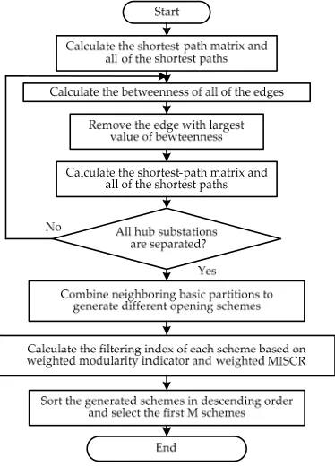
For the parallel loop opening issues, the situation that a lower-voltage isolated power grid partition is separated from the main grid should be avoided. Thus, the power substations in higher voltage power grid are usually selected as hub substations. And each power grid partition consists of at least one hub substation. The maximum possible number of partitions is determined by the number of hub substations. The parallel loop opening process should be stopped when all hub substations are divided into different partitions by GN algorithm.

The generated partitions, each of which contains one hub substation, can be defined as basic partitions. Neighboring basic partitions can be combined in different way to generate different parallel loop opening schemes. An actual AC/DC interconnected power grid contains many higher voltage substations, which usually leads to a huge number of candidate opening schemes. It is usually not necessary to evaluate each of these generated schemes using comprehensive evaluation model because of huge computation time. Thus, a filtering strategy is needed.

According to the analysis above, the weighted modularity indicator can be used to filter the generated opening schemes preliminarily in pure AC power grid. But in AC/DC interconnected power grid, where the influence on MISCR of generated opening schemes must be considered, it is obviously not appropriate to filter opening schemes only based on weighted modularity indicator. Thus, a new filtering index is defined as:

1Q 2M,

ξ λ= ′+λ ′ (12)

where λ1 and λ2 is the weighted coefficients, respectively. There exists the relationship λ1+λ2=1. It

should be noted that λ1 and λ2 are normalized values, not the real algebra values. The new filtering

index is applicable to not only AC/DC interconnected power grid, but also pure AC power grid with

λ1=1, λ2=0.

Figure 1. Generation process of parallel loop opening schemes 4. Evaluation for Parallel Loop Opening Schemes

4.1. Comprehensive Evaluation Model

There are many factors should be considered to evaluate the candidate parallel loop opening schemes. The most principal one is the contradictory relationship between system stability and short-circuit current. In this paper, a comprehensive evaluation model is established based on AHP, which can reflect all of the principal factors. The model is shown in Figure 2.

Figure 2. Comprehensive evaluation model for candidate opening schemes The details of this evaluation model are discussed below:

(a) Static security

Static security should be analyzed with the premise that the system is transferred from a steady state before the fault to another steady state after the fault immediately. The transient process during the fault is not considered. Static security is used to examine whether the operation constraints are satisfied after faults. Operation statuses of key components after specified faults, including line overload, transformer overload and bus voltage limit violation, can be used to evaluate the static security. Thus, two indicators are defined, which are shown below:

Static security B1

Transient stability B2

Operation economy B4 Short-circuit current B3

Over load of line or transformer C11

Transient voltage safety margin C21

Transient angle deviation C22

Short circuit current limit violation C31

Power loss C41

Bus voltage limit violation C12

Target Hierarchy

Rule Hierarchy

Indicator Hierarchy

Candidate parallel loop opening schemes

Indicator C11: over load indicator of line or transformer. 2 11 ( P,l( _maxl ) ) ,n m

l m l S C S γ α ω ∈ ∈

=

 

where γ is the set of specified faults; α is the set of key transmission lines and transformers; ωP,l is the

weighted factor; Sl is the power flow of branch l; Slmax is the upper limit of power flow of branch l; n is

a positive integer.

Indicator C12: bus voltage limit violation indicator. sp

2 12 ( U,( lim ) ) ,

n i i i m i m i U U C U γ β ω Δ ∈ ∈ −

=

 

max min sp _, 2 i i i U U

U = + (15)

max min

lim _,

2

i i

i U U

U

Δ = − (16)

where γ is the set of specified faults; β is the set of buses; ωU,i is the weighted factor; Ui is voltage of

bus i; Uimax and Uimin is the upper and lower limit of voltage of bus i; n is a positive integer.

(b) Transient stability

Transient stability considers the ability of system to maintain stable during the transient process from a steady state before the fault to another steady state after the fault. The transient stability of a power system is composed of voltage stability and power angle stability. Voltage stability is mainly determined by load distribution and load characteristics, which can be measured by transient voltage safety margin. Power angle stability is used to evaluate the interaction between generators with long electrical distance, which can be represented by transient angle deviation. These two indicators are defined as below:

Indicator C21: transient voltage safety margin indicator. 22 ( TV,k k m) ,

m k C

γ η

ω ε

∈ ∈

=

 

where γ is the set of specified faults; η is the set of voltage curves of monitored buses; ωTV,k is the

weighted factor; εk is the transient voltage dip acceptable margin of bus voltage curve k.

Indicator C22: transient angle deviation indicator.

21 ,m(max i j m) ,

m C

γ

ω_θ θ θ

∈

=



where γ is the set of specified faults; ωθ,m is the weighted factor; θi and θj is the power angle of two

generators in the transient process of a specified fault, respectively. (c) Short circuit current

Short circuit current should be limited to not exceed the interrupting capacity of electrical equipment, such as circuit breaker. It can be represented by short circuit current limit violation.

Indicator C31: short circuit current limit violation indicator. 2 31 I,i( _maxi ) ,n

i i I C I β ω ∈

=



where β is the set of buses; ωI,i is the weighted factor; Ii is actual short circuit current of bus i; Iimax is

the maximum interrupting current of circuit breaker of bus i; n is a positive integer. (d) Operation economy

In this paper, power loss is used to represent the operation economy. Indicator C41: power loss indicator.

41 Gen Load,

C =





4.2. Fuzzy Evaluation Algorithm

The comprehensive evaluation model founded above considers almost all of the important factors to evaluate candidate opening schemes. A powerful evaluation algorithm, however, is still needed to find the optimal opening scheme based on the founded model.

Fuzzy evaluation algorithm is based on AHP and fuzzy mathematics [26], which not only includes engineering experience from experts, but also combines the advantages of qualitative analysis and quantitative calculation. Thus, fuzzy evaluation algorithm could avoid the disadvantage of expert system, including uneasy knowledge representation and long computation time [27], which guarantees an effective and fast way to find the optimal opening scheme.

The priority index P of any parallel loop opening scheme can be obtained by fuzzy evaluation algorithm, and the scheme with the largest priority index in the M-dimensional candidate opening scheme set is selected as the optimal one.

5. Case Study

In this section, New England 39-bus system and an actual AC/DC interconnected power system are used as examples to validate the effectiveness and superiority of proposed method.

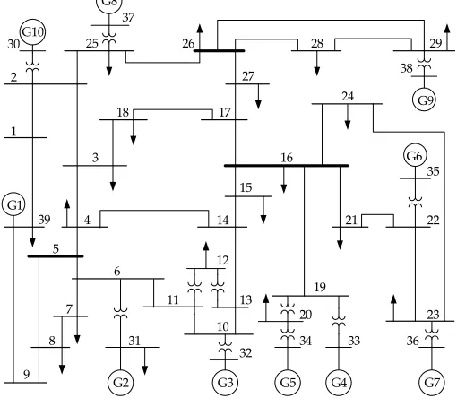
5.1. New England 39-Bus System

New England 39-bus system is a pure AC system, which is shown in Figure 3. Many parallel loops would emerge if a higher voltage power grid is connected to this system via node 5, 16 and 26. With node 5, 16 and 26 as hub substations, this power grid can be divided into three basic partitions at most after switching off several specific lines.

Figure 3. New England 39-bus system

According to the complex network theory in section 2, edge betweenness of each branch should be calculated before switching off any line. The calculation results are shown in Table 1.

Table 1. Edge Betweenness of Each Branch

Branch Edge Betweenness

First partition Second partition Third partition Forth partition

bus1-bus2 1.2581 1.6293 4.0836 0.3300

bus1-bus39 1.1759 1.9265 4.9039 switched off

G10 30

2

1

39 G1

9 8

5

7 6 4

3 18

G2 31 G8

25 37

17 26

27

16

15

11 12

G3 10

13 14

G7 G6

23

36

21 22

G9

28 29

24

19

G5 20

34

G4 33

35

32

bus2-bus3 1.4398 0.7426 2.0915 0.3789

bus2-bus25 0.6875 0.4990 0.7762 0.1663

bus3-bus4 2.0273 switched off switched off switched off

bus3-bus18 0.7607 0.6539 1.7082 0.3870

bus4-bus5 1.3723 0.9619 0.8849 0.2309

bus4-bus14 1.1245 1.0598 0.6075 0.1680

bus5-bus6 0.1591 0.1382 0.1799 0.0469

bus5-bus8 0.7860 0.8421 1.6057 0.2695

bus6-bus7 0.3135 0.3503 0.6177 0.1475

bus6-bus11 0.2222 0.1975 0.6502 0.1399

bus7-bus8 0.1755 0.2124 0.3832 0.0693

bus8-bus9 0.8730 1.4367 3.3099 0.3637

bus9-bus39 0.9508 1.8014 4.7288 0.2502

bus10-bus11 0.0907 0.1209 0.1857 0.0518

bus10-bus13 0.1555 0.1598 0.0302 0.0302

bus13-bus14 0.5983 0.5678 0.2636 0.0913

bus14-bus15 2.0250 2.8089 switched off switched off

bus15-bus16 0.8499 1.2654 0.2550 0.1511

bus16-bus17 1.6069 2.3926 2.6247 1.2498

bus16-bus19 0.5283 0.5283 0.5283 0.3131

bus16-bus21 0.6627 0.6627 0.6627 0.3651

bus16-bus24 0.2895 0.2895 0.2895 0.1595

bus17-bus18 0.4444 0.4938 1.0287 0.3045

bus17-bus27 1.0930 1.3706 0.7807 0.7807

bus21-bus22 0.3646 0.3646 0.3646 0.2103

bus22-bus23 0.0289 0.0289 0.0289 0.0289

bus23-bus24 0.9118 0.9118 0.9118 0.5260

bus25-bus26 1.8826 1.5904 2.1747 0.7465

bus26-bus27 0.7679 1.0337 0.7679 0.6054

bus26-bus28 1.2375 1.2375 1.2375 0.7139

bus26-bus29 1.6317 1.6317 1.6317 0.9414

bus28-bus29 0.0152 0.0152 0.0152 0.0152

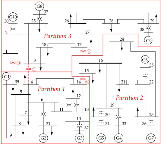
In the original power grid network, the maximum edge betweenness is 2.0273 of line 3-4, which is between bus 3 and bus 4. According to GN algorithm, line 3-4 should be switched off firstly. No new partition emerges after line 3-4 is switched off. Then, the edge bewteennnesses of the modified network without the line 3-4 are calculated. The calculation results are shown in Table 1, too. In this round, the maximum edge betweenness is 2.8089 of line 14-15. No new partition emerges after line 14-15 switched off. During the third round, line 1-39 has the largest edge betweenness, with a value of 4.9039. After line 1-39 switched off, the original network would be divided into two partitions. Since there are still two hub substations in the same partition, the line switching process should be continued until all of the hub substations are divided into different partitions. It should be noted that the edge betweenness of some specific branches in subsequent line switching process might be larger than their corresponding values in previous process, which is due to the change of network connectivity and the branch number along with the line switching process.

Figure 4. Basic partitions of New England 39-bus system

There are three basic partitions illustrated in Figure 4, which can be combined to generate four different opening schemes in total according to Combinatorics and actual neighboring relationship. Because the number of generated opening schemes is quite small, it is not necessary to filter them using the filtering index. The filtering index (Only weighted modularity indicator is considered in this example with λ2 =0.) and priority index of these four generated opening schemes (No.1~4) as

well as two experiential schemes (No.5~6) are shown in Table 2.

Table 2. Filtering Index and Priority Index of Candidate Schemes

No. Candidate Opening Scheme ξ P

1 Partition 1, Partition 2, Partition 3 0.5775 0.5304 2 Partition 1, Partition 2+ Partition 3 0.5327 0.5102 3 Partition 1+ Partition 2, Partition 3 0.5101 0.4854 4 Partition 1+Partition 3, Partition 2 0.5091 0.4603 5 Open line 2-25, line 14-15 and line 3-18 0.4566 0.4517 6 Open line 1-2, line 3-4, line 14-15 and line 16-17 0.4891 0.4633

It is obvious in Table 2 that the filtering index and priority index of first four opening schemes generated by proposed method are overall larger than two experiential schemes. For New England 39-bus system, which is a pure AC power system, a larger filtering index indicates a better network structure after specific lines switched off. And a larger priority index indicates better operation characteristics if the opening scheme is employed. By comprehensively considering the filtering index and priority index, scheme 1 should be selected as the optimal opening scheme. Based on the analysis above, it is easy to recognize the effectiveness of the proposed method to find optimal opening scheme, as well as its superiority over experiential method. The simulation results show that the proposed opening method can successfully be applied in pure AC power system.

5.2. Actual AC/DC Interconnected Power System

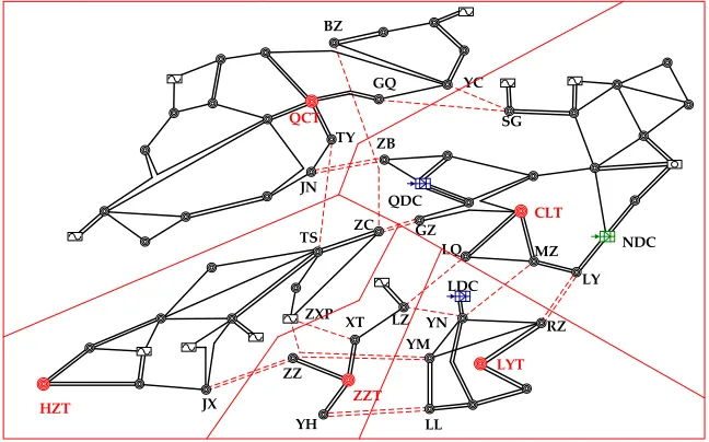
In many modern power systems with intensive load, the AC power system and DC transmission systems are usually operating together and interacting in a complicated way. An actual AC/DC interconnected power system is shown in Figure 5. With the development of 1000kV

G10 30

2

1

39 G1

9 8

5

7 6 4

3 18

G2 31 G8

25 37

17 26

27

16

15

11 12

G3 10

13 14

G7 G6

23

36

21 22

G9

28 29

24

19

G5 20

34

G4 33

35

32

38 Partition 3

Partition 2

③ ①

④

②

transmission systems, 1000kV/500kV parallel loops would emerge, which can be recognized in Figure 5.

Figure 5. Actual AC/DC interconnected power system

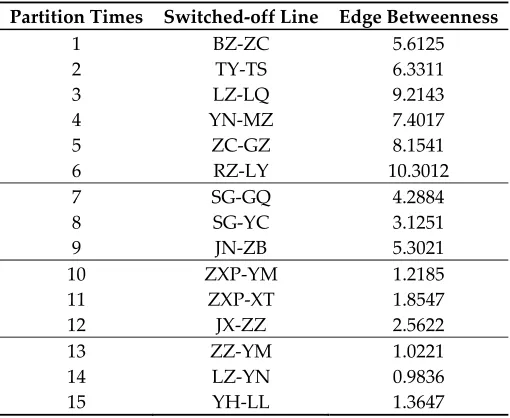
Substation QCT, CLT, LYT, ZZT and HZT are 1000 kV substations, which are also hub substations in this power grid network. The number of hub substations decides the number of basic partitions. Thus, the power grid network can be divided into five basic partitions at most. During the line switching process, the edge betweenness of each branch is dynamically calculated until all of the five basic partitions are separated. Because of the huge amount of branches, it is not appropriate to list the edge betweenness of all of the branches at each line switching round. The switched-off branches and their edge betweenness are shown in Table 3.

Table 3. Computation Results of Edge Betweenness Partition Times Switched-off Line Edge Betweenness

1 BZ-ZC 5.6125

2 TY-TS 6.3311 3 LZ-LQ 9.2143

4 YN-MZ 7.4017

5 ZC-GZ 8.1541

6 RZ-LY 10.3012

7 SG-GQ 4.2884 8 SG-YC 3.1251

9 JN-ZB 5.3021

10 ZXP-YM 1.2185

11 ZXP-XT 1.8547

12 JX-ZZ 2.5622 13 ZZ-YM 1.0221 14 LZ-YN 0.9836

15 YH-LL 1.3647

In this AC/DC interconnected power system, there are three inverter stations: QDC, NDC and LDC. It should be noted that the inverter stations QDC and LDC are hierarchically interconnected to the receiving-end power grid[28]. Thus, each of them is equivalent to two inverter stations (One is in 1000kV power grid and another is in 500kV power grid), respectively. The MISCR calculation results are shown in Table 4. QDC-L and LDC-L are equivalent inverter stations in 500kV power grid. QDC-H and LDC-H are equivalent inverter stations in 1000kV power grid.

BZ

GQ YC

SG TY _ZB

JN

TS ZC GZ

ZXP

JX

ZZ

YH

XT LZ

LQ MZ

LY

YN _RZ

YM

LL

1000kV substation

±800kV Converter station

Thermal plant Nuclear plant 500kV substation

1000kV transmission line 500kV transmission line ±660kV Converter station

QCT

CLT

LYT

ZZT HZT

QDC

NDC

Table 4. MISCR of Each Inverter Station before Optimization

Inverter station MISCR

QDC-L 3.39 QDC-H 3.88 LDC-L 3.40

LDC-H 3.84

NDC 4.32

The basic partitions of this actual power system are shown in Figure 6. After six branches are switched off, the power system is divided into two partitions. And three partitions would emerge with nine branches switched off. Then, there are four partitions with twelve switched-off branches and five partitions with fifteen switched-off branches. These five partitions are basic partitions and can be combined to generate different opening schemes.

Figure 6. Basic partitions of actual power system

According to Combinatorics and the neighboring relationships among basic partitions, 46 different opening schemes can be generated. It is not necessary to have all of these opening schemes evaluated by the comprehensive evaluation model and fuzzy evaluation algorithm, which usually costs a lot of computation time. Thus, the generated opening schemes should be filtered first using the filtering index defined in (11) in section 3. The weighted factors of filtering index are assigned as

λ1=0.5, λ2=0.5. Four generated opening schemes (No.1~No.4) with the largest filtering index as well

as two experiential opening schemes (No.5~No.6) are selected as the candidate opening schemes, whose filtering indices and priority indices are shown in Table 5. In addition, the original network with no branch being switched off acts as the control group (No. 7) to highlight the effect of optimal opening scheme.

Table 5. Filtering Index and Priority Index of Candidate Schemes

No. Candidate Opening Scheme Q’ M’ ξ P

1 QCT+CLT, LYT+ZZT+HZT 0.6306 0.7681 0.69935 0.5698

2 QCT, CLT, LYT+ZZT+HZT 0.6507 0.6528 0.65175 0.5417

3 QCT+HZT+ZZT, CLT+ LYT 0.5291 0.6823 0.6057 0.5206

4 QCT+HZT, CLT+ LYT +ZZT 0.5213 0.7214 0.62135 0.5257

5 Open lines of YC-SG, GQ-SG, JN-ZB, ZC-GZ,

XT-LZ, ZXP-YM, ZZ-YM, YH-LL 0.5118 0.6924 0.6021 0.4798

BZ

GQ YC

SG

TY _ZB

JN

TS ZC GZ

ZXP

JX

ZZ

YH

XT LZ

LQ MZ

LY

YN _RZ

YM

LL

QCT

CLT

LYT

ZZT HZT

QDC

NDC

6 Open lines of TY-TS, TS-ZC, ZC-ZXP, LZ-LQ,

YN-MZ, RZ-LY 0.4987 0.7422 0.62045 0.5175

7 Original Network 0.4533 0.7825 0.6179 0.5023

In Table 5, the filtering index and priority index of first four opening schemes generated by proposed method are overall larger than two experiential schemes and original network. Based on the analysis above and results in Table 5, it can be concluded that the proposed parallel loop opening method can effectively find optimal opening schemes in AC/DC interconnected power system, which is usually more effective than the method based on engineering experience. Additionally, the comparison between scheme 6 and scheme 7 indicates that the experiential method cannot always guarantee a better opening scheme. According to the priority index in Table 5, scheme 1 should be the optimal opening scheme, with the original network divided into two partitions.

As an AC/DC interconnected power system, the system stability (evaluated by MISCR) should be checked after any opening scheme is employed. The MISCR calculation results after scheme 1 employed are shown in Table 6.

Table 6. MISCR of Each Inverter Station with the Optimal Scheme

Inverter station MISCR

QDC-L 3.50

QDC-H 3.90

LDC-L 3.61 LDC-H 3.88

NDC 4.30

Compared with the MISCR results in Table 4, it can be concluded from Table 6 that system stability is high enough after scheme 1 is employed. From the perspective of time-domain simulation, transient voltage curves of inverter buses of QDC and LDC inverter stations also validate the conclusion, which are shown in Figure 7. After the optimal scheme is employed, the voltage curves of all of four inverter buses are able to recover to stable state faster, which indicates a more stable power system.

Figure 7. Transient voltage curves of inverter buses: (a) QDC-L; (b) QDC-H; (c) LDC-L; (d) LDC-H. Note: Green curves and blue curves are the results before and after the optimal scheme employed, respectively.

The derived optimal scheme has good parallel loop opening effect and strong support ability for multiple HVDC links.

6. Conclusions

With the development of higher voltage power grid, the high and low voltage parallel loops are emerging, which lead to energy losses, even threaten the security and stability of power system. To solve this problem not only in pure AC power gird but also in AC/DC interconnected power grid, a decision optimization method is proposed. With this method, parallel loop opening schemes are generated firstly and evaluated secondly. According to simulation results, this proposed method can be used to find the optimal opening scheme in pure AC power system, which is based on complex network theory and has obvious superiority over experiential method. In addition, this method can be employed in AC/DC interconnected power system successfully. The derived optimal scheme can effectively coordinate the relationship between parallel loop opening effect and support ability for multiple HVDC links.

Acknowledgments: This work was supported by State Grid Corporation of China, Major Projects under Grant SGCC-MPLG020-2012 and SGSDDK00KJJS1600149.

Author Contributions: Dong Yang conceived and proposed the method; Kang Zhao and Hao Tian performed the simulations and analyzed the data; Yutian Liu contributed academic idea and paper framework; Dong Yang and Kang Zhao wrote the paper.

Conflicts of Interest: The authors declare no conflict of interest. References

1. Miller, J.; Balmat, B. Operating problems with parallel flows. IEEE Transactions on Power Systems 1991, 6, 1024-1034.

2. Huang, D.; Shu, Y.; Ruan, J.; Hu, Y. Ultra high voltage transmission in china: Developments, current

status and future prospects. Proceedings of the IEEE 2009, 97, 555-583.

3. Liu, Y.; Fan, R.; Terzija, V. Power system restoration: A literature review from 2006 to 2016. J. Mod.

Power Syst. Clean Energy 2016, 4, 332-341.

4. Granelli, G.; Montagna, M.; Zanellini, F.; Bresesti, P.; Vailati, R. A genetic algorithm-based procedure

to optimize system topology against parallel flows. IEEE Transactions on Power Systems 2006, 21, 333-340.

5. Makela, O.; Warrington, J.; Morari, M.; Andersson, G. In Optimal transmission line switching for

large-scale power systems using the alternating direction method of multipliers, 2014 Power Systems

Computation Conference, 2014.

6. Hou, L.R.; Chiang, H.D. In Toward online line switching method for reducing transmission loss in power

systems, Power and Energy Society General Meeting (PESGM), 2016, 2016; IEEE: pp 1-5.

7. Zhao, L.; Zeng, B. Vulnerability analysis of power grids with line switching. IEEE Transactions on Power

Systems 2013, 28, 2727-2736.

8. Fuller, J.D.; Ramasra, R.; Cha, A. Fast heuristics for transmission-line switching. IEEE Transactions on

Power Systems 2012, 27, 1377-1386.

9. Li, M.; Luh, P.B.; Michel, L.D.; Zhao, Q.; Luo, X. Corrective line switching with security constraints for

the base and contingency cases. IEEE Transactions on Power Systems 2012, 27, 125-133.

10. Wu, J.; Cheung, K.W. In On selection of transmission line candidates for optimal transmission switching in

11. Bacher, R.; Glavitsch, H. Network topology optimization with security constraints. IEEE Transactions

on Power Systems 1986, 1, 103-111.

12. Bacher, R.; Glavitsch, H. Loss reduction by network switching. IEEE Transactions on Power Systems

1988, 3, 447-454.

13. Shao, W.; Vittal, V. In A new algorithm for relieving overloads and voltage violations by transmission line and

bus-bar switching, Power Systems Conference and Exposition, 2004. IEEE PES, 2004; IEEE: pp 322-327.

14. Arya L D; Choube S C; P., K.D. Line switching for alleviating overloads under line outage condition

taking bus voltage limits into account. Electric Power and Energy Systems 2000, 22, 213-221.

15. Chen, L.; Tozyo, H.; Tada, Y.; Okamoto, H.; Tanabe, R. In Reconfiguration of transmission systems with

transient stability constraints, Power Engineering Society Winter Meeting, 2000. IEEE, 2000; IEEE: pp

1320-1324.

16. Zhang, N.; Ye, H.; Liu, Y. Decision support for choosing optimal electromagnetic loop circuit opening

scheme based on analytic hierarchy process and multi-level fuzzy comprehensive evaluation.

Engineering intelligent systems for electrical engineering and communications 2008, 16, 183-191.

17. Yang, D.; Zhao, K.; Liu, Y. Coordinated optimization for controlling short circuit current and

multi-infeed dc interaction. J. Mod. Power Syst. Clean Energy 2014, 2, 374-384.

18. Cormen, T.H.; Leiserson, C.E.; Rivest, R.L.; Stein, C. Introduction to algorithms. MIT press: 2009.

19. Girvan, M.; Newman, M.E.J. Community structure in social and biological networks. Proceedings of the

National Academy of Sciences of the United States of America 2002, 99, 7821-7826.

20. Newman, M.E.J.; Girvan, M. Finding and evaluating community structure in networks. Physical review.

E, Statistical, nonlinear, and soft matter physics 2004, 69.

21. Santo, F.; Marc, B. Resolution limit in community detection. Proceedings of the National Academy of

Sciences of the United States of America 2007, 104, 36-41.

22. Aaron, C.; J., N.M.E.; Cristopher, M. Finding community structure in very large networks. Physical

review. E, Statistical, nonlinear, and soft matter physics 2004, 70.

23. Newman, M.E.J. Analysis of weighted networks. Physical review. E, Statistical, nonlinear, and soft matter

physics 2004, 70.

24. CIGRE. Systems with multiple dc infeed; Paris, 2008.

25. Lin, W.; Tang, Y.; Bu, G.; Shao, Y. In Voltage stability analysis of multi-infeed ac/dc power system based on

multi-infeed short circuit ratio, Power System Technology (POWERCON), 2010 International Conference

on, 2010; IEEE: pp 1-6.

26. Zhang, W.; Liu, Y. Multi-objective reactive power and voltage control based on fuzzy optimization

strategy and fuzzy adaptive particle swarm. International Journal of Electrical Power & Energy Systems

2008, 30, 525-532.

27. Liang, Z.; Yang, K.; Sun, Y.; Yuan, J.; Zhang, H.; Zhang, Z. Decision support for choice optimal power

generation projects: Fuzzy comprehensive evaluation model based on the electricity market. Energy

Policy 2006, 34, 3359-3364.

28. Liu, Z. Global energy interconnection. Academic Press: 2015.