R E S E A R C H
Open Access
Double regularized matrix factorization for
image classification and clustering
Wei Zhou
1*, Chengdong Wu
2, Jianzhong Wang
3,4, Xiaosheng Yu
2and Yugen Yi
5Abstract
Feature selection, which aims to select an optimal feature subset to avoid the “curse of dimensionality,” is an important research topic in many real-world applications. To select informative features from a high-dimensional dataset, we propose a novel unsupervised feature selection algorithm called Double Regularized Matrix Factorization Feature Selection (DRMFFS) in this paper. DRMFFS is based on the feature selection framework of matrix factorization, but extends this framework by introducing double regularizations (i.e., graph regularization and inner product regularization). There are three major contributions to our approach. First, for the sake of preserving the useful underlying geometric structure information of the feature space of the data, we introduce the graph regularization to guide the learning of the feature selection matrix, making it more effective. Second, in order to take into account the correlations among features, an inner product regularization term is imposed on the objective function of matrix factorization. Therefore, the selected features by DRMFFS cannot only represent the original high-dimensional data well but also contain low redundancy. Third, we design an efficient iteratively update algorithm to solve our approach and also prove its convergence. Experiments on six benchmark databases demonstrate that the proposed approach outperforms the state-of-the-art approaches in terms of both the classification and clustering performance.
Keywords: Unsupervised feature selection, Matrix factorization, Feature manifold structure, Sparse and low redundancy
1 Introduction
The dimensionality of the gathered data has been increasingly large due to the rapid development
of modern sensing systems [1]. However, the
high-dimensional data are hard to deal with since
high computational complexity and memory
requirements. Meanwhile, some irrelevant, redundant,
and noisy features will be incorporated into
high-dimensional data, which will adversely affect the performance. Hence, reducing the dimension of the data is an essential step for subsequent processing. Feature extraction [2, 3] and feature selection [4] can be regarded as two main techniques for dimensional-ity reduction. For feature extraction approaches, they obtain the features by mapping the original data
into a new low-dimensional subspace using a
transformation matrix or projection. Nevertheless, the obtained features have relatively poor interpretability
[3]. In comparison, feature selection approaches aim
at selecting several optimal features from the original data by a series of criteria [5]. Therefore, the obtained
low-dimensional representation is interpretable [4].
More importantly, feature selection approaches just need to collect these optimal features during data ac-quisition, and they perform better than feature extrac-tion approaches, which need to utilize all the features for dimensionality reduction. In this paper, we focus on feature selection.
Many feature selection approaches have been pro-posed in recent years. According to the availability of class label information, they can be categorized into three classes, including supervised feature selection [6], semi-supervised feature selection [7], and unsupervised feature selection [8, 9]. Supervised-based feature selec-tion approaches search the optimal feature subset with the guidance of the class label information. However, in
* Correspondence:[email protected]
1College of Information Science and Engineering, Northeastern University,
Shenyang 110819, China
Full list of author information is available at the end of the article
many real applications, there are small amount of la-beled data or labeling all the data requires quite expen-sive human labor and computational costs. Therefore, supervised-based feature selection approaches are not feasible in the case of partially labeled data. Under this circumstance, a series of semi-supervised feature selec-tion approaches have been designed, which take the in-formation of the labeled and unlabeled data into account. Compared with the aforementioned feature se-lection techniques, unsupervised feature sese-lection ap-proaches determine an optimal feature subset, without any label information, and only depend on maintaining or revealing the intrinsic structures of the original data. Hence, how to incorporate the intrinsic structure infor-mation of the data into unsupervised feature selection is very critical.
A series of unsupervised feature selection approaches have been proposed. Among them, Variance Score (VS) might be the simplest unsupervised feature selection al-gorithm [10], which selects features based on their
vari-ance. After that, He et al. took advantage of
locality-preservation ability of features and proposed an unsupervised feature selection approach called Laplacian
Score (LS) [11]. The features selected by LS can
main-tain the manifold structure of the original data. In the sequel, Zhao and Liu combined the spectral graph the-ory into feature selection and presented Spectral Feature Selection (SPEC) [12]. In essence, VS, LS, and SPEC esti-mate the quality of features independently, ignoring the correlation among features.
In order to address the aforementioned issue, a series of sparsity regularization-based approaches have been presented [8, 9, 13–23] for unsupervised feature
selection. For instance, Cai et al. presented
Multi-Cluster Feature Selection (MCFS) [8] by
com-bining spectral analysis (manifold learning) and sparse
regression based on l1-norm regularization. In MCFS,
spectral analysis and sparse regression are two inde-pendent processes, and thereby, the effectiveness is degraded. To address such limitation, a series of stud-ies which simultaneously perform the spectral analysis and sparse regression have been presented for
un-supervised feature selection [9, 13–23]. Yang et al.
proposed Unsupervised Discriminative Feature
Selec-tion (UDFS) [9] to select the most discriminative
fea-tures for data representation. Similar to UDFS, Cong et al. proposed Unsupervised Deep Sparse Feature
Se-lection (UDSFS) [13], which integrates the group
sparsity of feature dimensions and feature units based
on an l2, 1-norm minimization into a unified
frame-work to select the most discriminative features. Li et al. presented Nonnegative Discriminative Feature
Se-lection (NDFS) [14], which performs non-negative
spectral analysis and feature selection together. Yang
et al. suggested Unsupervised Maximum Margin
Fea-ture Selection (UMMFSSC) [15]. In UMMFSSC, the
clustering process and feature selection process are combined into a coherent framework to adaptively se-lect the most discriminative subspace. Since the data always contain noise or outliers, Qian et al. proposed
Robust Unsupervised Feature Selection (RUFS) [16] to
address it, where robust clustering and robust feature
selection are simultaneously performed by joint l2,
1-norm minimization. Recently, self-representation property has been extensively utilized and many
re-lated approaches have been proposed [17]. In [18],
Zhu et al. assumed that each feature can be repre-sented as a linear combination of other features and proposed Regularized Self-Representation (RSR). Al-though good performance can be achieved by RSR, the structure preserving ability of features is neglected in it. To remedy it, a variety of extensions based on RSR have been put forward, i.e., Graph Regularized
Nonnegative Self-Representation (GRNSR) [19] and
Structure Preserving Nonnegative Feature
Self-Representation (SPNFSR) [20]. Besides, Zhu et al.
combined manifold learning and sparse regression to-gether and proposed Joint Graph Sparse Coding
(JGSC) [21]. In JGSC, a dictionary is firstly learned
from the training data; then, the feature weight matrix can be obtained automatically via the learned dictionary. Since real-world data always contain lots of noise samples and features, the learned dictionary may be unrealizable to subsequent feature selection
process [22]. Different from most of the
aforemen-tioned approaches which only utilize the geometric information of the data space, Shang et al. employed the manifold information of both the data space and
the feature space simultaneously and proposed
Non-Negative Spectral Learning with Sparse
Regression-Based Dual-graph regularized feature
se-lection (NSSRD) [23]. Through the experimental
re-sults in [23], it can be seen that the geometry
information of the feature space plays a crucial role for further improving the quality of feature selection.
Apart from the above sparsity regularization-based un-supervised feature selection approaches, a series of matrix factorization-based approaches have been pre-sented. Well-known examples of such methods include
Principal Components Analysis (PCA) [24],
Non-negative Matrix Factorization (NMF) [25], and
Sin-gular Value Decomposition (SVD) [26]. Nevertheless,
these approaches are all designed for feature extraction
rather than feature selection. Therefore, the
approach named Matrix Factorization based Feature Se-lection (MFFS) [27]. In MFFS, the feature selection can be regarded as the process of matrix factorization and the optimal feature subset is selected by introducing an orthogonality constraint into its objective function. Con-sidering that MFFS conducts feature selection by inte-grating matrix factorization with an orthogonality constraint together, the orthogonality constraint is too strict to be satisfied in practice [23,28,29].
As previously mentioned, there are mainly two issues to these approaches. On the one hand, most of the
state-of-the-art unsupervised feature selection
ap-proaches (e.g., LS, SPEC, MCFS, UDFS, UDSFS, NDFS, UMMFSSC, RUFS, GRNSR, SPNFSR, JGSC) can only take the geometric and discrimination information of the data space into consideration, while neglecting the useful underlying geometric structure information of the feature space during the process of dimensionality re-duction [23]. Hence, some potentially valuable informa-tion is not fully exploited, reducing the performance of the algorithm. On the other hand, the majority of the existing approaches (e.g., MCFS, UDFS, UDSFS, NDFS, UMMFSSC, RUFS, RSR, GRNSR, SPNFSR, JGSC, and
NSSRD) impose thel1-norm regularization orl2, 1-norm
regularization on the feature weight matrix aiming to perform feature selection in a batch manner.
Neverthe-less, the l1-norm or l2, 1-norm neglect the redundancy
measurement, so methods using l1-norm regularization
orl2, 1-norm regularization might get into trouble when dealing with some informative but redundant features [30]. In general, the use of the l1-norm or l2, 1-norm regularization cannot achieve both sparsity and low re-dundancy simultaneously.
To address the above issues, this paper presents a novel approach called Double Regularized Matrix Factorization Feature Selection (DRMFFS) for conduct-ing classification and clusterconduct-ing on high-dimensional data. Compared with the existing feature selection ap-proaches, our main contributions lie in the following three-fold. First, to preserve the manifold information of the feature space, graph regularization which is a feature map constructed on the feature space, is imposed on the feature selection framework of matrix factorization. With the use of it, the learning of the coefficient matrix in error reconstruction term and the feature selection matrix can be guided. Therefore, it cannot only select a feature subset that can approximately represent the fea-tures, but also preserve the local geometrical informa-tion of the feature space. Second, to ensure the sparsity and low redundancy simultaneously, we introduce an inner product regularization term that can be regarded
as a combination of thel1-norm andl2-norm on the
ob-jective function of matrix factorization. Third, a simple yet effective iteration update algorithm is proposed to
optimize our model and a detailed analysis of its conver-gence is also given. Experiments on six databases, in-cluding Extended YaleB [31], CMU PIE [32], AR [33],
JAFFE [34], ORL [35], and COIL20 [36] demonstrate
that the proposed approach is effective.
The rest of this article is organized as follows: Section
2 presents the proposed method in detail. The
experi-mental results and discussion are shown in Section3. In the end, the conclusions are given in Section4.
2 Methods
Firstly, the proposed DRMFFS model is given in detail. Secondly, we design an efficient iterative update algo-rithm to solve our model. Thirdly, we analyze its conver-gence. Finally, we compare the proposed approach with the related approaches to demonstrate its effectiveness.
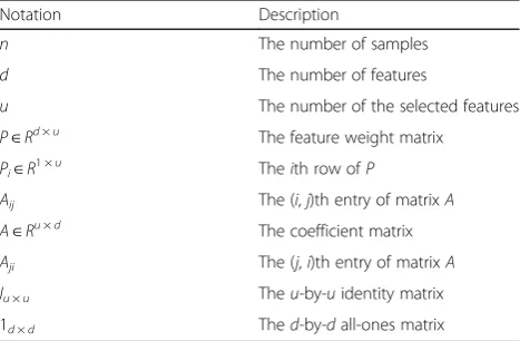
Table 1 gives some notation that is frequently used in
this paper, which aims to facilitate the presentation.
2.1 The DRMFFS model
LetX= [x1;x2;…;xn]∈Rn×dbe the high-dimensional
un-labeled input data matrix, where n and d, respectively,
represent the number and dimension of samples. The proposed approach aims to select a handful of optimal features that can approximately represent the entire set of features. Therefore, the distance between the spaces spanned by the original high-dimensional data samples and the selected features can be evaluated. According to
[27], this problem can be converted into the following
matrix factorization problem:
arg min
P;A kX−XPAk 2
F
s:t: P≥0;A≥0;PTP¼Iuu; ð
1Þ
where A= [a1,a2,…,ad]∈R u×d
is the coefficient
matrix used to project the original features into a new feature subspace spanned by the selected features,Iu×uis the u×u identity matrix, P= [p1,p2,p3,…,pd]
T∈
Rd×u
denotes the feature weight matrix, and u denotes the
Table 1Some notation used in the paper Notation Description
n The number of samples
d The number of features
u The number of the selected features
P∈Rd×u The feature weight matrix
Pi∈R
1 ×u
Theith row ofP
Aij The (i,j)th entry of matrixA
A∈Ru×d The coefficient matrix
Aji The (j,i)th entry of matrixA
Iu×u Theu-by-uidentity matrix
count of the selected features. The constraintPTP=Iu×u
is used to ensure that the elements in P are ones or
zeros. Here, we regard the matrix P as an indicator
matrix of the selected features.
Although Eq. (1) can accomplish the feature
selec-tion task, there remain two drawbacks. First, the underlying geometric information of the feature space is neglected, which weakens the quality of feature se-lection. Second, the orthogonality constraint in Eq. (1) is too strict [23], which ignores the correlations among features.
Actually, local structure information plays an im-portant role in feature selection. Therefore, many
fea-ture selection algorithms using local structure
information have been proposed and achieve good
performance. For example, Laplacian Score (LS) [11],
Spectral Feature Selection (SPEC) [12], and
Multi-Cluster Feature Selection (MCFS) [8] are three
well-known algorithms. Meanwhile, some researchers have shown that the manifold information of the data is distributed not only in the data space but also in
the feature space [37–40]. Therefore, the feature
manifold also contains the underlying geometric
structure information, which is beneficial for feature
selection. Inspired by [37–40], we incorporate the
local structure information of the feature space of the data into our algorithm to address the first
shortcom-ing of Eq. (1). First, we build a k-nearest neighbor
graph G= (V,E) based on the given sample matrix X.
Here, each row vector of X corresponds to a feature,
i.e., fjis the jth feature of X. Then, we can rewrite X asX= [f1;f2;…;fd]∈R
d×n
. For a graph G, we denote
the set of feature points and the weights of the edges between the vertices, as V= [f1,f2,…,fd] and E= [E1,
E2,…,Ed], respectively. Specifically, we can regard the weight of the edge as the similarity between the two features, namely, the higher the weight, the more similar the features.
To ensure that the selected features retain the
geom-etry information of the features in the original
high-dimensional feature space, we can minimize the following equation:
J ¼ arg min A 1 2 Xd i¼1 Xd j¼1
ai−aj
2
2Sij ð2Þ
where ai is the low-dimensional representation of fi, and Sij represents the similarity between featuresfi and
fj, (i,j= 1, 2,…,d).
Since Gaussian heat kernel function is a simple and effective approach to discover the intrinsic geomet-rical structure of the data [3, 41, 42], this paper uti-lizes it to measure the closeness between features, which is defined as:
Sij¼ exp − fi−fj
2
2=σ 2
; if fi∈N fj orfj∈N fð Þi
0 otherwise;
8 < :
ð3Þ
where N(fi) is the k-nearest neighbor set of feature fi and σis a kernel parameter. If features fiand fjare close in the original high-dimensional feature space, the corre-spondingSijwill be large, and vice versa.
By simple algebraic manipulation, Eq. (2) can be
re-written to:
J¼ arg min A 1 2 Xd i¼1 Xd j¼1
ai−aj
2
2Sij
¼ arg min
A tr A Dð −SÞA T
¼ arg min A tr ALA
T
;
ð4Þ
where D is a diagonal matrix and Dii=∑jSij. The
matrix L=D-S is the graph Laplacian matrix of feature space. According to Eq. (3), it is easy to see that if two features, e.g., fi and fj, are close to each other, then the similarity measurementSijis large. Actually, by minimiz-ing Eq. (4), we tend to find such a matrixAthat ensures that if the nearby features, e.g., fi and fj, are related to each other, and their corresponding low-dimensional representations, i.e.,aiand aj, should still have the same and similar relations.
The second shortcoming of Eq. (1) is the strict orthog-onality constraint. A straightforward way to address it is to introduce the existing regularization terms, such as the l1-norm or l2, 1-norm with respect to P in Eq. (1). Nevertheless, the characteristics of sparsity and low
re-dundancy could not be achieved simultaneously [37] by
these regularization terms. Recently, Han et al. designed a regularization term that can directly characterize the independence and saliency of variables [37]. Inspired by [37], in this paper, we utilize the absolute values of the inner product between feature weight vectors as the regularization term to relax the strict orthogonality con-straint of Eq. (1), i.e.,∣<pi,pj>∣, in whichpj∈R1 ×u(j= 1, 2,…,d) is thejth row vector of P. Therefore, we can rewrite the regularization in our DRMFFS as:
Ωð Þ ¼P X
d
i¼1 Xd
j¼1;j≠i
j<pi;pj>j
¼Xd
i¼1 Xd
j¼1
j<pi;pj>j− Xd
i¼1
j<pi;pi>j
¼X
d
i¼1 Xd
j¼1
j<pi;pj>j−X
d
i¼1
pi
k k2 2:
ð5Þ
Ωð Þ ¼P PPT 1−tr P TP
¼ PPT 1−k kP 22
: ð6Þ
Finally, we expect the metric in Eq. (6) to be as small as possible [37], and the weights that correspond to the redundant and uninformative features will be reduced to very small values or even zeros, which makes the feature selection more discriminative.
Next, through combining Eqs. (4) and (6) with the
matrix factorization, the objective function of our DRMFFS algorithm can be obtained as:
min
P;A kX−XPAk
2
Fþαtr ALA T
þβΩð ÞP
¼ min
P;A kX−XPAk
2
Fþαtr ALAT
þβX d
i¼1
Xd
j¼1;j≠i
j<pi;pj>js:t: P≥0; A≥0;
ð7Þ
whereα≥0 andβ≥0 are two balance parameters. The
first term measures the ability of the selected features; the second term aims at ensuring that the selected fea-tures can maintain the geometry structure information of the features in the original high-dimensional feature space; the third term is used to make the feature weight matrix sparse and of low redundancy.
By optimizing the proposed objective function, the fea-ture weight matrix P= [p1;p2;…;pd] can be learned. Then, we can rank all the features in terms of ‖pi‖2 in
descending order and select the first ufeatures to form
the optimal feature subset.
2.2 Iterative updating algorithm
In Eq. (7), it contains two variables, i.e., P and A. Con-sidering that Eq. (7) is not convex, we give an iterative update algorithm to optimize Eq. (7).
LetF(P,A) be the value of the objective function of Eq. (7), that is,
F Pð ;AÞ ¼kX−XPAk2Fþαtr ALA T
þβXd i¼1
Xd
j¼1;j≠i
j<pi;pj>j¼kX−XPAk
2
F
þαtr ALA Tþβ PPT 1−k kP 22
s:t:
P≥0;A≥0:
ð8Þ
After some algebraic manipulations, we can rewrite Eq. (8) as
F Pð ;AÞ ¼kX−XPAk2Fþαtr ALAT
þβ PPT 1‐k kP 22
¼trðX‐XPAÞTðX‐XPAÞþαtr ALA T þβ tr 1ddPPT
‐tr P TP
¼tr X TX
‐2tr A TPTXTXþtr A TPTXTXPA
þαtr ALA Tþβ tr 1ddPPT
‐tr P TP
; ð9Þ
where 1d×dis a d×d matrix with all the elements
equal to 1.
Next, we introduce two Lagrange multipliers λ∈Rd×
u
and ϑ∈Ru×d to constrain P≥0andA≥0, respectively. So Eq. (9) can be rewritten as Lagrange’s function:
L Fð ;λ;ϑÞ ¼ F Pð ;AÞ þtrð Þ þλP trð ÞϑA
¼tr X TX−2tr A TPTXTX
þtr A TPTXTXPAþαtr ALA Tþβðtr1ddPPT
−tr P TPÞ þtrð Þ þλP trð ÞϑA:
ð10Þ
By taking the derivatives of Eq. (10) with respect to P
andA, and setting them equal to zero, we get:
∂L
∂P¼−2X
TXATþ2XTXPAATþ2βð1ddP−PÞ
þλ
¼0 ð11Þ
∂L
∂A¼−2P
TXTXþ2PTXTXPAþ2αA Dð −SÞ
þϑ
¼0: ð12Þ
Using the Karush-Kuhn-Tucker (KKT) [43] conditions
λijPij= 0 andϑjiAji= 0, we obtain:
Pij←Pij
XTXATþβP
ij
XTXPAATþβ1 ddP
ij
; ð13Þ
Aji←Aji
PTXTXþαAS
ji
PTXTXPAþαAD
ji
: ð14Þ
The whole procedure of our algorithm is summarized in Algorithm 1. First, we need to calculate the similarity matrix among features, whose computation complexity isΟ(d2n). Then, the time complexity of each iteration in Algorithm 1 is equal to Ο(u2d+nd2+ud2). Note that the number of the selected featuresuis smaller than the
number of original features d. So, the total time
2.3 Convergence analysis
The convergence of the update criteria in Eqs. (13) and (14) are given as follows:
2.3.0.1 Theorem 1. ForP≥0,A≥0, the value of the ob-jective function in Eq. (8) is non-increasing and has a
lower boundary under the update rules in Eq. (13) and
Eq. (14).
Here, we incorporate an auxiliary function to prove Theorem 1, which is defined as follows:
2.3.0.2 Definition 1. ϕ(v,v') is an auxiliary function of ψ(v) if conditionsϕ(v,v')≥ψ(v)andϕ(v,v) =ψ(v) are satis-fied [25].
The auxiliary function is very useful because of the fol-lowing lemma:
2.3.0.3 Lemma 1. Suppose that ϕ is an auxiliary func-tion of ψ; then, ψis non-increasing under the following update rule:
vðtþ1Þ¼ arg min v ϕ v;v
t ð Þ
; ð15Þ
wheretindicates thetth iteration.
Proofψ(v(t+ 1))≤ϕ(v(t+ 1),v(t))≤ϕ(v(t),v(t)) =ψ(v(t)).□ First, it is necessary to prove that the update criterion forPin Eq. (13) is consistent with Eq. (15) when an aux-iliary function is properly designed. We defineψij(Pij)as the part of Eq. (8) that is only related toPij. Therefore, we have:
ψij Pij ¼ ð−2ATPTXTXþATPTXTXPA
þβ1ddPPT−βPTPÞij; ð16Þ ∇ψij Pij ¼ ð−2XTXATþ2XTXPAAT
þ2β1ddP−2βPÞij; ð17Þ
∇2ψ
ij Pij ¼2 XTX
ii A TA
jjþ2βð1dd−IÞii; ð18Þ
where ∇ψij(Pij) and ∇2ψij(Pij) represent the first-order and second-order derivatives, respectively, of the object-ive functionψijwith respect toPij.
2.3.0.4 Lemma 2. The function in Eq. (19) is a reason-able auxiliary function ofψij(Pij).
ϕPij;Pð Þijt¼ψijPð Þijt þ∇ψijPð Þijt Pij−Pð Þijt
þ X
TXPAATþβ1 ddP
ij
Pð Þijt Pij−P
t ð Þ ij
2
:
ð19Þ
Proof Through the Taylor series expansion of ψij(Pij), we obtain:
ψij Pij ¼ψij P t ð Þ ij
þ∇ψij P t ð Þ ij
Pij−Pð Þijt
þ1 2∇ 2ψ ij P t ð Þ ij
Pij−Pð Þijt
2
¼ψij P t ð Þ ij
þ∇ψij P t ð Þ ij
Pij−Pð Þijt
þ XTX ii A
TA
jjþβð1dd−IÞii
n o
Pij−Pð Þijt
2
: ð20Þ
Through integrating Eq. (19) with Eq. (20), we can
learn thatϕðPij;PijðtÞÞ≥ψijðPijÞis equivalent to:
XTXPAATþβ1 ddP
ij
Pð Þijt ≥ X
TX ii A TA jj
þβð1dd−IÞii: ð21Þ
In according with linear algebra, we can obtain:
XTXPAAT
ij¼
Xu
l¼1
XTXPð Þt
il A TA
lj≥ X TXPð Þt
ij A TA
jj
≥Xd l¼1
XTX
ilP t ð Þ lj AA T jj
≥XTX iiP
t
ð Þ
ij AAT
jj¼P t
ð Þ
ij XTX
ii AA T
jj:
βð1ddPÞij¼βX
d
l¼1 1dd
ð ÞilP t ð Þ lj ≥β
Xd
l¼1
1dd−I
ð ÞilP
t ð Þ lj
≥βð1dd−IÞiiPð Þijt :
ð23Þ
From Eqs. (22) and (23), we observe that Eq. (21) holds and ϕðPij;PðijtÞÞ≥ψijðPijÞ. In addition, ϕðPij;PðijtÞÞ
¼ψijðPijÞis obvious. Thus, Lemma 2 is proved.□
Next, we employ the similar method as that described above to analyze the variable A. We use ψji(Aji) to de-note the part of Eq. (8) and obtain:
ψji Aji ¼ −2ATPTXTXþATPTXTXPAþ2αALAT
ji
ð24Þ
∇ψji Aji ¼ −2PTXTXþ2PTXTXPAþ2αAL
ji
ð25Þ
∇2ψ
ji Aji ¼2 PTXTXP
jjþð ÞL ii ð26Þ
where∇ψji(Aji) and∇2ψji(Aji) represent the first-order and second-order derivatives ofψjiwith respect toAji.
2.3.0.5 Lemma 3. The following function in Eq. (27) is a reasonable auxiliary function ofψji(Aji).
ϕ Aji;Ajið Þt
¼ψji Ajið Þt
þ∇ψji Ajið Þt
Aji−Ajið Þt
þ P
TXTXPAþAD
ji
Ajið Þt
Aji−Ajið Þt
2
:
ð27Þ
Proof Through the Taylor series expansion of ψji(Aji), we obtain:
ψ Aji ¼ψji Ajið Þt
þ∇ψji Ajið Þt
Aji−Ajið Þt
þ1
2∇ 2ψ
ji Ajið Þt
Aji−Ajið Þt
2
¼ψji Ajið Þt
þ∇ψji Ajið Þt
Aji−Ajið Þt
þ PTXTXP jjþLii
n o
Aji−Ajið Þt
2
:
ð28Þ
Through comparing Eq. (27) with Eq. (28), it is easy to see thatϕ(Aji,Aji(t))≥ψji(Aji)equals to:
PTXTXPAþAD
ji
Ajið Þt
≥PTXTXPjjþLii: ð29Þ
In according with the linear algebra, we obtain:
PTXTXPA
ji¼ Xu
l¼1
PTXTXP
jlA t ð Þ
li ≥ PTXTXP
jjA t ð Þ ji :
ð30Þ
AD
ð Þji¼ Xu
l¼1
Að ÞjltDli≥Að ÞjitDii
¼Að ÞjitDii≥Að Þjit ðDii−SiiÞ ¼Að ÞjitLii: ð31Þ
From Eqs. (30) and (31), we know that Eq. (29) holds and ϕ(Aji,Aji(t))≥ψji(Aji). Considering that we can check
ϕ(Aji,Aji(t)) =ψji(Aji) easily, Lemma 3 is proved.□. Finally, we will give a proof of the convergence of The-orem 1.
Proof of Theorem 1 we use the auxiliary function in
Eq. (19)to replaceϕ(v,v(t))inEq. (15)and obtain:
Pðijtþ1Þ¼Pijð Þt−Pð Þijt ∇ψij Pð Þijt
2XTXPAATþβ1ddPij
¼Pð Þijt X
TXATþβP
ij
XTXPAATþβ1ddP
ij :
ð32Þ
Likewise, we utilize the auxiliary function in Eq. (27) to replaceϕ(v,v(t)) in Eq. (15) and obtain:
Aðjitþ1Þ¼Ajið Þt−Að Þjit ∇ψji Að Þjit
2PTXTXPAþαADji
¼Að Þjit P
TXTXþαAS
ji
PTXTXPAþαAD
ji :
ð33Þ
Since Eqs. (19) and (27) are the auxiliary functions of ψij,ψijis non-increasing under the update criteria in Eqs. (13) and (14). Lastly, considering that all of the terms in Eq. (8) are non-negative, the objective function of the proposed DRMFFS approach has a lower bound. Hence, in accordance with Cauchy’s convergence rule [44], the
proposed model is convergent.□
2.4 Comparison with other approaches
In this subsection, we will highlight the effectiveness of our DRMFFS from the following two aspects:
(1) We compare our DRMFFS with the related
the feature space, which can provide more accurate discrimination information for feature selection. Secondly, for sparsity regularization-based unsupervised feature selection approaches, such as MCFS, UDSFS, RUFS, RSR, SPNFSR, JGSC, and NSSRD, they select a subset of features based on the l1-norm orl2, 1-norm. However, these approaches except UDSFS ignore the correlation among features, and thereby, the features selected by them may contain some redundancy, which makes the feature subset far from optimal. In contrast, our approach employs the absolute values of the inner product of the feature weight matrix vectors as a
regularization term to ensure that the feature subset contains sparsity and low redundancy simultaneously. Finally, in comparison with Matrix Factorization-Based Feature Selection approach, i.e., MFFS, our DRMFFS uses the inner product constraint term in place of the strict orthogonality constraint term making our approach more flexible and effective.
(2) We utilize the visualization of the features selected by different approaches to further demonstrate the effectiveness of our DRMFFS. First, we randomly select three sample images with the size of 32 × 32 pixels from three different face databases, i.e., ORL, AR, and CMU PIE. Then, all the approaches are applied to them and the selected features are labeled on this image. Here, the number of the selected features is fixed as 100 for all of the approaches. Figure1illustrates the corresponding experimental results, in which red color is used to represent the selected features and the features which are not selected retain the original gray. As seen from Fig.1, all of the approaches except our DRMFFS select the features from uninformative parts of the face, such as the forehead and cheek or evenly distributed on the face. On the contrary, our DRMFFS can select the most representative face features, such as the eyes, eyebrows, nose, and mouth. Actually, observing Fig.1, we can find two interesting phenomena as follows. On the one hand, the features selected by DRMFFS mostly focus on the recognizable parts of the face (i.e., eyes, eyebrows, nose, and mouth). The main reason is that our DRMFFS uses the graph regularization to preserve the geometric structure information on the feature manifold, making the selected features more holistic and structural. On the other hand, the selected features which are used to represent the eyes, mouth, and nose are mainly from the one side of the face. This phenomenon is due to the fact that DRMFFS takes the correlations among features into consideration, and thereby, the selected features are
mainly from one side of the nearly symmetrical face components, accomplishing the low-redundancy.
Besides, we randomly select a sample image from Ex-tended YaleB database as the experimental sample and
apply our DRMFFS to this sample. Figure 2 shows the
visualization result of our approach under different number of selected features. In Fig. 2, the red color is used to represent the selected features and the features which are not selected retain the original gray. Here, the number of selected features is tuned from {20, 50, 100,
150, 200, 250, 300}. Seen from Fig. 2, when the number
of selected features is relatively small, the outline of the human face is not clear since the selected features rarely locate on the recognizable parts of the face. However, with the increase in number of selected features (from left to right), the extracted face information is also in-creased. In other words, our DRMFFS fails to select the most representative features such as the mouth and nose when the number of selected features is relatively small. The reason for the degraded performance of our DRMFFS under less number of features is that our ap-proach utilizes the distance between the spaces spanned by the original high-dimensional data samples and the selected features as the evaluation criterion (see Eq. (1)). Therefore, when considering smallest features to be se-lected, the space spanned by our approach cannot well approximate the space spanned by original input sam-ples, which leads to the information of high-dimensional data cannot be sufficiently maintained.
3 Results and discussion
In this section, we will carry out classification and clustering experiments to verify the effectiveness of the
proposed approach in comparison with other
state-of-the-art approaches.
3.1 Database
In our experiment, we use six benchmark image data-bases, including Extended YaleB [31], CMU PIE [32], AR [33], JAFFE [34], ORL [35], and COIL20 [36], to com-pare the performance of our approach with those of the
state-of-the-art unsupervised feature selection
ap-proaches. Detailed descriptions of the six databases are
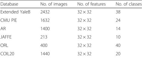
given in Table 2, and some image examples from these
databases are shown in Fig.3.
(2) CMU PIE [32]: it includes 41,368 face images of 68 persons. In our experiment, we choose a subset (C29) that contains 210 face images of 10 persons from this dataset. Example images are shown in Fig.3b.
(3) AR face [33]: it consists of 4000 facial images that depict 126 distinct subjects (70 male and 56 female
faces). The images of each subject were taken in varying conditions. The example images are shown in Fig.3c.
(4) JAFFE [34]: there are 213 facial images in it. Each person has seven different kinds of facial
expressions. The example images from AR are given in Fig.3d.
(a)
(b)
(c)
Fig. 1The visualization results of selected features by different approaches on three different databases.aA sample image coming from ORL.b A sample image coming from AR.cA sample image coming from CMU PIE
(5) ORL [35]: there are ten different images of each of 40 distinct subjects. For each subject, the images were taken at different times, varying the lighting conditions. The example images from ORL are depicted in Fig.3e.
(6) COIL20 [36]: it is a database of gray-scale images of 20 objects. Each of subjects has 72 images, which were taken at pose intervals of 5° to vary object pose with respect to a xed camera. The example images from this database are illustrated in Fig.3f.
3.2 Experimental settings
In our experiments, we choose ten representative un-supervised feature selection algorithms as the compari-son approaches. The ten comparicompari-son approaches include LS [11], MCFS [8], SPEC [12], UDSFS [13], RUFS [16], RSR [18], SPNFSR [20], JGSC [21], NSSRD [23], and
MFFS [27]. Meanwhile, several details for the
experi-ment parameter setting are as follows. For LS, MCFS, SPEC, UDSFS, SPNFSR, JGSC, NSSRD, and our
approach, we fix the number of neighborhoods to 5 on all the databases. For UDSFS, RUFS, RSR, SPNFSR, JGSC, and NSSRD, the sparsity parameters will be tuned by a grid-search strategy from{10−3, 10−2, 10−1, 100, 101, 102, 103}. Following [27], we fix the value of the
param-eter in MFFS to 108. For DRMFFS, we exploit the
pa-rameters α and βin the range of {0, 100, 101, 102, 103, 104, 105} on all the databases. We will report the best re-sults obtained from the optimal parameters for all the approaches.
3.3 Classification results and analysis
In this subsection, we perform six different experiments on three databases including the Extended YaleB, CMU PIE, and AR to verify the effectiveness of our approach.
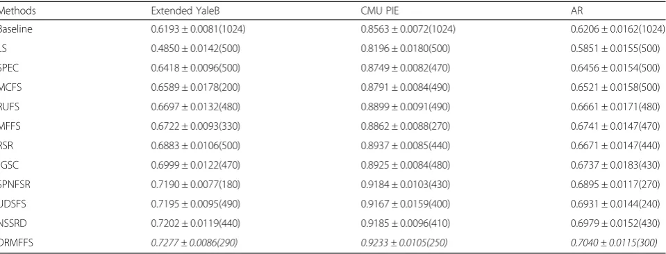
In the first experiment, we choose randomly l (l= 20, 12, 7) images per class for training from each of the three databases and reserve the remaining images for testing. The process is repeated 10 times, and the aver-age classification accuracies and standard deviations of
different approaches are reported in Table 3. Since the
experiment environment and setting are the same with
our previous paper [19]. Hence, a part of experimental
results of the comparison approaches are directly from
our previous work [19]. The number in parentheses is
the number of the selected features that corresponds to the best result. Analyzing Table 3, it is obvious that all the feature selection approaches except LS outperform the baseline approach, which indicates that feature selec-tion is an important and indispensable measure to
Table 2Statistics of the six databases
Database No. of images No. of features No. of classes
Extended YaleB 2432 32 × 32 38
CMU PIE 1632 32 × 32 24
AR 1400 32 × 32 14
JAFFE 213 32 × 32 10
ORL 400 32 × 32 40
COIL20 1440 32 × 32 20
remove the noise and redundant features of the data and to improve the classification performance. Be-sides, LS and SPEC conduct feature selection in a one-by-one manner. In contrast to LS and SPEC, the
approaches MCFS, RUFS, MFFS, RSR, SPNFSR,
UDSFS, JGSC, NSSRD, and our approach select the features jointly and achieve good performances. Spe-cially, our DRMFFS achieves the best performance on all the three databases, compared with all the com-pared approaches. Moreover, the superiority of our DRMFFS over the newest approaches, i.e., JGSC, UDSFS, and NSSRD, also demonstrates that the com-bination of graph regularization and inner product regularization is crucial to select the most informative features from high-dimensional data.
In the second experiment, the impact of different numbers of the selected features on the performance of our DRMFFS is tested. In this experiment, the number of the selected features is tuned by a grid-search strategy from{10, 20, 30, 40,…, 480, 490, 500}. Figure 3 illustrates the classification results of all the compared approaches on the Extended YaleB, CMU PIE, and AR databases with different numbers of the selected features. Seen from Fig. 4, the recognition rates of all the algorithms are improved at the beginning with an increase in the number of the selected features. However, this trend changes after they achieve their best performances. Be-sides, we can find that the performances of matrix factorization-based approaches including MFFS and our DRMFFS are inferior to some other methods when the number of selected features is relatively small. The main reason may lie in that the space spanned by only a small number of features cannot approximate the space spanned by original input samples. Thus, the information of high-dimensional data is not suffi-ciently maintained.
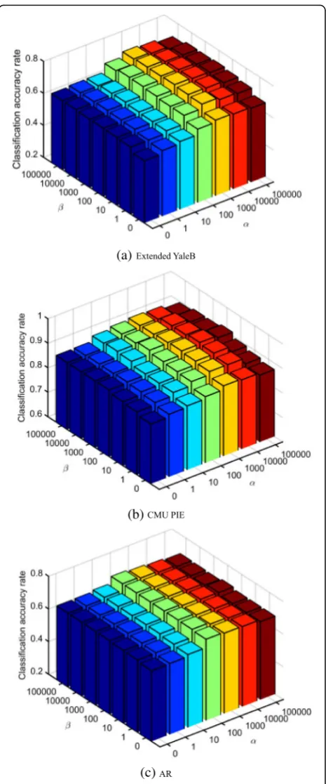
In the third experiment, the influence of two regularization parameters (i.e., αandβ) on the perform-ance of our DRMFFS is evaluated. We first set the same initialization for different parameters and then test the
impact of varying the values of parameters α and β on
the performance of the proposed approach. Figure 5
de-picts the classification results on three databases under different values ofαand β. As shown in Fig.5, the clas-sification results of the proposed approach change little
under different values of α and β on all the databases,
which indicates that our approach is insensitive to the
choice of parameters α and β. The average recognition
rates obtained by our DRMFFS are 0.7277 ± 0.0086 (290), 0.9233 ± 0.0105 (250), and 0.7040 ± 0.0115 (300) for the Extended YaleB, CMU PIE, and AR databases, re-spectively, which are higher than the results obtained by the newest approaches, i.e., NSSRD, JGSC, and JGSC, which are listed in Table 3. These results indicate that incorporating both the geometric structure information of the feature space and the correlation among features together are of great importance for feature selection, which can improve the classification performance.
Meanwhile, when the value ofβ is set to zero and α is
set to a non-zero value, the recognition rates obtained by DRMFFS are relatively higher than those obtained when settingαto zero. Specially, when the value ofαis set to zero, our approach is inferior to those obtained under other non-zero settings since the local structure information of the feature space of the data is totally neglected. Therefore, the preserving of the local struc-ture information of the feastruc-ture space of the data is im-portant for feature selection. In addition, a relatively largeα value or a relatively smallβvalue will cause the second term of the objective function in (7) to dominate
and overlook the other two terms. A relatively large β
value or a relatively small α value will cause the third
Table 3The average recognition rates and standard deviations of different algorithms on different databases. The best results are highlighted in italics
Methods Extended YaleB CMU PIE AR
Baseline 0.6193 ± 0.0081(1024) 0.8563 ± 0.0072(1024) 0.6206 ± 0.0162(1024)
LS 0.4850 ± 0.0142(500) 0.8196 ± 0.0180(500) 0.5851 ± 0.0155(500)
SPEC 0.6418 ± 0.0096(500) 0.8749 ± 0.0082(470) 0.6456 ± 0.0154(500)
MCFS 0.6589 ± 0.0178(200) 0.8791 ± 0.0084(490) 0.6521 ± 0.0158(500)
RUFS 0.6697 ± 0.0132(480) 0.8899 ± 0.0091(490) 0.6661 ± 0.0171(480)
MFFS 0.6722 ± 0.0093(330) 0.8862 ± 0.0088(270) 0.6741 ± 0.0147(470)
RSR 0.6883 ± 0.0106(500) 0.8937 ± 0.0085(440) 0.6671 ± 0.0147(440)
JGSC 0.6999 ± 0.0122(470) 0.8925 ± 0.0084(480) 0.6737 ± 0.0183(430)
SPNFSR 0.7190 ± 0.0077(180) 0.9184 ± 0.0103(430) 0.6895 ± 0.0117(270)
UDSFS 0.7195 ± 0.0095(490) 0.9167 ± 0.0159(400) 0.6931 ± 0.0144(240)
NSSRD 0.7202 ± 0.0119(440) 0.9185 ± 0.0096(410) 0.6979 ± 0.0152(430)
term of the objective function in (7) to dominate, and both the matrix factorization and the local structure in-formation of the feature space of the data will be neglected. All in all, the proposed approach can achieve
its best performance when the values ofαandβare
nei-ther too large nor too small. Moreover, we also can see that the varied performances are not caused by different
initializations, but the constraints that the initial settings are the same for varied parameters.
In the fourth experiment, we test the influence of initialization for our approach by randomly selecting a (a)
(b)
(c)
Fig. 4a–cThe recognition rates (%) of different feature selection algorithms on three different databases
(a)
(b)
(c)
set of training samples and testing samples from the AR, Extended YaleB, and CMU PIE databases. Meanwhile, we set the parameters of the algorithm as the optimal parameters. In this test experiment, we randomly gener-ate the matrices Aand P, then calculate the recognition rate of the algorithm. Here, the random generation process is repeated 30 times and the corresponding re-sult is shown in Fig.6. As seen from Fig.6, the recogni-tion rate of our approach is relatively stable at different initializations. Also, it demonstrates that our approach is insensitive to different initializations. The main reason is that our approach eventually converges under different initializations.
In the fifth experiment, we utilize the one-tailedttest to further verify whether DRMFFS performs significantly better than other approaches. In this test, the null hy-pothesis is that our DRMFFS makes no difference when compared to the existing unsupervised feature selection approaches in classification task and the alternative hy-pothesis is that our DRMFFS makes an improvement when compared to the other approaches. For example, if we want to compare the performance of DRMFFS with that of JGSC (DRMFFS vs. JGSC), the null and
alterna-tive hypotheses are defined as H0:MDRMFFS=MJGSC
andH1:MDRMFFS>MJGSC, respectively, where MDRMFFS and MJGSCare the average classification results obtained by DRMFFS and JGSC approaches on all of the three
Fig. 6The recognition rates (%) of DRMFFS vs. varying random initialization generation processes on three databases
Table 4Thepvalues of the pairwise one-tailedttests of DRMFFS and other approaches on classification accuracy
pvalues pvalues
DRMFFS vs. LS 9.1300e−05 DRMFFS vs. RSR 1.2334e−04
DRMFFS vs. SPEC 9.1300e−05 DRMFFS vs. JGSC 3.8458e−04
DRMFFS vs. MCFS 9.1336e−05 DRMFFS vs. SPNFSR 8.5006e−04
DRMFFS vs. RUFS 5.0123e−04 DRMFFS vs. UDSFS 0.0029
DRMFFS vs. MFFS 2.1976e−04 DRMFFS vs. NSSRD 0.0086
(a)
(b)
(c)
databases in Section 3.3. In our experiment, the signifi-cance level is set to 0.05. As seen from the test results depicted in Table4, thepvalues obtained by all the
pair-wise ttests are much less than 0.05, which means that
the null hypotheses are disapproved in all the pair-wiset
tests. Therefore, the proposed approach significantly outperforms other approaches.
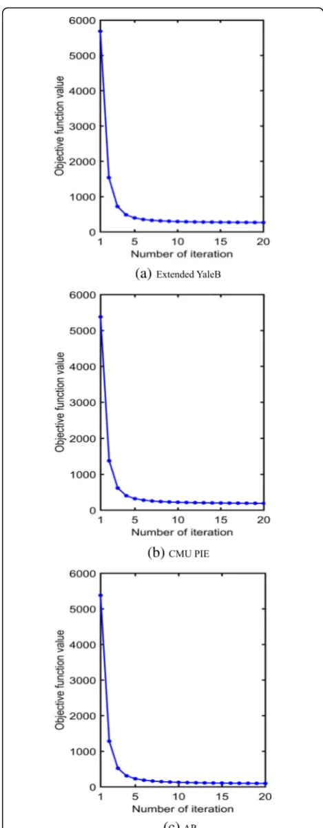
Finally, the convergence curves of the proposed ap-proach on three different databases are shown in Fig.7. As seen from these figures, the proposed approach con-verges very fast on all the databases, which demonstrates the efficiency and effectiveness of the proposed optimal approach.
3.4 Clustering results and analysis
In the clustering experiments, two widely used criteria, i.e., clustering accuracy (ACC) and normalized mutual information (NMI) are adopted to compare the cluster-ing performances of different unsupervised feature selec-tion approaches. The larger ACC or NMI is, the better
the performance of the algorithm, and vice versa. Given an input sample xi, let ci and gi be its clustering label and ground-truth label. The ACC can be formulated as
ACC¼ Xn
i¼1
γ gi;mapð Þci
n ð34Þ
whereγ(gi,ci) denotes an indicator function that equals 1 if ci=giand equals 0 ifci≠gi. Here,map(⋅) is the opti-mal mapping function that maps each clustering label to an equivalent true label by the Kuhn-Munkres algorithm [45].
NMI is defined as:
NMIðQ;RÞ ¼ ffiffiffiffiffiffiffiffiffiffiffiffiffiffiffiffiffiffiffiffiffiffiI Qð ;RÞ H Qð ÞH Rð Þ
p ð35Þ
where I(Q,R) represents the mutual information of Q
and R; the entropies of Q and R are, respectively,
Table 5Clustering results (ACC ± std) of different approaches on three different databases. The best results are highlighted in italics
Methods JAFFE ORL COIL20
BaseLine 0.7873 ± 0.0228(1024) 0.7526 ± 0.0439(1024) 0.5527 ± 0.0271(1024)
LS 0.8343 ± 0.0630(100) 0.7850 ± 0.0310(280) 0.5984 ± 0.0246(420)
SPEC 0.8521 ± 0.0708(470) 0.8030 ± 0.0756(170) 0.6128 ± 0.0476(340)
MCFS 0.8709 ± 0.0871(240) 0.8210 ± 0.0555(240) 0.6214 ± 0.0512(250)
RUFS 0.8864 ± 0.0781(470) 0.8300 ± 0.0542(140) 0.6408 ± 0.0484(360)
MFFS 0.8958 ± 0.0298(500) 0.8390 ± 0.0523(40) 0.6460 ± 0.0286(300)
RSR 0.8728 ± 0.0518(500) 0.8310 ± 0.0378(270) 0.6486 ± 0.0272(470)
JGSC 0.9004 ± 0.0557(280) 0.8460 ± 0.0332(240) 0.6537 ± 0.0402(200)
SPNFSR 0.9093 ± 0.0253(500) 0.8690 ± 0.0428(220) 0.6679 ± 0.0147(470)
UDSFS 0.9113 ± 0.0551(390) 0.8716 ± 0.0560(390) 0.6711 ± 0.0334(370)
NSSRD 0.9138 ± 0.0543(250) 0.8730 ± 0.0459(200) 0.6793 ± 0.0280(480)
DRMFFS 0.9226 ± 0.0254(130) 0.8833 ± 0.0320(430) 0.6853 ± 0.0162(380)
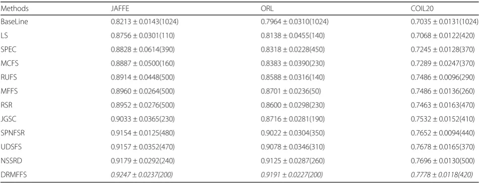
Table 6Clustering results (NMI ± std) of different approaches on three different databases. The best results are highlighted in italics
Methods JAFFE ORL COIL20
BaseLine 0.8213 ± 0.0143(1024) 0.7964 ± 0.0310(1024) 0.7035 ± 0.0131(1024)
LS 0.8756 ± 0.0301(110) 0.8138 ± 0.0455(140) 0.7068 ± 0.0122(420)
SPEC 0.8828 ± 0.0614(390) 0.8318 ± 0.0228(450) 0.7245 ± 0.0128(370)
MCFS 0.8887 ± 0.0500(160) 0.8383 ± 0.0390(230) 0.7289 ± 0.0247(370)
RUFS 0.8914 ± 0.0448(500) 0.8588 ± 0.0316(140) 0.7486 ± 0.0096(290)
MFFS 0.8960 ± 0.0264(500) 0.8701 ± 0.0236(50) 0.7486 ± 0.0136(260)
RSR 0.8952 ± 0.0276(500) 0.8600 ± 0.0298(230) 0.7463 ± 0.0163(470)
JGSC 0.9033 ± 0.0365(230) 0.8716 ± 0.0281(190) 0.7532 ± 0.0152(410)
SPNFSR 0.9154 ± 0.0125(480) 0.9022 ± 0.0304(350) 0.7652 ± 0.0094(440)
UDSFS 0.9157 ± 0.0352(470) 0.9078 ± 0.0346(310) 0.7678 ± 0.0165(370)
NSSRD 0.9179 ± 0.0292(240) 0.9125 ± 0.0287(260) 0.7696 ± 0.0130(500)
denoted as H(Q) and H(R). In this study, Q and R are the clustering label and the ground-truth, respectively.
According to the selected features, we utilize the
k-means algorithm to cluster all the samples, by different feature selection algorithms. Considering that the
per-formance of the k-means clustering approach relies on
the initialization, we repeat the process of clustering 50
times with different random initializations and the aver-age clustering results with standard deviations are given for this experiment. In this subsection, we use JAFFE, ORL, and COIL20 databases to evaluate the effectiveness of the proposed approach in terms of ACC and NMI.
First, we tune the number of the selected features from 10 to 500 with an interval of 10 to test the clustering
performance of different approaches. Tables 5 and 6
(a)
(b)
(c)
Fig. 8a–cThe ACC (%) of different feature selection algorithms on three different databases
(a)
(b)
(c)
report the best ACC and NMI from the optimal fixed
parameters obtained by different approaches. In Tables5
and 6, the number in parentheses is the number of the
selected features that corresponds to the best clustering
result. Since we use the same clustering experiment par-ameter setting with our previous work [21], the cluster-ing results of some compared approaches are the same
with [21]. Several interesting points can be observed
from Tables 5 and 6. First, all the feature selection
(a)
(b)
(c)
Fig. 10a–cThe ACC (%) of the proposed DRMFFS vs. parametersα andβon three different databases
(a)
(b)
(c)
approaches outperform than the baseline algorithm, in-dicating that feature selection plays an important role for clustering. Second, both LS and SPEC independently select features without considering the correlations among features. Therefore, their clustering performances are inferior to those of the sparsity regularized-based ap-proaches (i.e., MCFS, RUFS, RSR, SPNFSR, UDSFS, JGSC, NSSRD) and matrix factorization theory-based approaches (i.e., MFFS and our DRMFFS) on all the da-tabases. This indicates that they select the features in a batch manner which is more effective than individually. Although these approaches jointly select features and achieve better performance than LS and SPEC, they ei-ther ignore the geometric structure information of the feature space (i.e., MCFS, RUFS, SPNFSR, RSR, UDSFS, JGSC, MFFS), or the correlations among features (i.e., MCFS, RUFS, SPNFSR, RSR, JGSC, MFFS, NSSRD), which will greatly reduce the effectiveness of feature se-lection. Finally, it can be seen that our DRMFFS outper-forms the competing approaches. That is because the DRMFFS takes the geometric structure information of the feature space into the process of feature selection, making the selected feature subset more accurate. Fur-thermore, the DRMFFS has more advantages than the sparsity regularized-based approaches by replacing the
l1-norm or l2-norm with the inner product
regularization term that can be regarded as a
combin-ation of the l1-norm and l2-norm, such as considering
the correlations among features, achieving sparsity, and low redundancy simultaneously. All in all, our approach can achieve the best performance on all the databases, which demonstrates that the proposed approach is effective.
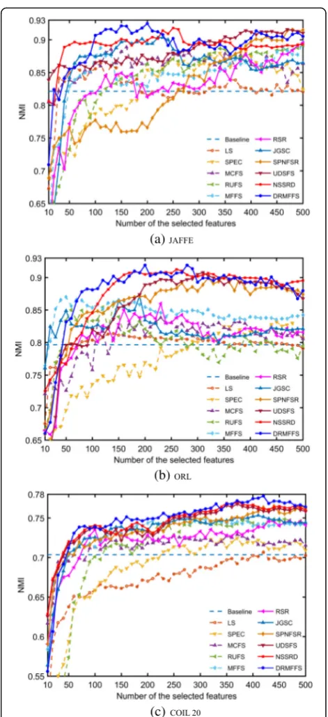
Second, the impact of various numbers of the selected features on the clustering performance (i.e., ACC and NMI) of different approaches is tested and the results
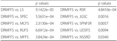
Table 7Thepvalues of the pairwise one-tailedttests on ACC
pvalues pvalues
DRMFFS vs. LS 9.1422e−05 DRMFFS vs. RSR 4.8410e−04
DRMFFS vs. SPEC 5.5631e−04 DRMFFS vs. JGSC 0.0016
DRMFFS vs. MCFS 2.3130e−04 DRMFFS vs. SPNFSR 0.0057
DRMFFS vs. RUFS 6.6912e−04 DRMFFS vs. UDSFS 0.0094
DRMFFS vs. MFFS 3.8424e−04 DRMFFS vs. NSSRD 0.0340
Table 8Thepvalues of the pairwise one-tailedttests on NMI
pvalues pvalues
DRMFFS vs. LS 9.1330e−05 DRMFFS vs. RSR 4.2793e−04
DRMFFS vs. SPEC 5.3208e−04 DRMFFS vs. JGSC 0.0014
DRMFFS vs. MCFS 1.0190e−04 DRMFFS vs. SPNFSR 0.0019
DRMFFS vs. RUFS 8.2529e−04 DRMFFS vs. UDSFS 0.0156
DRMFFS vs. MFFS 5.0210e−04 DRMFFS vs. NSSRD 0.0436
(a)
(b)
(c)
are shown in Figs.8and9. From the two figures, we can also observe that the clustering performances of our ap-proach are inferior to those of some other apap-proaches when the number of the selected features is small. The reason is the same as the classification experiments. However, with an increase of selected features, the pro-posed approach performs excellent and is finally
super-ior to all the compared approaches at higher
dimensions.
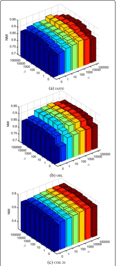
Next, similar to the classification experiment, we test the clustering performances of our approach under
vari-ous values of parametersαand β. Figures10and11
de-pict the clustering ACC and NMI, respectively, on the
three databases under different values of αand β. From
the results depicted in Figs. 10 and 11, we can easily
conclude the optimal values of parametersαandβfrom
the clustering experiments. When the parameters αand
β are set to 0, the correlations among features and the
local structure information of the feature space of the data are totally neglected. Under this circumstance, the average clustering ACC and NMI performances obtained by DRMFFS are inferior to those obtained under other parameter settings, which is consistent with the observa-tions in the classification experiments. Specially, when
the parameter α is set to 0, the performance of our
ap-proach is inferior to those obtained under other non-zero settings, indicating that the local structure in-formation of the feature space of the data is effective for improving the performance of feature selection. In addition, we can also see that our approach achieves its
best performance when the parameters α and β are set
to suitable values.
Furthermore, we also employ the one-tailed t test to
verify whether the clustering performance of DRMFFS is significantly better than the existing approaches. Here, we use the average of the clustering results (i.e., ACC and NMI) on all the databases for performance compari-son. We set the statistical significant level as 0.05 in this
experiment. The p values of the pairwise one-tailed t
tests on ACC and NMI are shown in Tables7 and8,
re-spectively. From these results, we can see that the p
values obtained by the pairwise one-tailedttests are less than 0.05, which indicates that our approach signifi-cantly outperforms other approaches.
At last, the convergence curves of our DRMFFS on
three different databases are shown in Fig. 12. From
these curves, it is easy to observe that the values of the objective function converge very fast, within approxi-mately 20 iterations, on all the three databases.
4 Conclusions
In this paper, we present a novel unsupervised feature selection approach called Double Regularized Matrix Factorization Feature Selection (DRMFFS) for image
classification and clustering. Since the feature manifold is important for dimensionality reduction, we utilize the graph regularization to preserve the manifold informa-tion of the feature space aiming to make the learning of feature selection matrix more accurate. Meanwhile, the absolute values of the inner product of the feature weight matrix vectors are employed as a regularization term to ensure high correlation and low redundancy among features simultaneously. Furthermore, we design the corresponding update algorithm to optimize our ap-proach and its convergence is also proved. In our experi-ments, the proposed approach is evaluated on six benchmark databases in terms of classification and clus-tering performances. The experimental results show that the proposed approach is effective.
Abbreviations
ACC:Clustering accuracy; DRMFFS: Double Regularized Matrix Factorization Feature Selection; GRNSR: Graph Regularized Nonnegative Self-Representation; JGSC: Joint Graph Sparse Coding; LS: Laplacian Score; MCFS: Multi-Cluster Feature Selection; MFFS: Matrix Factorization-Based Feature Selection; NDFS: Nonnegative Discriminative Feature Selection; NMF: Non-negative Matrix Factorization; NMI: Normalized mutual information; NSSRD: Non-Negative Spectral Learning with Sparse Regression-Based Dual-Graph Regularized Feature Selection; PCA: Principal Components Analysis; RSR: Regularized Self-Representation; RUFS: Robust Unsupervised Feature Selection; SPEC: Spectral Feature Selection; SPNFSR: Structure Preserving Nonnegative Feature Self-Representation; SVD: Singular Value Decomposition; UDFS: Unsupervised Discriminative Feature Selection; UDSFS: Unsupervised Deep Sparse Feature Selection;
UMMFSSC: Unsupervised Maximum Margin Feature Selection; VS: Variance Score
Acknowledgements
The authors would like to thank the editor, an associate editor, and referees for comments and suggestions which greatly improved this paper.
Availability of data materials
All of them are available. The links are listed as follows:
Extended YaleB database:http://vision.ucsd.edu/~iskwak/ExtYaleDatabase/ ExtYaleB.html
CMU PIE database:http://www.cs.cmu.edu/afs/cs/project/PIE/MultiPie/Multi-Pie/ Home.html
AR database:http://web.mit.edu/emeyers/www/face_databases.html#ar JAFFE database:http://www.kasrl.org/jaffe.html
ORL database:http://www.cad.zju.edu.cn/home/dengcai/Data/FaceData.html COIL20 database:http://www.cs.columbia.edu/CAVE/software/softlib/coil-20.php
Funding
Supported by the National Key R&D Program of China (no. 2017YFB1300900), National Natural Science Foundation of China (nos. U17132166, 61602221, 61603415 and 61701101), Natural Science Foundation of Jiangxi Province under grant (no. 20171BAB212009), Research Fund of Shenyang (no. 17-87-0-00), the Ph.D. Programs Foundation of Liaoning Province (201601019), and Fundamental Research Funds for the Central Universities (N172604004).
Authors’contributions
WZ, JW, and YY conceived and designed the experiments. WZ and YY performed the experiments. WZ, CW, and YY analyzed the data. CW and XY contributed reagents/materials/analysis tools. WZ and JW modified the manuscript. All authors read and approved the final manuscript.
Ethics approval and consent to participate Not applicable.
Competing interests
The authors declare that they have no competing interests.
Publisher’s Note
Springer Nature remains neutral with regard to jurisdictional claims in published maps and institutional affiliations.
Author details
1College of Information Science and Engineering, Northeastern University,
Shenyang 110819, China.2Faculty of Robot Science and Engineering,
Northeastern University, Shenyang 110819, China.3School of Information Science and Technology, Northeast Normal University Changchun, Changchun 130117, China.4Key Laboratory of Applied Statistics of MOE,
Northeast Normal University, Changchun 130117, China.5School of Software,
Jiangxi Normal University, Nanchang 330022, China.
Received: 27 December 2017 Accepted: 6 June 2018
References
1. JC Ang, A Mirzal, H Haron, HNA Hamed, Supervised, unsupervised, and semi-supervised feature selection: a review on gene selection. IEEE/ACM Transactions on Computational Biology & Bioinformatics
13(5), 971–989 (2016)
2. Y Yi, Y Shi, H Zhang, J Wang, J Kong, Label propagation based semi-supervised non-negative matrix factorization for feature extraction. Neurocomputing149(PB), 1021–1037 (2015)
3. D Cai, X He, J Han, TS Huang, Graph regularized nonnegative matrix factorization for data representation. IEEE Trans. Pattern Anal. Mach. Intell.
33(8), 1548–1560 (2011)
4. J Wang, W L, J Kong, et al., Maximum weight and minimum redundancy: a novel framework for feature subset selection. Pattern Recogn.46(6), 1616– 1627 (2013)
5. Y Li, CY Chen, WW Wasserman,Deep Feature Selection: Theory and Application to Identify Enhancers and Promoters, Proceedings of International Conference on Research in Computational Molecular Biology Springer(2015), pp. 205–217
6. H Peng, F Long, C Ding, Feature selection based on mutual information criteria of max-dependency, max-relevance, and min-redundancy. IEEE Trans. Pattern Anal. Machine Intell.5(8), 1226–1238 (2005)
7. M Hindawi, K Allab, K Benabdeslem,Constraint Selection-Based Semi-Supervised Feature Selection, Proceedings of IEEE 11th International Conference on Data Mining(IEEE, ICDM, Vancouver, BC, 2011), pp. 1080–1085 8. D Cai, C Zhang, X He,Unsupervised Feature Selection for Multi-cluster Data,
Proceedings of the 16th International Conference on Knowledge Discovery and Data Mining(ACM, SIGKDD, Washington, DC, 2010), pp. 333–342 9. Y Yang, HT Shen, Z Ma, Z Huang, X Zhou,l2,1-Norm Regularized
Discriminative Feature Selection for Unsupervised Learning, Proceedings of the International Joint Conference on Artificial Intelligence(AAAI, IJCIA, Barcelona, 2011), pp. 1589–1594
10. CM Bishop,Neural Networks for Pattern Recognition(Oxford University Press, Oxford, 1995)
11. X He, D Cai, P Niyogi,Laplacian Score for Feature Selection, Proceedings of International Conference on Neural Information Processing Systems(NIPS, Vancouver, British Columbia, 2005), pp. 507–514
12. Z Zhao, H Liu,Spectral Feature Selection for Supervised and Unsupervised Learning, Proceedings of the 24th International Conference on Machine Learning(ACM, Corvallis, OR, 2007), pp. 1151–1157
13. Y Cong, S Wang, B Fan, Y Yang, Y H, UDSFS: unsupervised deep sparse feature selection. Neurocomputing196(5), 150–158 (2016)
14. Z Li, Y Yang, J Liu, X Zhou, H Lu,Unsupervised Feature Selection Using Nonnegative Spectral Analysis, Proceedings of the Twenty-Sixth Conference on Artif. Intell(AAAI, Toronto, Ontario, 2012), pp. 1026–1032
15. S Yang, C Hou, F Nie, W Y, Unsupervised maximum margin feature selection via l2, 1-norm minimization. Neural Comput. & Applic.21(7), 1791–1799 (2012)
16. M Qian, C Zhai,Robust Unsupervised Feature Selection, Proceedings of the Twenty-Seventh AAAI Conference on Artificial Intelligence(AAAI, Bellevue, Washington, 2013), pp. 1621–1627
17. Y Yi, W Zhou, C Bi, G Luo, Y Cao, Y Shi, Inner product regularized nonnegative self representation for image classification and clustering. IEEE Access5, 14165–14176 (2017)
18. P Zhu, W Zuo, QH L Zhang, SCK Shiu, Unsupervised feature selection by regularized self-representation. Pattern Recogn.48(2), 438–446 (2015) 19. Y Yi, W Zhou, Y Cao, Q Liu, J Wang,Unsupervised Feature Selection with
Graph Regularized Nonnegative Self-Representation, Proceedings of the 11th Chinese Conference on Biometric Recognition, CCBR(Springer, Chengdu, 2016), pp. 591–599
20. W Zhou, W C, Y Yi, G Luo, Structure preserving non-negative feature self-representation for unsupervised feature selection. IEEE Access5(1), 8792– 8803 (2017)
21. X Zhu, X Li, CJ S Zhang, X Wu, Robust Joint Graph Sparse Coding for unsupervised Spectral Feature Selection. IEEE Transactions on Neural Networks & Learning Systems28(6), 1263–1275 (2017)
22. F Nie, W Zhu, X Li,Unsupervised Feature Selection with Structured Graph Optimization, Proceedings of Thirtieth AAAI Conference on Artificial Intelligence (AAAI, Phoenix, Arizona, 2016), pp. 1302–1308
23. R Shang, W Wang, R Stolkin, L Jiao, Non-negative spectral learning and sparse regression-based dual-graph regularized feature selection. IEEE Trans. Cybern.48(2), 1–14 (2018)
24. I Jolliffe Principal Component Analysis, Springer 7 (1986) 25. DD Lee, H Seung,Algorithms for Non-negative Matrix Factorization,
Proceedings of Advances in Neural Information Processing Systems(MIT, Denver, CO, 2000), pp. 556–562
26. S Lipovetsky, WM Conklin, Singular value decomposition in additive, multiplicative, and logistic forms. Pattern Recogn.38(7), 1099–1110 (2005) 27. S Wang, W Pedrycz, W Zhu, W Zhu, Subspace learning for unsupervised
feature selection via matrix factorization. Pattern Recogn.48(1), 10–19 (2015) 28. M Qi, T Wang, F Liu, B Zhang, J Wang, Y Yi, Unsupervised feature selection
by regularized matrix factorization. Neurocomputing23(17), 593–610 (2017) 29. N Zhou, Y Xu, H Cheng, J Fang, W Pedrycz, Global and local structure
preserving sparse subspace learning. Pattern Recogn.53(C), 87–101 (2016) 30. R Shang, W Wang, R Stolkin, L Jiao, Subspace learning-based graph
regularized feature selection. Knowl. Based Syst.112, 152–165 (2016) 31. K Lee, J Ho, D Kriegman, Acquiring linear subspaces for face recognition under
variable lighting. IEEE Trans. Pattern Anal. Mach. Intell.27(5), 684–698 (2005) 32. S Terence, B Simon, B Maan, The CMU pose, illumination, and expression (PIE)
database. IEEE Trans. Pattern Anal. Mach. Intell.25(12), 1615–1618 (2003) 33. AM Martinez, The AR Face Database. CVC Technical Report, 24 (1998) 34. M Lyons, S Akamatsu, M Kamachi, J Gyoba,Coding Facial Expressions with
Gabor Wavelets, Proceedings of IEEE International Conference on Automatic Face and Gesture Recognition(IEEE, Nara, 1998), pp. 200–205
35. FS Samaria, AC Harter,Parameterisation of a Stochastic Model for Human Face Identification, Proceedings of the Second IEEE Workshop on Applications of Computer Vision(IEEE, Sarasota, Florida, 1995), pp. 138–142
36. SA Nene, SK Nayar, H Murase, Columbia object image library (COIL-20). Technical Report, CUCS-005-96 (1996)
37. Q Han, ZG Sun, HW Hao, Selecting feature subset with sparsity and low redundancy for unsupervised learning. Knowl. Based Syst.86, 210–223 (2015) 38. F Shang, FW LC Jiao, Graph dual regularization non-negative matrix
factorization for co-clustering. Pattern Recogn.45(6), 2237–2250 (2012) 39. B J, P Li, C Chen, Z He, D Cai, Relational multi-manifold co-clustering. IEEE
Trans. Cybern.43(6), 1871–1881 (2013)
40. J Ye, Z Jin, Dual-graph regularized concept factorization for clustering. Neurocomputing138, 120–130 (2014)
41. J Wang, Y Yi, W Zhou, Y Shi, M Qi, M Zhang, Locality constrained joint dynamic sparse representation for local matching based face recognition. PLoS One9(11), e113198 (2014)
42. Y Yi, W Zhou, J Wang, Y Shi, J Kong, Face recognition using spatially smoothed discriminant structure-preserved projections. Journal of Electronic Imaging23(2), 1709–1717 (2014)
43. C Ding, T Li, MI Jordan, Convex and semi-nonnegative matrix factorizations. IEEE Trans. Pattern Anal. Mach. Intell.32(1), 45–55 (2010)
44. R Remmert, inSpringer Science & Business Media. Theory of complex functions (2012)