Songxiao Cao
*, Xuanyin Wang and Ke Xiang
Abstract
This paper presents a novel particle filter called Motion-Adaptive Particle Filter (MAPF) to track fast-moving objects that have complex dynamic movements. The objective was to achieve effectiveness and robustness against abrupt motions and affine transformations. To that end, MAPF first predicted both velocity and acceleration according to prior data of the tracked objects, and then used a novel approach called sub-particle drift (SPD) to improve the dynamic model when the target made a dramatic move from one frame to the next. Finally, the propagation distances of each direction in the dynamic model were determined based on the results of motion estimation and SPD. Experimental results showed that the proposed method was robust for tracking objects with complex dynamic movements and in terms of affine
transformation and occlusion. Compared to Continuously Adaptive Mean-Shift (CAM-Shift), standard particle filter (PF), Velocity-Adaptive Particle Filter (VAPF), and Memory-based Particle Filter (M-PF), the proposed tracker was superior for objects moving with large random velocities and accelerations.
Keywords: Motion-adaptive model, Object tracking, Particle filter, Sub-particle drift
1 Introduction
Visual object tracking is becoming more and more important in many application fields nowadays, such as surveillance, robots, and human-computer interfaces [1–3]. However, it is still a challenging task to achieve reliable tracking due to erratic motions, occlusions, crowded background scenes, and different illuminations.
Many algorithms and methods have been proposed to track moving objects in video sequence, among which the mean shift (MS) and particle filter (PF) are frequently used. As a powerful tool in dealing with the non-linear and non-Gaussian problems, PF has been extensively studied for visual object tracking [4–9].
1.1 Motion-adaptive problem of tracking
Most PF-based trackers use the linear Gaussian dynamic model as their target motion model. However, this sim-ple model cannot match the comsim-plexity of a fast-moving object with random velocity and acceleration.
This research aims to develop a robust tracker that could stably track a fast-moving rigid object with an unknown complexity dynamic model, which means that, even the target moves rapidly and changes abruptly in the moving direction, velocity, and accel-eration, the tracker will still keep up with the target closely. To that end, the main focus was put on propagating the particles in a better way so as to make them fit the non-linear, non-Markov, and time-variant dynamic, because an accurate propagating region is important not only for the accurate estima-tion of the target state, but also for the recovery from tracking loss caused by occlusions. This paper proposed a novel PF called Motion-Adaptive Particle Filter (MAPF), which could predict both velocity and acceleration based on the past data of the tracked object, and introduced a novel method called sub-particle drift (SPD) to improve the performance of the tracker during the target’ dramatic motion from one frame to the following. The SPD was done by weighting samples of a main particle set and four sub-particle sets (left, right, up, and down sides of * Correspondence:[email protected]
State Key Laboratory of Fluid Power and Mechatronic Systems, Zhejiang University, Hangzhou, China
the main particle set), as well as the drift to the dir-ection with a higher weight. A MAPF moving-object tracking was implemented in the adaptive color-based particle filter [6], which can also be used in many other particle filters where the velocity and acceler-ation of tracked objects should be considered.
1.2 Related works
In order to successfully track visual objects with complex dynamic movements, several extensions of the PF have been proposed including the random walk model and some other adaptive models. These PF-based trackers can be categorized as follows.
First, a training and learning process was employed for generating a dynamic model. Isard and Blake [10] used learned dynamics in the CONDENSATION algorithm to track moving objects. North and Blake [11] also got a dynamic model through learning to use the Expectation-Maximization CONDENSATION (EM-C) algorithm. Besides, Hess and Fern [12] proposed a discriminating training method for PFs. All of these methods may have good performance in tracking objects that have similar dynamic models with the trained video sequences. However, they are not very effective in tracking the arbitrarily moving objects which have not been previously learned, because the parameters used in the dynamic model are set to be constant values according to the trained video sequences. As a result, if the tracking object in a new test video sequence moves much faster or slower than the trained dynamic model, the tracking will end up with failure.
Second, a fixed constant-velocity model with fixed noise variance was used in a number of target trackers [13, 14] to propagate the particles between the frames. The result showed that a small velocity factor would lead to tracking loss when the target moved quickly, while, in case of a slow motion, it would cause drifting to back-ground which was similar to the target.
Third, some adaptive strategies have been proposed to deal with the complex dynamics. Zhou [15] used an adaptive-velocity model, where the adaptive mo-tion velocity was predicted using a first-order linear approximation based on the appearance difference between the incoming observation and the previous particle configuration, and the equation θt =θt‐1 +νt +Ut was used as the adaptive state transition model, where νt is the predicted shift in the motion vector and Ut is the adaptive noise parameter. Lui [16] de-termined the amount of observation noise based on the temporal difference of each state parameter and formulated the noise propagation distance in the dy-namic model as ∑u= max(a+b(ut−ut−1)), where a
ensures that a minimum amount of noise will be
added to an observation, and b weighs the temporal difference, which is set to be a constant value. Del Bimbo [17] proposed a PF-based tracker to exploit a first order dynamic model and continuously adapt the model noise so as to balance uncertainties between the static and dynamic components of the state vec-tor, which was formulated as θt =Aθt‐1 +νt‐1,where
νt‐1 is an additive, zero mean, and isotropic Gauss-ian uncertainty term. All the three papers used the velocity-adaptive model as the system dynamic model, called Velocity-Adaptive Particle Filter (VAPF). A Memory-based Particle Filter (M-PF) proposed by Mikami [18] introduced a paradigm called memory-based prior prediction which used the prior data of a target to predict prior distribution. The main idea of M-PF is to predict the prior distribution of the target state in future steps by weighing samples of the past sequence of target states, where the sample weight is determined based on the long-term dynamics of the targeted system. These approaches can effectively track targets that move relatively quickly, since they automatically change the propagation distance accord-ing to the estimated velocity. All of the algorithms can only adapt to small velocity changes of the target, but, when the target moves with a large acceleration, changing position, pose, and size dramatically from one frame to the following, they tend to end up with failure.
Fourth, spatial and temporal information or multi-scale strategies have been used in some other trackers. Yang [19] proposed a new search method for the estima-tion of consistent moestima-tion and disparity based on particle filtering, where the state dynamics involves the states of the neighboring blocks located in both spatial and tem-poral neighborhoods, which is similar to the method in this paper. However, Yang’s method focuses on estima-tion of consistent moestima-tion and is used in applicaestima-tions such as image reconstruction and video coding, making it less suitable for tracking targets with large velocity and acceleration and unknown complex dynamics, which is the target of the present research. Han [20] used an analytic approach to better approximate and propagate density functions with a mixture of Gaussians. This approach used unscented transformation to derive a mixture representation of the predicted probable distribution function and applied a multistage sampling strategy to approximate the likelihood function. However, the random walk model was still used as the process model, which can only deal with simple and slow motions of objects, but is not appropriate for com-plex dynamics.
Section 2 summarizes related methods used for visual object tracking; Section 3 deals with the MAPF; Section 4 introduces experimental results and makes comparisons with the Continuously Adaptive Mean-shift (CAM-Shift) [21], standard PF [6], VAPF [15, 16], and M-PF [18]; and Section 5 outlines the conclusions and suggestions for future research.
2 Color-based PF
This section briefly overviews the main concepts of related methods that are discussed in this paper, in-cluding the color distribution model used in all of the discussed methods, the basic formulae of the PF used for visual tracking, and the velocity-adaptive model.
2.1 Color distribution model
To achieve robustness against non-rigidity, rotation, and partial occlusion, the color distribution is a widely used target representation model. Because the intensity channel V is susceptible to illumin-ation variillumin-ations, a lot of models choose histograms of h×s bins in H-S two-dimension color space to represent the color distribution. To increase the re-liability of the color distribution when boundary pixels resembles the background of the occluded, smaller weights are assigned to the pixels that are further away from the region center by employing a weighting function:
k rð Þ ¼ 1−r
2 : r<1
0 : otherwise
ð1Þ
The color distribution py¼ pð Þyu
n o
u¼1…m at loca-tionyis calculated as:
pð Þyu ¼ChX
nh
i¼1
k y−xi a
δ½b xð Þ−i u ð2Þ
where f gxi i¼1;…nh is the normalized pixel location of the
target candidate, m= 16 × 8 is the bin used in the color distribution in this paper, nh is the number of pixels in
the region, b(xi) is the function which assigns the color
at location xi to the corresponding bin, a is the
parameter used to adapt the size of the region, and δis the Kronecher delta function. The normalization con-stant is calculated as:
Ch¼Pnh 1
i¼1k
y−xi a
ð3Þ
which ensures that p yð Þ ¼Pmu¼1puð Þ ¼y 1. Because the
pu(y) is the normalized distribution, its total sum
should be 1.
Fig. 2Circular template model
To measure the similarity between distributions p
= {pu}u= 1…m and q= {qu}u= 1…m, where m is the number of bins, the Bhattacharyya distance is adopted:
d¼pffiffiffiffiffiffiffiffiffiffiffiffiffiffiffiffiffiffi1−ρ½p;q ð4Þ
where
ρ½p;q ¼X
m
u¼1
ffiffiffiffiffiffiffiffiffiffi puqu p
ð5Þ
2.2 Particle filter
PF is a Monte Carlo approximation to the optimal Bayesian filter and provides robust tracking of moving objects in a cluttered environment, especially in the case
of non-linear and non-Gaussian problems where the interest lies in the detection and tracking of moving objects. It is a probabilistic framework for sequentially estimating the target’s state to recursively computer the posterior density p(st|z1 :t) of current object state st
-conditioned on all observations z1 :t= (z1,z2……zt) up to
timet.
To implement a standard PF, a state representation st
should be identified that, in object tracking, might in-clude object locations, scales, and rotations. Moreover, it is necessary to design three distributions: the process dy-namical distribution p(st|st−1), which describes how the object moves between frames; the proposal distribution
q(st|s1 : t−1,z1 :t), which is sampled each time the particle
distribution updates; and the observation likelihood distri-bution p(zt|st), which means how the object appears in the video frame.
This paper focuses on the dynamical distributionp(st|
st−1), which can usually be represented as a linear stochastic differential function:
st¼Ast−1þBωt−1 ð6Þ
whereAdefines the deterministic component of the dy-namic model;stis the state vector of timet;ωt−1∈(0, 1) is the system noise, which is usually a uniformly random variable or a multivariate Gaussian random variable; and
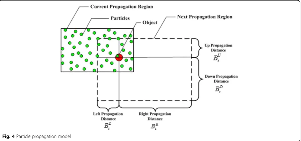
B is the propagation distance, indicating how far away the particles can propagate in the next frame and deter-mining the tracking performance when the object makes an arbitrary move.
Fig. 4Particle propagation model
As mentioned before, there are three different methods in dealing with the dynamic model: training and learning, a fixed constant-velocity model, and a vel-ocity adaptive model. In the training and learning method, the propagation distance B is determined through training and learning using some video se-quences, while, in a fixed constant-velocity model, B is set to be a constant value during the tracking process, and, as an adaptive method, the velocity adaptive model (VAPF) updates the propagation distance according to the temporal difference of previous frames by calculating the average velocity:
st ¼
1
j Xt
n¼t−j
∣sn−sn−1∣ ð7Þ
B0t∝s0t ð8Þ
wheres0t means the average state velocity in the previous
j frames of one certain dimension, and B0t is the corre-sponding propagation distance in that dimension. For
example, in thexdirection,Bx t∝xt ¼1j
P
n¼t−j
t
∣xn−xn−1∣.
The main advantage of the PFs mentioned above is its ro-bust performance under clutter background or occlusion. The main drawback is that it still cannot effectively track objects moving with rapid speeds and large accelerations.
3 The proposed method
This section describes the proposed MAPF used for vis-ual object tracking in complex dynamics, including the template model of the tracked objects (bounding rect-angular model and circular model), and the proposed motion-adaptive model.
Fig. 6Sub-particle model
3.1 Template model
As the proposed method is based on adaptive color-based PF, the tracking process is accomplished by choosing an appropriate bounding region as the area of interest out of some candidate regions and comparing the similarity of the color distribution between each other. In this paper, two different template modes, the rectangular model and circular model, were used according to the tracked object’s template.
3.1.1 Rectangular template model
In this model, a candidate bounding box can be de-scribed as:
s¼½x;y;w;h;θT ð9Þ where x,y represents the location of the rectangle, w,h
the width and height of the rectangle, andθthe rotation angle, as is described in Fig. 1. Thus, the track region
Fig. 8Particle weights distribution of the 7th frame of video“tennis”using different algorithms, PF(a), VAPF(b), M-PF(c) and Proposed(d)
can be represented by four vertices {P0,P1,P2,P3} of the rectangle, of which the corresponding coordinates are{(x0,y0), (x1,y1), (x2,y2), (x3,y3)}:
x0 x1 x2 x3 2 6 6 4 3 7 7 5¼ x x x x 2 6 6 4 3 7 7 5þ
Rsinðφ−θÞ
Rsinðπ−φ−θÞ
Rsinðπþφ−θÞ
Rsinð−φ−θÞ
2 6 6 6 4 3 7 7 7
5 ð10Þ
y0 y1 y2 y3 2 6 6 4 3 7 7 5¼ y y y y 2 6 6 4 3 7 7 5þ
Rcosðφ−θÞ
Rcosðπ−φ−θÞ
Rcosðπþφ−θÞ
Rcosð−φ−θÞ
2 6 6 6 4 3 7 7 7
5 ð11Þ
whereR¼1 2
ffiffiffiffiffiffiffiffiffiffiffiffiffiffiffiffi w2þh2
p
,φ= arctan(w/h), and−π2≤θ≤π2. The state variablescan be separated into two parts,sp
= [x,y]T and sa= [w,h,θ]T, where sp represents the ob-ject’s position-related parameters, whilesarepresents the affine transformations.
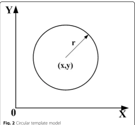
3.1.2 Circular template model
The circular model is relatively simple, in which a candi-date bounding circle can be described as:
s¼½x;y;rT ð12Þ
where x,y represents the location of the circle and rthe radius of the circle, as is described in Fig. 2. Then the tracking region can be represented by a circle centered in (x,y) with the radius r. As has been described above, the state variablesis separated into two parts, sp= [x,y]Tand
sa= [r]T, where sp represents the object’s position-related parameters, whilesarepresents the affine transformations.
3.2 Motion-adaptive model
In order to follow the tracked object moving with a com-plex dynamic, a motion adaptive model was proposed that combined velocity and acceleration estimation with a new approach called sub-particle drift.
3.2.1 Velocity and acceleration estimation
Settingvpt as the velocity vector at timetof the
position-related parameter andapt the acceleration vector, the fol-lowing formulae can be obtained:
vtp¼dsp=dt¼ðspt−spt−1Þ=T ð13Þ
apt ¼dvp=dt¼ðspt−2stp−1þspt−2Þ=T2 ð14Þ whereTis the sampling time andλT= 1/T:
vpt ¼λT spt−s p t−1
ð Þ ð15Þ
Fig. 10The tracking results using different parameters
apt ¼λ2T s p
t−2spt−1þs
p t−2
ð Þ ð16Þ
To reduce random noises, a weighted function was used for the velocityvpt and accelerationapt:
vpt ¼λT
XNs
n¼0
αnvpt−n ð17Þ
apt ¼λ2T
XNs
n¼0
βna p
t−n ð18Þ
whereαn and βnare the normalization factors for every
velocity and acceleration. And it was assumed that the older velocities and accelerations are assigned smaller weights:
XNs
n¼0
αn¼1
α0>α1>……>αn
8 < :
XNs
n¼0
βn¼1
β0>β1>……>βn
8 > < > :
ð19Þ
where Ns is the number of frames that needs to be smoothed.
Setting BpBase and BpMax as the base propagation and maximum propagation distance parameters of sp, respectively, the following formulae can be obtained:
BpMax¼BpBaseða
p t
2þ1Þ if ∣a
p t∣>Ta
BpMax¼BpBaseðv
p t
4þ1Þ else
8 > > > < > > > :
ð20Þ
Specifically, the base propagation distance BpBase, which consists of (Bx,By), is decided automatically ac-cording to the size of the tracked object. Take the rectangular template model as an example, as is seen in Fig. 3.
Ta is the acceleration threshold, which means that, when the acceleration at timetis larger than the thresh-old, the propagation radius is determined by apt , while
when the acceleration is smaller, it is determined by vpt.
Table 3Video sequences with different attributes
Attribute video OCC BC AT AM
Motians_chamber ✓
Bottle ✓
Book ✓ ✓
Basketball_1 ✓
Basketball_2 ✓ ✓
Basketball_3 ✓ ✓ ✓
Tennis ✓
v_juggle_11_06 ✓ ✓ ✓
v_juggle_15_02 ✓ ✓ ✓
Bolt ✓
Diving ✓
MountainBike ✓ ✓
RedTeam
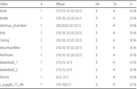
Table 2Parameter values used in the test
Video A BBase Ns Ta σ
Book 1 (15,15, 0.1,0.1,0.1) 3 4 0.16
Bottle 1 (10,10, 0.1,0.1,0.1) 3 4 0.16
Motinas_chamber 1 (20,20,0.1,0.1,0.1) 3 4 0.16
Bolt 1 (10,10, 0.1,0.1,0.1) 3 4 0.16
Diving 1 (10,10, 0.1,0.1,0.1) 3 4 0.16
MountainBike 1 (10,10, 0.1,0.1,0.1) 3 4 0.16
RedTeam 1 (10,10, 0.1,0.1,0.1) 3 4 0.16
Basketball_1 1 (15,15, 0.1) 3 4 0.16
Basketball_2 1 (15,15, 0.1) 3 4 0.16
Tennis 1 (5,5, 0.1) 3 4 0.16
v_juggle_11_06 1 (10,10,0.1) 3 4 0.16
Table 1Resulting of using different particle number
Sequences Number of Particles CAM-Shift PF VAPF Proposed
Book 100 138.83 34.69 11.40 7.05
150 34.99 18.68 9.99
200 62.47 17.30 5.02
250 35.15 77.15 5.41
300 34.06 20.79 5.13
Bottle 100 27.78 26.03 24.86 20.74
150 25.83 22.90 20.96
200 25.70 22.40 20.47
250 26.18 22.17 20.15
300 25.66 22.55 20.53
Basketball_1 100 78.58 71.09 53.59 14.90
150 88.28 85.50 16.51
200 88.76 44.12 9.93
250 87.36 36.48 8.34
300 65.65 65.83 8.35
Basketball_2 100 75.04 52.78 46.19 40.12
150 47.58 35.83 16.29
200 44.58 42.80 11.35
250 42.41 33.40 11.55
300 46.16 42.13 9.79
Tennis 100 116.31 136.04 80.47 2.31
150 15.24 13.96 2.27
200 80.78 79.07 2.04
250 80.47 79.24 2.18
The algorithm updates the propagation distance of each frame according to thevpt andapt,
Bpt ¼
Bxt 0 0 Byt
¼ BLt þBRt 0
0 BUt þBDt
" #
ð21Þ
while the affine transformation-related parameters Ba t
are all set to be one constant value. BL
t, BRt, BUt , and BDt
are the propagation distances of respectively the left, right, up, and down side based on the position of the ob-ject in the current frame, as is described in Fig.4.
And the distance of each side is determined based on the velocity or acceleration estimation. For example, in the horizontal movement, when the velocity or
acceleration is negative, that is, the object tends to move to the left side, the left propagation distance is set to be:
BL t ¼
BxMax¼Bxð ax
t
2þ1Þ if ∣a
x t∣>Ta
BxMax¼Bxðv x t
4þ1Þ else 8
> > > > < > > > > :
ð22Þ
while, in the opposite direction, the right propagation distanceBRt ¼BxBase.
Then, the dynamic model at timetcan be represented as:
st¼Ast−1þBtωt−1 ð23Þ
Fig. 12The tracking results for the video“bottle”using CAM-Shift (white), PF (blue), VAPF (green), M-PF (pink), and the proposed tracker (red). Particle numberN= 200
3.2.2 Sub-particle drift
In order to enhance the robustness of this research’s tracker for objects moving more dramatically, a sub-particle drift method is proposed. In this method, the center of the main particle set region drifts to the sub-particle set in which the
total particle weightP
i¼0
N
wiis the largest.
The sub-particle drift process is achieved by com-paring the particle weights and drifting to the max-imum in the next frame, as is described in the following formula:
wmax¼ max
XN
i¼0
wMi ;X
N
i¼0
wSPi 0……X
N
i¼0
wSPni
( )
ð24Þ
xtþ1
ytþ1
¼ xmaxt
ymax
t
ð25Þ
where wM
i and wSPni represent the particle weights of the
main and nth sub particle region, respectively, and
xmax
t , ymaxt are the x and y position with the largest
weight determined by Eq. (24). For example, when the second sub-particle set has the largest weight,
xmax
t ¼xSPt 1 and ymaxt ¼ySPt 1. Therefore, when the
maximum weight is in the main particle region, the propagation process is achieved according to Eq.(23); on the other hand, when the maximum region is one of the sub-particle sets, the dynamic model changes to the following:
st¼Asmaxt−1 þBtωt−1 ð26Þ
Fig. 14The tracking results for the video“basketball_1”using CAM-Shift (white), PF (blue), VAPF (green), M-PF (pink), and the proposed tracker (red). Particle numberN= 250
4 Results and discussion
To demonstrate the effectiveness and robustness of the proposed tracking scheme, 13 different color videos were used in the experiments (Additional files 1–13), which were obtained from different datasets. Four of them (Bolt, Diving, MountianBike, Redteam) belonged to the tracking benchmark dataset [22], three (basketall_1, basketall_2, basketall_3) were clips of the famous basketball dribbling teaching movie Bobbito’s Basics to
Boogie, two (v_juggle_11_06, v_juggle_15_02) from UCF
frame, and so was the corresponding template model. The proposed tracking method was also compared with the four existing trackers, CAM-Shift, PF, APF, and M-PF, to identify their correlations. All the algo-rithms were implemented in C++ using the OpenCV library and run on a 1.8 GHz Pentium Dual-Core CPU, with 2Gbyte DDR memory. The parameter T in Eq. (13) was T= 1/25 seconds because the video for-mat was PAL.
4.1 Parameters selection
There are some parameters that can affect the perform-ance of the proposed tracker. In order to achieve the best tracking performance, the process of selecting some parameters is discussed as follows.
1. Number of the sub-particle set
In this method, there are five different particle sets in the tracker, including one main particle set and four sub-particle sets (up, down, left, and right sub sets). All four sub-particle sets are generated by the main set and distributed as the main one is, except for the particle po-sitions. Take the rectangular template model as an ex-ample, as is described in Figs. 6 and 7.
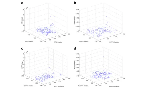
Figure 8 shows the particle weight distribution of PF (a), VAPF (b), M-PF (c), and proposed (d) of the 7th frame of the video “tennis.” It can be seen that the particles in PF are concentrated in a relatively small region and that VAPF propagates the particles in a larger scope, while the proposed tracker not only has five concentrated regions but also propagates in a lar-ger scope (Fig. 9).
2. Parameter A of the dynamic model
The equation of the circular model can be specified as follows:
xt yt rt 2 4
3
5¼
Axt 0 0
0 Ayt 0
0 0 Art 2
6 4
3 7 5 xytt−1−1
rt−1 2 4
3
5þ
Bx t 0 0
0 Byt 0
0 0 Brt 2
6 4
3 7 5 wwtt−1−1
wt−1 2 4
3 5
ð27Þ
The experiment results are shown in Fig. 10a, where the parameter A= 1 means Axt ¼Ayt ¼Art ¼1 .
It can be seen that the tracker performs best when the parameter Axt ¼Ayt ¼Art ¼1, because the
param-eter A in Eq. (23) shows the relationship between the Fig. 15The tracking results for the video“basketball_2”using CAM-Shift (white), PF (blue), VAPF (green), M-PF (pink), and the proposed tracker (red). Particle numberN= 250
object states of the current frame and the next one. Assuming that the position of one particle in the current frame is (100, 50), under the condition Axt
¼Ayt ¼1 , the particle is propagated to (100 + dom_x, 50 + random_y) in the next frame, where ran-dom_x and random_y are random values decided by the estimated velocity and acceleration. In contrast, under the condition Axt ¼Ayt ¼0:5 , the particle is propagated to (0.5 × 100 + random_x, 0.5 × 50 + rand-om_y), and it is obvious that the propagation process is not appropriate, so the tracking tends to fail.
3. Acceleration threshold
From the acceleration threshold curve of Fig. 10b, it can be found that, for the video sequence“Basketball_1,” the acceleration threshold between 3 and 7 pixels per frame2 tends to have a better tracking performance, while, for the
video sequence “Basketball_2,” all the tested thresholds are equally good. One explanation is that, in “Basket-ball_1,” the basketball moved much more dramatically. Most of the time, the ball moved from the top to the bot-tom of the image within 10 frames, having the video height of 240 pixels. According to the si¼12git2i , the image accelerationgiwas more than 2 pixels per frame2.
4. Particle number
For performance evaluation and comparison, all the four PF-based algorithms were tested using different numbers of particles, including 100, 150, 200, 250, and 300, and some of the tracking results are shown in Table 1. It can be found that the tracking performance improves when the particle number increases, and that it reaches the top when the particle number is larger than 200.
Fig. 17The tracking results for the video“v_juggle_11_06”using CAM-Shift (white), PF (blue), VAPF (green), M-PF (pink), and the proposed tracker (red). Particle numberN= 200
Other parameters used in the test are shown in Table 2. The following section first presents all the tracking results of the five algorithms in the same tested video with different color bounding boxes or circles and then performs detailed evaluations and comparisons to demonstrate the effectiveness of the algorithms.
4.2 Performance and results overview
To better evaluate and analyze the strength and weak-ness of the tracking approaches, the videos were catego-rized with four attributes based on the challenging factors including occlusion (OCC), background clutters (BC), affine transformation (AT), and abrupt motion (AM), as is seen in Table 3.
4.2.1 Occlusion
In the video sequences with the occlusion attribute, in general, all the four PF-based algorithms could recover from occlusion and loss when the object moved without abrupt motions, while differences showed up when the object moved abruptly.
In the video sequence “motinas_chamber,” the tracked object was a man in red. It can be observed
in Fig. 11 that, in the beginning, when the object ran slowly without occlusion, all tested algorithms tracked the object well, as can be seen in the 33rd frame, while, in the 93rd frame, when the object was oc-cluded by another person, the proposed tracker tracks the object better not only in position but also in size due to its accurate motion estimation. When the ob-ject disappeared from the field of view in the 717th frame and showed up again in the 746th, all the four PF-based algorithms recovered from loss, but, still, the proposed tracker performed a little better.
Tracking the basketball during dribbling was a very challenging task. Moreover, the partial or total occlusion made the tracking much more difficult when the player dribbled the ball behind the back or between the legs, as can be seen in the video“basketball_2.”In the 7th frame, when the basketball was blocked by his leg, the CAM-Shift and the PF lost its position, while the VAPF and the proposed tracker kept tracking it. And in the 33rd and 34th frames, when dribbled behind the back, the basketball was blocked by the back, but the proposed tracker had predicted this correctly and kept tracking the ball when it appeared again.
Fig. 19The tracking results for the video“Diving”using CAM-Shift (white), PF (blue), VAPF (green), M-PF (pink), and the proposed tracker (red). Particle numberN= 200
4.2.2 Background clutters
As all the four tested algorithms were based on color distribution, they could address the background clutter problem well in most cases. However, the weakness of color distribution showed up when there was another object in almost the same color as the true target, as can be seen in the video “basketball_3,” which will be dis-cussed in the section 4.2.3.
4.2.3 Affine transformation
In the video sequences with the affine transformation at-tribute, all four PF-based trackers could deal with the factor, while CAM-Shift’s bounding box was not tight due to its inability to follow the direction.
The video sequence “bottle” (Fig. 12) contained a fast moving bottle with affine transformation in a relatively simple background. Its dynamic model and background complexity was the simplest in all of the 13 tested vid-eos. At the beginning of the video sequence, the bottle moved with a relatively low speed and small
acceleration, as is shown in the 4th frame. All of the five tested algorithms performed almost equally well by tracking the object with the right position and rotation angle. When a relatively higher speed and bigger acceler-ation took place, as is shown in the 31st, 45th, and 46th frames, the VAPF and the proposed tracker showed their advantages compared with the CAM-Shift and the PF which could not follow the bottle well. Besides, the M-PF did not show any advantage because the video se-quence was too short and did not have much history data for constructing a better prior distribution.
4.2.4 Abrupt motion
In the video sequences with the abrupt motion attribute, including “book,” “basketball_1,” “basketball_2,” “ basket-ball_3,” “v_juggle_11_06,” “v_juggle_15_02,” and “Bolt,” the proposed algorithm performed the best because the velocity and acceleration was fully taken into account in the motion-adaptive model.
Fig. 21The tracking results for the video“RedTeam”using CAM-Shift (white), PF (blue), VAPF (green), M-PF (pink), and the proposed tracker (red). Particle numberN= 200
In the video sequence“book,”as can be seen in Fig. 13, the CAM-Shift lost track of the object in most of the 180 frames, except for the first few frames. Although the VAPF performed better than the PF, it still lost the object in a lot of frames, especially when a sudden direc-tion change occurred, as can be seen in the 91st frame. The M-PF did not follow the object well in the beginning because few history data were available, but performed much better after about 60 frames, as can be seen in the 91st, 124th, and 152nd frames. In compari-son, the proposed tracker managed to maintain smooth tracking despite sudden orientation changes and large acceleration (Figs. 14, 15, 16, and 17).
In the video“tennis,” the tennis ball first underwent a free fall and then bounced up several times. In the first few frames, all four algorithms tracked it well due to the low speed, while, in the later frames, they were affected by the acceleration of gravity, with the only exception of the proposed tracker which kept following the ball
because the acceleration had been fully taken into ac-count in the motion-adaptive model. The video “v_jug-gle_11_06”was even more challenging than the previous three because of the similarity in color between the soccer and the background, as well as the long-time total occlusion. From the 105th frame to the 117th, the soccer was totally occluded by the kid, during which all the four trackers kept searching around the position where they lost tracking, as can be seen in the 105th frame. When the ball appeared again, the four PF-based trackers recovered from loss and went on with the tracking. In contrast, the proposed tracker performed the best in fit-ting the right position and size, while the CAM-Shift got totally lost (Figs. 18, 19, 20, and 21).
4.3 Comparative performance analysis
The following section compares the performance of the MAPF with the four analyzed trackers using Euclidian distance, that is, the distance between the tracking pos-ition and the ground truth which is manually marked, to evaluate the tracking position accuracy.
4.3.1 Euclidian distance
Comparisons were made between the estimated tracking position, rotation angle, width, height, and the corre-sponding ground truth can be seen in Figs. 22, 23, 24, and 25. The results showed that the CAM-Shift performed the worst because it lost track of the object except in the first frames, and could not recover. The PF and the VAPF did maintain tracking, but could not make an accurate estimation of position, angle, or size, while the proposed tracker followed the position of the object in bothXandYdirections in most of the frames and fit-ted the object well both in rotation angle and width. However, the height result did not fit the ground truth very well because, in the video sequence of “book,” the height changed dramatically due to camera view and perspective. Besides, the tracking algorithm did not use Fig. 23Estimated object center position of“book”compared with ground truth with the particle numberN= 150
the same acceleration estimation strategy as the position related parameter in the target affine transformation.
Table 4 shows the result of the averaged Euclidian dis-tance d1 over all frames in all videos from both the pro-posed tracker and the four analyzed trackers, while Table 5 shows the d1 over all frames in each video from the two groups. For the four PF-based trackers, each data is the average value of the 100, 150, 200, 250, and 300 particles. The table showed that the PF-based tracker always performed better than the CAM-Shift ex-cept in some special cases, such as in “Basketball_1.” One explanation is that both the CAM-Shift and the PF lost the track of the object entirely, and, as a result, the positions of these two trackers tended to be random values, with one being possibly larger than the other. The performance of the proposed tracker was superior in all videos except the “bottle,” because the bottle moved relatively slowly and the background was simple, as can be seen in Fig. 12.
The rotation angle error between the tracking angle at timetand the ground truth angle can be described as:
e1t ¼ ∣θt−θGTt ∣ ð28Þ
whereθtis the rotation angle in one certain algorithm at
timetandθGTt is the ground truth in the same frame. The error between the estimated width at time t and the ground truth width can be described as:
e2t ¼ ∣Wt−WGTt ∣ ð29Þ
where Wtis the width of the tracked object in one
cer-tain algorithm at timetand WGTt is the ground truth in the same frame.
The error between the estimated height at time tand the ground truth height can be described as:
e3t ¼ ∣Ht−HGTt ∣ ð30Þ
where Ht is the height of the tracked object in one
cer-tain algorithm at timetand HGTt is the ground truth in the same frame.
Tables 6, 7, and 8 show the results of the averaged angle error e1, width error e2, and height error e3 over all frames in each video from the proposed tracker and four analyzed trackers. For the four PF-based trackers, each data is the average value of the results of 100, 150, 200, 250, and 300 particles. The videos used for the cir-cular template model were not analyzed in these three tables because there were no “angle,” “width,” and “height” in the model. These three tables show that the differences between the proposed tracker and the four analyzed trackers in the “book” were much more obvi-ous than those in the “bottle” and “motinas_chamber,” because the objects in the latter two videos moved Fig. 25Estimated width and height of“book”compared with ground truth with the particle numberN= 250
Table 5Resulting of averaged Euclidian distance
Video CAM-Shift PF VAPF M-PF Proposed
Book 138.83 40.27 29.06 10.88 6.52
Bottle 27.78 25.88 22.98 26.24 20.57
Motinas_chamber 67.97 18.87 16.82 24.48 13.07
Bolt 134.48 14.21 28.36 16.80 13.73
Diving 11.40 29.64 22.38 30.70 28.78
MountainBike 233.89 14.23 12.86 15.63 13.98
RedTeam 60.86 8.2 8.27 8.68 9.44
Basketball_1 78.58 80.23 57.10 17.20 16.58
Basketball_2 75.04 46.70 40.07 38.57 17.82
Tennis 116.31 78.48 52.67 64.24 2.17
v_juggle_11_06 55.78 21.20 21.11 24.70 19.64 Table 4Resulting of averaged position error of all test videos
Algorithms CAM-Shift PF VAPF M-PF Proposed
relatively slowly and did not have obvious affine trans-formation. Nevertheless, the trends in these tables still confirmed the robustness of the proposed tracker.
4.3.2 Time consumption
To evaluate the computational efficiency, the time used by every algorithm was recorded. For example, in the video “basketball_1,” as is seen in Fig. 26, when there were 150 particles, the PF and the VAPF needed about 60 ms per frame, the proposed tracker needed 50 ms, and the CAM-Shift only needed less than 1 ms. The sta-tistics showed that the proposed tracker was the most efficient among the four PF-trackers, saving about 16.7% time compared to the PF and the VAPF.
In the ordinary PF, every state vector {x,y,w,h,θ} of each particle in, for example, the rectangular model is generated by a random number generator, and every cycle involves a float number operation, which is really time-consuming. Compared with that, in the proposed method of the research, only the particles of the main region are generated by the random number generator, that is, 1/5 particles, while the other four regions are simply “duplicates” from the main region with the same distribution, which only need to change the position data {x,y}. The addition and subtraction operations are faster than the random number generating operation, making this method faster than the ordinary PF.
The time consumed by the M-PF tested in our experi-ments was much more than Mikami’s proposed in [18], because the latter’s algorithm could run 30.0 frames per second by using 2000 particles. The first reason for this large difference is that they employed the graphics pro-cessing unit (GPU) propro-cessing to accelerate the weight computation of particles, which was said to be 10 times faster than the CPU-only version used in the experi-ments of this research. Secondly, the Intel Core2Extreme 3.0GHz (Quad Core) CPU of the PC they used was much better. Therefore, the two hardware differences caused the huge difference in time consumption.
The proposed tracker, however, consumed much more time than the CAM-Shift, which was a common problem of PFs. Fortunately, the development of com-puter technology has provided many ways to solve the time consuming problem, such as to use parallel computing enabled by multi-core processors [25–28] and to use hash coding techniques to improve the ef-ficiency [29, 30].
4.3.3 Failure modes
In the tests, two failure modes were identified. In the first mode, there was another object which had almost the same template and motion parameters as the tracked one, as is seen in Fig. 27, while, in the second, the tracked object had similar color distribution as part of the background, as is seen in Fig. 28.
As all the four tested algorithms were based on color distribution, when there were nearby objects in the iden-tical color with the selected one or the background color distribution was similar to the object’s, the tracking process would probably end up with failure. In the first example, the man was dribbling two basketballs at the same time, and occlusion often took place when drib-bling behind the back or between legs, as can be seen in the 23rd and 83rd frames. In the 23rd frame, when the tracked basketball disappeared, the proposed tracker moved to another basketball immediately while the other Table 6Resulting of averaged angle error
Video CAM-Shift PF VAPF M-PF Proposed
Book 28.22 53.56 28.94 33.7 16.78
Bottle 8.53 16.35 10.23 17.33 11.02
Table 7Resulting of averaged width error
Video CAM-Shift PF VAPF M-PF Proposed
Book 36.65 5.09 13.41 4.27 3.12
Bottle 13.45 2.17 2.11 3.05 2.08
Motinas_chamber 196.21 6.86 6.54 11.28 6.50
Table 8Resulting of averaged height error
Video CAM-Shift PF VAPF M-PF Proposed
Book 19.19 7.39 5.34 4.41 4.37
Bottle 16.16 3.21 3.08 3.13 2.96
Motinas_chamber 59.73 17.03 17.05 29.23 15.44
four tended to stay in the original position and search, because the SPD mechanism of the proposed tracker detected a dramatic movement due to the similarity between the two basketballs. This was also the reason for the failure in the 170th, 196th, and 224th frames of the video “v_juggle_15_02,” which could be avoided by combing a much better appearance mode and ob-ject correspondence mechanism. However, finding a good template model for visual tracking remains a challenging task.
5 Conclusion
This paper has presented a MAPF for visual object tracking under complex dynamics. The ways of using the prior history position data to estimate the velocity and acceleration of moving objects were demonstrated,
and a new method called SPD was proposed to improve the robustness of tracking a fast-moving object. Through updating the propagation distance in the dynamic model in each frame, the robustness and effectiveness were significantly improved during the tracking process. The experimental results demonstrated that, compared with the CAM-Shift, PF, VAPF, and M-PF, the proposed algorithm was effective and robust in dealing with object tracking under conditions of complex dynamics, occlu-sion, and affine transformation. The tracking perform-ance was improved significantly not only in position accuracy and object similarity, but also in computational efficiency.
The proposed algorithm was inspired by the color-based PF and has turned out to be better, and it will be helpful in other PF algorithms that need to consider Fig. 27The tracking failure example of video“v_juggle_15_02”using CAM-Shift (white), PF (blue), VAPF (green), M-PF (pink), and the proposed tracker (red). Particle numberN= 250
objects moving with dramatic changes in velocity and acceleration.
6 Additional files
Additional file 1:Motinas_chamber. (MPG 18794 kb)
Additional file 2:Bottle. (MPG 554 kb)
Additional file 3:Book. (MPG 1830 kb)
Additional file 4:Basketball_1. (MPG 12150 kb)
Additional file 5:Basketball_2. (MPG 2604 kb)
Additional file 6:Tennies. (MPG 546 kb)
Additional file 7:V_juggle_11_06. (MPG 1882 kb)
Additional file 8:(Failure mode) Basketball_3. (MPG 1068 kb)
Additional file 9:(Failure mode) V_juggle_15_02. (MPG 3200 kb)
Additional file 10:Bolt. (MPG 3372 kb)
Additional file 11:Diving. (MPG 2208 kb)
Additional file 12:MountainBike. (MPG 2190 kb)
Additional file 13:RedTeam. (MPG 18430 kb)
Abbreviations
CAM-Shift:Continuously Adaptive Mean-Shift; MAPF: Motion-Adaptive Particle Filter; M-PF: Memory-based Particle Filter; PF: Standard particle filter; SPD: Sub-particle drift; VAPF: Velocity-Adaptive Particle Filter
Acknowledgements
The most heartfelt gratitude goes to Changwei Wu and Houqiang Zhao for their helpful discussion and feedback about the algorithm, as well as Fangge Lu for proofreading the English writing.
Funding
This research was supported in part by the Natural Science Foundation of China (NSFC) (Grant No: 51175459).
Availability of data and materials
The web links to the sources of the data (namely, images) used for our experiments and comparisons in this work have been provided in this article.
Authors’contributions
SC implemented the core algorithm, designed all the experiments, addressed the resulting data, and drafted the manuscript. XW participated in the design and construction of the motion-adaptive model and helped draft the manuscript. KX implemented the color distribution model and object template model and participated in designing the PF core algorithm. All authors have read and approved the final manuscript.
Ethics approval and consent to participate Not applicable.
Consent for publication Not applicable.
Competing interests
The authors hereby declare that they have no competing interests.
Publisher’s Note
Springer Nature remains neutral with regard to jurisdictional claims in published maps and institutional affiliations.
Received: 24 September 2016 Accepted: 2 November 2017
References
1. S Khan, M Shah,A Multiview Approach to Tracking People in Crowded Scenes Using a Planar Homography Constraint, Computer Vision—ECCV 2006 (Springer, Berlin,Heidelberg, 2006), pp. 133–146
2. A Yilmaz, Object tracking: a survey. ACM Comput. Surv.38(4), 81–93 (2006) 3. K. Cannons, A review of visual tracking. Dept. Comput. Sci. Eng. (2008) 4. NJ Gordon, DJ Salmond, AFM Smith, Novel approaches to
nonlinear/non-Gaussian Bayesian state estimation. IEE Proc. F-Radar Signal Process140(2), 107–113 (1993)
5. S Maskell, N Gordon, A tutorial on particle filters for on-line nonlinear/non-Gaussian Bayesian tracking. Target Track. Algorithms Appl2, 2/1–2/15 (2001) 6. K Nummiaro, E Koller-Meier, LV Gool, An adaptive color-based particle filter.
Image Vis. Comput21(1), 99–110 (2003)
7. Y Li, HZ Ai, T Yamashita, SH Lao, M Kawade, Tracking in low frame rate video: a cascade particle filter with discriminative observers of different life spans. IEEE Trans. Pattern Anal. Mach. Intell.30(10), 1728–1740 (2007) 8. J Kwon, KM Lee, FC Park, Visual tracking via geometric particle filtering on
the affine group with optimal importance functions. IEEE Conf. Comput. Vis. Pattern Recognit29, 991–998 (2009)
9. ZH Khan, IYH Gu, AG Backhouse, A robust particle filter-based method for tracking single visual object through complex scenes using dynamical object shape and appearance similarity. J. Signal Proc. Syst. Signal Image Video Technol65(1), 63–79 (2011)
10. M Isard, A Blake, Contour tracking by stochastic propagation of conditional density. Eur. Conf. Comput. Vis1064, 343–356 (1996)
11. B North, A Blake, M Isard, J Rittscher, Learning and classification of complex dynamics. IEEE Trans. Pattern Anal. Mach. Intell.22(9), 1016–1034 (2000) 12. R Hess, A Fern, Discriminatively trained particle filters for complex
multi-object tracking. IEEE Conf. Comput. Vis. Pattern Recognit, 240–247 (2009) 13. Y Wu, TS Huang, A co-inference approach to robust visual tracking. Eighth
IEEE Int. Conf. Comput. Vis2, 26–33 (2001)
14. MD Breitenstein, F Reichlin, B Leibe, E Koller-Meier, L Van Gool, Robust tracking-by-detection using a detector confidence particle filter. IEEE 12th Int. Conf. Comput. Vis, 1515–1522 (2009)
15. SHK Zhou, R Chellappa, B Moghaddam, Visual tracking and recognition using appearance-adaptive models in particle filters. IEEE Trans. Image Process.13(11), 1491–1506 (2004)
16. YM Lui, JR Beveridge, LD Whitley, Adaptive appearance model and condensation algorithm for robust face tracking. IEEE Trans. Syst. Man Cybern. Part a-Syst. Hum40(3), 437–448 (2010)
17. A Del Bimbo, F Dini, Particle filter-based visual tracking with a first order dynamic model and uncertainty adaptation. Comput. Vis. Image Underst. 115(6), 771–786 (2011)
18. D Mikami, K Otsuka, J Yamato, Memory-based particle filter for face pose tracking robust under complex dynamics. IEEE Conf. Comput. Vis. Pattern Recognit, 999–1006 (2009)
19. S Yang, Particle filtering based estimation of consistent motion and disparity with reduced search points. IEEE Trans. Circuits Syst. Video Technol 22(1), 91–104 (2012)
20. B Han, Y Zhu, D Comaniciu, LS Davis, Visual tracking by continuous density propagation in sequential Bayesian filtering framework. IEEE Trans. Pattern Anal. Mach. Intell.31(5), 919–930 (2009)
21. G. R. Bradski, Computer Vision Face Tracking For Use in a Perceptual User Interface. Intel Technology Journal, 2nd Quarter, 214–219 (1998) 22. Y Wu, J Lim, M-H Yang, Online object tracking: a benchmark. Proc. IEEE
Conf. Comput. Vis. Pattern Recognit, 2411–2418 (2013)
23. UCF YouTube Action Dataset. http://vision.eecs.ucf.edu/projects/liujg/ YouTube_Action_dataset.html. A ccessed 11 Apr 2015.
24. SPEVI dataset. http://www.eecs.qmul.ac.uk/~andrea/spevi.html. Accessed 11 Apr 2015.
25. C. Yan, Y Zhang, J Xu, et al. A highly parallel framework for HEVC coding unit partitioning tree decision on many-core processors[J]. IEEE Signal Process. Lett, 21(5),573-576 (2014).
26. C Yan, Y Zhang, J Xu, et al., Efficient parallel framework for HEVC motion estimation on many-core processors[J]. IEEE Trans. Circuits Syst. Video Technol24(12), 2077–2089 (2014)