Solving Nonlinear Evolution Equations by (G'/G)-Expansion Method

(1)

http://www.sciencepublishinggroup.com/j/optics doi: 10.11648/j.optics.20180701.17

ISSN: 2328-7780 (Print); ISSN: 2328-7810 (Online)

Methodology Article

Solving Nonlinear Evolution Equations by

(G'/G)

-Expansion

Method

Attia Rani

1

, Munazza Saeed

1

, Muhammad Ashraf

1

, Rakshanda Zaman

1

,

Qazi Mahmood-Ul-Hassan

1, *

, Kamran Ayub

2

, Muhammad Yaqub Khan

2

, Madiha Afzal

3

1

Department of Mathematics, University of Wah, Wah Cantt., Pakistan

2

Department of Mathematics, Riphah International University, Islamabad, Pakistan

3

Department of Mathematics, Allama Iqbal Open University, Islamabad, Pakistan

Email address:

*_{Corresponding author}

To cite this article:

Attia Rani, Munazza Saeed, Muhammad Ashraf, Rakshanda Zaman, Qazi Mahmood-Ul-Hassan, Kamran Ayub, Muhammad Yaqub Khan, Madiha Afzal. Solving Nonlinear Evolution Equations by (G'/G)-Expansion Method. Optics. Vol. 7, No. 1, 2018, pp. 43-53.

doi: 10.11648/j.optics.20180701.17

Received: June 24, 2018; Accepted: July 13, 2018; Published: August 8, 2018

Abstract:

Nonlinear mathematical models and their solutions attain much attention in soliton theory. In this paper, main focus is to find travelling wave solutions of foam drainage equation and NLEE of fourth order. (G'/G)-expansion method is applied on these nonlinear differential equations. Wave transformation is used to convert nonlinear partial differential equation into an ordinary differential equation. It is observed that (G'/G)-expansion method is advanced and easy tool for finding solution of NLEEs in engineering, optics and mathematical physics. The proposed method is highly effective and reliable.

Keywords:

(G'/G)-Expansion Method, Nonlinear Evolution Equations, Travelling Wave Solutions, Maple 18

1. Introduction

In the last few years, we have observed an extraordinary progress in soliton theory. Solitons have been studied by various mathematician, physicists and engineers for their applications in physical phenomena’s. Firstly soliton waves are observed by an engineer John Scott Russell. Wide ranges of phenomena in mathematics and physics are modeled by differential equations. In nonlinear science it is of great importance and interest to explain physical models and attain analytical solutions. In the recent past large series of chemical, biological and physical singularities are feint by nonlinear partial differential equations. At present the prominent and valuable progress are made in the field of physical sciences. The great achievement is the development of various techniques to hunt for solitary wave solutions of differential equations. In nonlinear physical sciences, an essential contribution is of exact solutions because of this we can study physical behaviors and discus more features of the problem

which give direction to more applications.

A reliable technique presented by Wang et al which is known as (G'/G)-expansion method for the nonlinear evolution equations (NLEEs) and provides the exact traveling wave solutions. In this technique, a linear ordinary differential

equation of second order is used,

(2)

rational hyperbolic and rational functions. The proposed method is powerful tool and very user-friendly for solving NLEEs. On exact solution some novel results and computational methods involved to travelling-wave transformation, see the references, [22-30].

2. Analysis of

′

/

-Expansion Method

The general form of nonlinear partial differential equation is

̅, ̅ , ̅ , ̅ , ̅ , ̅ , ̅ , ̅ , ̅ , ̅ , ̅ , ̅ , ̅ , ̅ , ̅ , … = 0. (1)

Here is a polynomial in , . The steps of (G´/G)-expansion method are as follows:

Step 1: Seek travelling wave variable of Eq. (1) by letting

̅ , = ̅ ̅ , ̅ = ! "# $% & .

and Eq. (1) transform into the ODE.

' ̅, ̅′, ̅′′, ̅′′′, … = 0.

(2)

Here primes are representing the derivative of ̅ with respect to ̅ and & denotes constant.

Step 2: Constant (s) of integration can be obtained by integrating Eq. (2) term wise one or more times, if possible. For minimalism, the integration constant (s) can be set equal

to zero.

Step 3: According to the given proposed algorithm, suppose that the wave solution can be written as follows

̅ = () ∑ (+,

-.

-/ + 0

+12 . (3)

Where is the solution of 1st order nonlinear equation in the following form:

= 0. (4) Where and are unknown constants. By using the general solution of Eq. (3), we get

-.₃

- 3 =

456₇₈₉

: ;

<=>?+@A=₆B567893CD<6<E>@A=₆B567893C

<=<E>@,=₆456789/D<6>?+@A=₆B567893CF −

5

:, :− 4 > 0. (5)

=4− :₂ 4 ;−K2LMN ,124− : 4 ̅/ K:KPL ,124− : 4 ̅/ K2KPL ,124− : 4 ̅/ K:LMN ,124− : 4 ̅/F − 2,

:_{− 4 < 0.}

=_K 2K2

2 K: ̅− 2,

:_{− 4 = 0.}

Where K₂, K_: are unknown constants and we have

A _̅ ̅ C = − RA C: A C S.

A ̅

̅ C = R2 A C

T

3 A C: : _{2 A C} _VS.

⋮

Where the primes represents the derivatives w.r.t ̅. To find out ̅ explicitly, we follow these four steps.

Step 4: Substituting Eq. (3) and (4) into Eq. (2) after that, collect all terms with the same order of ′/ _{together, the}

left-hand side of Eq. (1) is converted into a polynomial in

′/ _{. Then by setting each coefficient equal to zero in this}

polynomial yields a set of algebraic equations for !, ", $, &, W and (₊, N = 0,1, . . . , X.

Step 5: Solve this system of algebraic equations obtained for !, ", $, &, W and (₊, N =0,1, . . . , X by using MAPLE 18.

Step 6: Use the results obtained from above steps to get a series of fundamental solutions ̅ ̅ of Eq. (2) that is

depending on ,

-′

-/. Since the solutions of Eq. (3) will be well known for us, and then we can get the exact solutions of Eq.

(4).

3. Numerical Applications

We solve the following two problems to illustrate the implementation of the ′/ _{expansion method.}

3.1. Foam Drainage Equation

Consider the Foam drainage equation [8]

YZ Y

Y

Y [ :−

4Z :

YZ

Y \ = 0. (6)

(3)

intersection of three films, mostly indicated as Plateau border (liquid filled channels). We focus on quantitative description of the coupling of drainage. Foam drainage is the flow of liquid from Plateau borders and the point where four channels meet between the bubbles, derived from capillarity and gravity. In foam stability foam drainage plays an important role. In fact, structure of the foam becomes fragile, when foam dries. [21]

Using the transformation as = ] ̅ , ̅ = ^

& , where & and ^ are unknown constants, the given Eq. (6) is being transferred to

^&Y__Y3 ^_Y3Y ,]:₋`

:4]

Y_

Y3/ = 0. (7)

Integrating Eq. (7) once with respect to and setting integration constant equal to zero, we have

^&] ^ ,]:₋`

:4]

Y_

Y3/ = 0. (8)

By substituting ] ̅ = : ̅ , we have

^& : _{^ ,} 8₋^

2 . 2 / = 0.

Or equivalently

& :_{− ^ = 0.}

(9)

By using the homogenous principle we balance the and :, we get

X 1 = 2X, X = 1.

We assume equation Eq. (9) has the solution

= () (2,a

.

a/ , (2≠ 0. (10)

Here (₎ and (₂ are unknown constants to be find out later.

= ̅ satisfy the second order linear ordinary differential equation of the form

c _̅ _{VG ̅} _{e ̅ = 0.}₍₁₁₎

V and e are constants, from Eq. (11), we have

= f g g g g g h g g g g g i

4V:_{− 4e}

2 j k

l!2LMNℎ A4V :_{− 4e ̅}

2 C !:KPLℎ A4V

:_{− 4e ̅}

2 C

!2KPLℎ A4V :_{− 4e ̅}

2 C !:LMNℎ A4V

:_{− 4e ̅}

2 C_n

o p₋V

2 , V:− 4e > 0.

44e − V:

2 j k

l−!2LMNℎ A44e − V :_̅

2 C !:KPLℎ A44e − V

:_̅

2 C

!2KPLℎ A44e − V :_̅

2 C !:LMNℎ A44e − V

:_̅

2 C_n

o p₋V

2 , V:− 4e < 0.

2!2

!2 !: ̅−

V

2 , V: − 4e = 0.

Putting Eq. (10) into Eq. (9) and by collecting all terms with the same order of ,-_-./, we get a set of algebraic equations for

&, () and (2 as follows

AG_{G C}

)

: ω (): (2Ve = 0,

AG_{G C}2: 2()(2 (2V:= 0,

AG_{G C}:: (2: (2V = 0.

Constants &, (₎ and (₂ can be determined by using MAPLE 18, we have one solution set.

()= −2_:V:, (2= −V, & = −2₈V8 V:e. (12)

By using values of the above constants in Eq. (10), we get

= −V ,a_a./ −2_:V:_{, & = −}2

8V8 V:e. (13)

Case I: When V:− 4e > 0.

2= −s4s

6_78t

:

j k lu=>?+@;

Bv6wxyz{

6 FDu6<E>@; Bv6wxyz{

6 F

u=<E>@;Bv6wxyz{₆ FDu6>?+@;Bv6wxyz{₆ F

n o p_.

(14)

Here k₂ and k_:are arbitrary constants.

If !₂= 0, then solution (14) can be simplified as

:= −s4s

6_78t

: KP ℎ [

4s6_78t3

: \. (15)

If !_:= 0, then solution (14) can be simplified as

T= −s4s

6_78t

: (Nℎ [

4s6_78t3

: \. (16)

(4)

8= −s48t7s_: 6

j k

l7u=>?+@;Bxywv6z{₆ FDu6<E>@;Bxywv6z{₆ F

u=<E>@;Bxywv6z{₆ FDu6>?+@;Bxywv6z{₆ F

n o p

. (17)

If !₂ 0, then solution (17) can be simplified as

} Gs48t7s_: 6KP m [48t7s_: 63\. (18)

If !_: 0, then solution (17) can be simplified as

~ s48t7s

6

: (Nm [

48t7s6₃

: \. (19)

Case III: When V:G 4e 0.

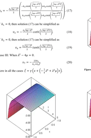
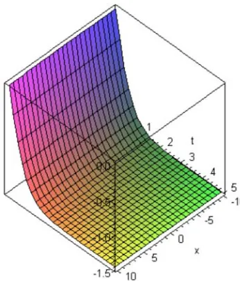
• G_u₌:su_Du=₆₃. (20)

Here in all the cases ̅ ^ , ,G2₈V8 V:e/ /.

Figure 1. Soliton solution of ₂ , for !₂ 1, !_: 1.5, ^ 1, V

3, e 1.

Figure 2. Soliton solution of ₂ , for !₂ 1, !_: 2.5, ^ 1.5, V

4, e 2.

Figure 3. Soliton solution of _: , for ^ 1, V 3, e 1.

Figure 4. Soliton solution of _: , for ^ 2, V 4, e 2.

(5)

Figure 6. Soliton solution of _T , for ^ 2.5, V 3, e 2.

Figure 7. Soliton solution of ₈ , for !₂ 1, !_: 1.5, ^ 2.5, V

3, e 3.

Figure 8. Soliton solution of ₈ , for !₂ 1.5, !_: 2, ^ 3, V

2, e 2.

Figure 9. Soliton solution of _} , for ^ 3, V 2, e 2.

Figure 10. Soliton solution of _} , for ^ 3.5, V 3, e 3.

(6)

3.2. Nonlinear Fourth Order Evolution Equation

Let us consider the NLEE of fourth order [13]

G ( • 0. (21) Where ( and • are constants. Fourth order NLEE is one of good starting point for study of non-linear water waves that was first point out by Dysthe in 1979. He obtained for gravity waves propagating at the interface of two superposed fluids of infinite depth over water in the presence of air flowing and a basic current sheer.

By using the transformation as ̅ = − & , we reduce the given Eq. (21) into an ODE

& c_{− (} c :_{− •} ?‚ _{= 0.}₍₂₂₎ By putting = c, we have

& − ( :_{− •} c_{= 0.}₍₂₃₎

Balancing the c and : by using the homogenous principle, we get

X 2 = 2X, X = 2.

Now, we suppose Eq. (23) has the solution

= () (2,a

.

a/ (:,

a. a/

:

, (:≠ 0. (24)

Here (₎, (₂ and (_: are constants to be find out later.

= ̅ satisfy the second order linear ordinary differential equation in the following form

c _̅ _{VG ̅} _{e ̅ = 0.}₍₂₅₎

V and e are constants, from Eq. (25), we get

G G =

f g g g g g h g g g g g i

4V:_{− 4e}

2 j k

l!2LMNℎ A4V :_{− 4e ̅}

2 C !:KPLℎ A4V

:_{− 4e ̅}

2 C

!2KPLℎ A4V :_{− 4e ̅}

2 C !:LMNℎ A4V

:_{− 4e ̅}

2 C_n

o p

−V_{2 , V}:_{− 4e > 0.}

44e − V:

2 j k

l−!2LMNℎ A44e − V :_̅

2 C !:KPLℎ A44e − V

:_̅

2 C

!2KPLℎ A44e − V :_̅

2 C !:LMNℎ A44e − V

:_̅

2 C_n

o p

−V_{2 , V}:_{− 4e < 0.}

2!2

!2 !: ̅−

V

2 , V: − 4e = 0.

By putting the Eq. (24) into eq. (23) and collecting all terms with the same order of ,-_-./ we yields a set of algebraic equations for &, (₎, (₂and (_: as follows

AG_{G C}): ω()− (():− •(2Ve − 2•(:e:= 0,

AG_{G C}2: ω(2− 2(()(2− •(2V:− 2•(2e − 6•(:Ve = 0,

AG_{G C}

:

: ω(:− 2(()(:− ((2:− 3•(2V − 4•(:V:− 8•(:e = 0,

AG_{G C}T: − 2((2(:− 2•(2− 10•(:V = 0,

AG_{G C}8: − ((::− 6•(:= 0.

Constants &, (₎, (₂ and (_: can be determined by using MAPLE 18, we have following two solution sets 1st Solution Set:

(:= −~…_†, (2= −~…s_† , ()= −~…t_† , & = −4•e •V:. (26)

(7)

G6•_{( A}G_{G C}:G6•V_{( A}G_{G C G}6•e₍ .

Case I: When V:− 4e > 0.

2= −3• ,s

6_78t

:† /

j k lu=>?+@;

Bv6wxyz{

6 F

n o p

:

−~…t_† . (27)

2= −3• ,s

6_78t

:† / ∬

j k lu=>?+@;

Bv6wxyz{

6 F

n o p

:

d ̅d ̅

3

) −T…t3

6

† . (28)

Where k₂ and k_:are arbitrary constants.

If !₂= 0, then solution (27) and (28) can be expressed as

:= −3• ,s

6_78t

:† / KP ℎ:[ 4s6_78t3

: \ −

~…t

† . (29)

:= −3• ,s

6_78t

:† / ∬ KP ℎ:[ 4s6_78t3

: \ ‰ ̅d ̅ − 3

) T…t3

6

† . (30)

If !_:= 0, then solution (27) and (28) can be expressed as

T= −3• ,s

6_78t

:† / (Nℎ:[ 4s6_78t3

: \ −

~…t

† . (31)

T= −3• ,s

6_78t

:† / ∬ (Nℎ:[ 4s6_78t3

: \ ‰ ̅d ̅ − 3

) T…t3

6

† . (32)

Case II: When V:− 4e < 0.

8= −3• ,8t7s

6

:† /

j k

n o p

:

−~…t_†6. (33)

8= −3• ,8t7s

6

:† / ∬

j k

lu=>?+@;Bxywv6z{₆ FDu6<E>@;Bxywv6z{₆ F

n o p

:

d ̅d { −T…t3_† 6.

3

) (34)

If !₂= 0, then solution (33) and (34) can be simplified as

}= −3• ,8t7s

6

:† / KP ℎ:[ 48t7s6₃

: \ −

~…t

† . (35)

}= −3• ,8t7s

6

:† / ∬ KP ℎ:[ 48t7s6₃

: \

3

) d ̅d ̅ −T…t3

6

† . (36)

If !_:= 0, then solution (33) and (34) can be simplified as

~= −3• ,8t7s

6

:† / (Nℎ:[ 48t7s6₃

: \ −

~…t

† . (37)

}= −3• ,8t7s

6

:† / ∬ (Nℎ:[ 48t7s6₃

: \

3

) d ̅d ̅ −T…t3

6

† . (38)

Case III: When V:− 4e = 0.

•= −24• u=

6

† Š=DŠ636−

~…t

† . (39)

•= −24• ∬ u=

6

† Š=DŠ636

3

) d ̅d ̅ −T…t3

6

† . (40)

(8)

2nd Solution Set:

() G… s

6_D:t

† , (2= −

~…s † ,

(:=7~…_† , & = −•V: 4•e.

‹ (41)

By substituting values of above constants in Eq. (24), we have

=−6•_{( A}G_{G C}:−6•V_{( A}G_{G C −}• V:₍ 2e .

Case I: When V:− 4e > 0,

Œ= −3• ,s

6_78t

:† /

j k lu=>?+@;

Bv6wxyz{

6 F

n o p

:

−… s6_†D:t. (42)

Œ= −3• ,s

6_78t

:† / ∬

j k lu=>?+@;

Bv6wxyz{

6 F

n o p

:

d ̅‰ ̅

3

) −

… s6_{D:t 3}6

:† . (43)

Where k₂ and k_:are arbitrary constants.

•= −3• ,s

6_78t

:† / KP ℎ:[ 4s6_78t3

: \ −

… s6D:t

† . (44)

•= −3• ,s

6_78t

:† / ∬ KP ℎ:[ 4s6_78t3

: \

3

) d ̅‰ ̅ −

… s6_{D:t 3}6

:† . (45)

If !_:= 0, then solution (42) and (43) can be simplified as

2)= −3• ,s

6_78t

:† / (Nℎ:[ 4s6_78t3

: \ −

… s6D:t

† . (46)

2)= −3• ,s

6_78t

:† / ∬ (Nℎ:[ 4s6_78t3

: \

3

) d ̅‰ ̅ −

… s6_{D:t 3}6

:† . (47)

Case II: When V:− 4e < 0,

22= −3• ,8t7s

6

:† /

j k

n o p

:

−… s6_†D:t. (48)

22= −3• ,8t7s

6

:† / ∬

j k lu=>?+@;

Bxywv6z{

6 FDu6<E>@; Bxywv6z{

6 F

n o p

:

d ̅‰ ̅ −… s6D:t 3_:† 6.

3

) (49)

2:= −3• ,8t7s

6

:† / KP ℎ:[ 48t7s6₃

: \ −

… s6_D:t

† . (50)

2:= −3• ,8t7s

6

:† / ∬ KP ℎ:[ 48t7s6₃

: \

3

) d ̅‰ ̅ −… s

6_{D:t 3}6

:† . (51)

(9)

2T G3• ,8t7s

6

:† / (Nm:[

48t7s6₃

: \ G … s6_D:t

† . (52)

2T G3• ,8t7s

6

:† / ∬ (Nm:[

48t7s6₃

: \ 3

) d ̅‰ ̅ G… s

6_{D:t 3}6

:† . (53)

Case III: When V:G 4e 0,

28 G24• u=

6

† u=Du636G

… s6_D:t

† . (54)

28 G24• ∬ u=

6

† Š=DŠ636

3

) d ̅d ̅ G… s

6_{D:t 3}6

:† . (55)

Here in all the cases ̅ G 4•e G •V: .

Figure 12. Soliton solution of ₂ , for !₂ 2, !_: 0.5, ( 2.5, •

2.5, V 4, e 2.

Figure 13. Soliton solution of ₂ , for !₂ 1, !_: 1.5, ( 1.5, •

2, V 3, e 1.

Figure 14. Soliton solution of _: , for( 1.5, • 2, V 3, e 1.

Figure 15. Soliton solution of _: , for ( 2.5, • 2.5, V 4, e 2.

(10)

Figure 17. Soliton solution of _T , for ( 0.5, • 2, V 3, e 2.

Figure 18. Soliton solution of ₈ , for !₂ 1, !_: 1.5, ( 0.5, •

2, V 2, e 2.

Figure 19. Soliton solution of ₈ , for !₂ 1.5, !_: 2, ( 7.5, •

1, V 1, e 2.

Figure 20. Soliton solution of _} , for ( 7.5, • 1, V 1, e 2.

4. Results and Discussion

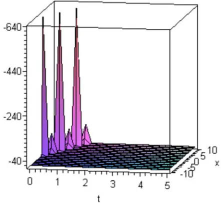
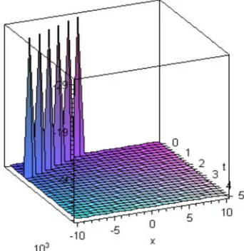
From graphical representations, we note that soliton is a wave which preserves its shape after it has collided with another wave of the same kind. By solving nonlinear evolution equations included foam drainage equation and fourth order evolution equation, we attain desired solitary wave solutions for different values of random parameters. The solitary wave moves toward right if the velocity is positive. It turns in left directions if the velocity is negative. The amplitudes and velocities are controlled by various parameters. Figures signify graphical representation for different values of parameters. Figure 1 to 11 represents periodic wave solution for different values of parameters ^, V and µ. The soliton solutions that are shown in figure 12 to 15 and figure 17 to 20 represents solitary wave solutions for different values of parameters V and µ. Figure 16 shows peakons solution by using values of parameters as V 4, μ 2. In all cases, for various values of parameters, we attain identical solitary wave solutions which obviously show that the final solution is not effectively based upon these parameters. So, we can choose arbitrary values of such parameters as input to our simulations.

5. Conclusion

(11)

computational work, and the graphical representations. Results obtained by this method are very encouraging and reliable for solving any other type of NLEEs. The graphical representations clearly indicate the solitary solutions.

References

[1] I. Aslan, Exact and explicit solutions to some nonlinear evolution equations by utilizing the (G’/G)-expansion method, App. Math. Comp., 217 (20), 8134-8139, 2011.

[2] A. Bekir, Application of the (G’/G)-expansion method for nonlinear evolution equations. Phys. Lett. A 372, 3400–3406, 2008.

[3] M. F. El-Sabbagh, A. T. Ali, and S. El-Ganaini, New Abundant Exact Solutions for the System of (2+1)-Dimensional Burgers Equations, App. Math. Inf. Sci., 2 (1), 31-41, 2008.

[4] J. Feng, W. Li and Q. Wan, “Using (G′/G)−expansion method to seek traveling wave solution of

Kolmogorov-Petrovskii-Piskunov equation,” App. Math. Comput., 217, 5860-5865, 2011.

[5] K. A. Gepreel, “Exact solutions for nonlinear PDEs with the variable coefficients in mathematical physics,” J. Inf. Comput. Sci., 6 (1), 003-014, 2011.

[6] F. Khanib, S. H. Nezhad, M. T. Darvishia, S. W. Ryu, New solitary wave and periodic solutions of the foam drainage equation using the Exp-function method, Nonlinear Analysis, Real World App., 10, 1904–1911, 2009.

[7] X. Liu, L. Tian, Y. Wu, Application of (G`/G)-expansion method to two nonlinear evolution equations. Appl. Math. Comput., in press, (2009).

[8] H. Naher, F. Abdullah and M. A. Akbar, “The (G′/G)−expansion method for abundant traveling wave solutions of Caudrey-Dodd-Gibbon equation,” Mathematical Problems in Engineering, 2011, 218216, (in press), 2011. [9] T. Ozis and I. Aslan, “Application of the (G′/G)−expansion

method to Kawahara type equations using symbolic computation,” App. Math. Comput., 216, 2360-2365, 2010. [10] I. Podlubny, Geometric and Physical Interpretation of

Fractional Integration and Fractional Differentiation, fract. Cal. App. anal., 5, Number 4, 2002.

[11] A. M. Wazwaz, Solitary wave solutions and periodic solutions, for higher-order nonlinear evolution equations, App. Math. Comput., 181, 1683–1692, 2006.

[12] M. Wang, X. Li and J. Zhang, The (G′/G)−expansion method and traveling wave solutions of nonlinear evolution equations in mathematical physics, Phy. Lett. A, 372, 417-423, 2008. [13] A. Yildirim and S. T. Mohyud-Din, Analytical approach to

space and time fractional Burger’s equations, Chinese Phy. Lett., 27 (9), 090501, 2010.

[14] E. M. E. Zayed, and S. Al-Joudi, “Applications of an Extended (G′/G)−Expansion Method to Find Exact Solutions of Nonlinear PDEs in Mathematical Physics,” Math, Prob. Eng., 768573, 2010.

[15] Q. M. Hassan and S. T. Mohyud-Din, Investigating biological population model using exp-function method. Int. J. Biomath. 9 (2), 1650026, 2016.

[16] Duranda M, Langevin D. Physicochemical approach to the theory of foam drainage. Europhys J Eng., 7:35-44, 2002. [17] Y. M. Zhao, Y. J. Yang and W. Li, “Application of the improved

(G′/G)−expansion method for the Variant Boussinesq equations,” App. Math. Sci., 5 (58), 2855-2861, 2011. [18] E. M. E. Zayed and M. A. M. Abdelaziz, An extended (G′/G) −

expansion method and its applications to the (2+1)-dimensional nonlinear evolution equations, Wseas Transactions on Mathematics, 11 (11), 1039-1047, 2012.

[19] J. Chen and B. Li, Multiple (G`/G)-expansion method and its applications to nonlinear evolution equations in mathematical physics, Ind. Acad. Sci., 28 (3), 375-388, 2012.

[20] M. Wang, J. Zhang and X. Li, Application of the (G′/G) expansion to traveling wave solutions of the Broer-Kaup and the approximate long water wave equations. Appl. Math. Comput., 206, 321-326, 2008. Oz ̈is

[21] I. Aslan and T. Oz ̈is, Analytic study on two nonlinear evolution equations by using the (G`/G)-expansion method. Appl. Math. Comput. 209, 425-429, 2009.

[22] X. J. Yang, A new integral transform operator for solving the heat-diffusion problem, Applied Mathematics Letters. 64 (2017) 193-197.

[23] X. J. Yang, A New integral transform method for solving steady Heat transfer problem, Thermal Science. 20 (2016) S639-S642.

[24] X. J. Yang, J. A. Tenreiro Machado, D. Baleanu, C. Cattani, On exact traveling wave solutions for local fractional Korteweg-de Vries equation, Chaos. 26 (8) (2016) 084312.

[25] X. J. Yang, G. Feng, H. M. Srivastava, Exact travelling wave solutions for the local fractional two-dimensional Burgers-type equations, Computers & Mathematics with Applications. 73 (2) (2017) 203-210.

[26] X. J. Yang, J. A. Tenreiro Machado, D. Baleanu, On exact traveling-wave solution for local fractional Boussinesq equation in fractal domain, Fractals. 25 (4) (2017) 1740006. [27] X. J. Yang, G. Feng, H. M. Srivastava, Non-Differentiable

exact solutions for the nonlinear ODEs defined on fractal sets, Fractals. 25 (4) (2017) 1740002.

[28] K. M. Saad, E. H. AL-Shareef, M. S. Mohamed, X. J. Yang, Optimal q-homotopy analysis method for time-space fractional gas dynamics equation, The European Physical Journal Plus. 132 (23) (2017)https://doi.org/10.1140/epjp/i2017-11303-6. [29] X. J. Yang, G. Feng, A New Technology for Solving Diffusion