R E S E A R C H
Open Access
Greedy low-rank algorithm for spatial
connectome regression
Patrick Kürschner
1, Sergey Dolgov
2, Kameron Decker Harris
3and Peter Benner
4**Correspondence:
[email protected] 4Computational Methods in
Systems and Control Theory, Max Planck Institute for Dynamics of Complex Technical Systems, Magdeburg, Germany Full list of author information is available at the end of the article
Abstract
Recovering brain connectivity from tract tracing data is an important computational problem in the neurosciences. Mesoscopic connectome reconstruction was
previously formulated as a structured matrix regression problem (Harris et al. in Neural Information Processing Systems,2016), but existing techniques do not scale to the whole-brain setting. The corresponding matrix equation is challenging to solve due to large scale, ill-conditioning, and a general form that lacks a convergent splitting. We propose a greedy low-rank algorithm for the connectome reconstruction problem in very high dimensions. The algorithm approximates the solution by a sequence of rank-one updates which exploit the sparse and positive definite problem structure. This algorithm was described previously (Kressner and Sirkovi´c in Numer Lin Alg Appl 22(3):564–583,2015) but never implemented for this connectome problem, leading to a number of challenges. We have had to design judicious stopping criteria and employ efficient solvers for the three main sub-problems of the algorithm, including an efficient GPU implementation that alleviates the main bottleneck for large datasets. The performance of the method is evaluated on three examples: an artificial “toy” dataset and two whole-cortex instances using data from the Allen Mouse Brain Connectivity Atlas. We find that the method is significantly faster than previous methods and that moderate ranks offer a good approximation. This speedup allows for the estimation of increasingly large-scale connectomes across taxa as these data become available from tracing experiments. The data and code are available online.
Keywords: Matrix equations; Computational neuroscience; Low-rank approximation; Networks
1 Introduction
Neuroscience and machine learning are now enjoying a shared moment of intense inter-est and exciting progress. Many computational neuroscientists find themselves inspired by unprecedented datasets to develop innovative methods of analysis. Exciting examples of such next-generation experimental methodology and datasets are large-scale record-ings and precise manipulations of brain activity, genetic atlases, and neuronal network tracing efforts. Thus, techniques which summarize many experiments into an estimate of the overall brain network are increasingly important. Many believe that uncovering such network structures will help us unlock the principles underlying neural computation and brain disorders (Grillner et al. [17]). Initial versions of such connectomes (Knox et al. [25]) are already being integrated into large-scale modeling projects (Reimann et al. [40]).
We present a method which allows us to perform these reconstructions faster, for larger datasets.
Structural connectivity refers to the synaptic connections formed between axons (out-puts) and dendrites (in(out-puts) of neurons, which allow them to communicate chemically and electrically. We represent such networks as a weighted, directed graph encoded by a nonnegative adjacency matrixW. The network of whole-brain connections orconnectome is currently studied at a number of scales (Sporns [46], Kennedy et al. [24]): Microscopic connectivity catalogues individual neuron connections but currently is restricted to small volumes due to difficult tracing of convoluted geometries (Kasthuri et al. [23]). Macro-scopic connectivity refers to connections between larger brain regions and is currently known for a number of model organisms (Buckner and Margulies [7]). Mesoscopic con-nectivity (Mitra [32]) lies between these two extremes and captures projection patterns of groups of hundreds to thousands of neurons among the 106–1010neurons in a typical mammalian brain.
Building on previous work (Harris et al. [19]; Knox et al. [25]), we present a scalable method to infer spatially-resolved mesoscopic connectome from tracing data. We apply our method to data from the Allen Mouse Brain Connectivity Atlas (Oh et al. [34]) to reconstruct mouse cortical connectivity. This resource is one of the most comprehensive publicly available datasets, but similar data are being collected for fly (Jenett et al. [22]), rat (Bota et al. [6]), and marmoset (Majka et al. [30]), among others. Our focus is on present-ing and profilpresent-ing an improved algorithm for connectome inference. By developpresent-ing scalable methods as in this work, we hope to enable the reconstruction of high-resolution connec-tomes in these diverse organisms.
1.1 Mathematical formulation of a spatial connectome regression problem
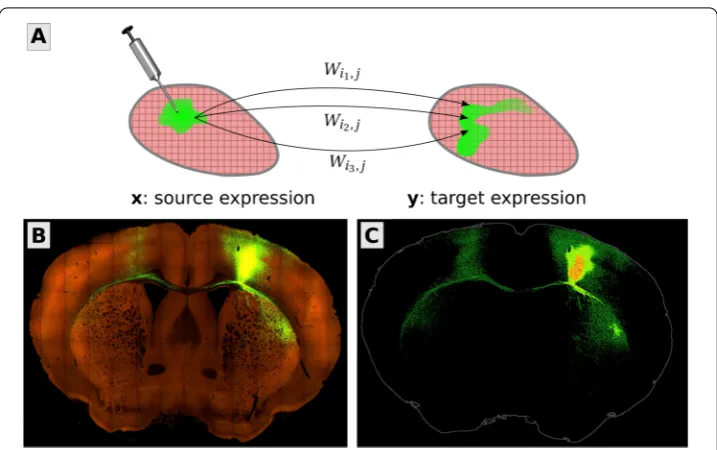
We focus on the mesoscale because it is naturally captured by viral tracing experiments (Fig.1). In these experiments, a virus is injected into a specific location in the brain, where it loads the cells with proteins that can then be imaged, tracing out the projections of those neurons with cell bodies located in the injection site. The source and target signals, within and outside of the injection sites, are measured as the fraction of fluorescing pixels within cubic voxels. These form the data matricesX∈RnX×ninjandY∈RnY×ninj, where
parame-tersnXandnYare the number of locations in the discretized source and target regions of thed-D brain, andninjis the number of injections. In general,nXandnYmay be unequal, e.g. if injections were only delivered to the right hemisphere of the brain. Each experiment only traces out the projections from that particular injection site. By performing many such experiments, with multiple mice, and varying the injection sites to cover the brain, one can then “stitch” together a mesoscopic connectome for the average mouse. We refer the interested reader to (Oh et al. [34]) for more details of the experimental procedures.
We present a new low-rank approach to solving the smoothness-regularized optimiza-tion problem posed by Harris et al. [19]. Specifically, they considered solving the regular-ized least-squares problem
W∗=arg min
W≥0 1
2PΩ(WX–Y) 2
F
loss
+λ
2LyW+WL
x
2
F
regularization
Figure 1In this paper, we present an improved method for the mesoscale connectome inference problem. (A) The goal is to find a voxel-by-voxel matrixWso that the pattern of neural projectionsyarising from an injectionxis reproduced by matrix-vector multiplication,y≈Wx. The vectorsxandycontain the fraction of fluorescing pixels in each voxel from viral tracing experiments. (B) An example of the data, in this case a coronal slice from a tracing experiment delivered to primary motor cortex (MOp). Bright green areas are neural cells expressing the green fluorescent protein. (C) The raw data are preprocessed to separate the injection site (red/orange) from its projections (green). Fluorescence values in the injection site enter into the source vectorx, whereas fluorescence everywhere else is stored in the entries of the target vectory. Thexand
yare discretized volume images of the brain reshaped into vector form. EntryWijmodels the expected fluorescence at locationifrom one unit of source fluorescence at locationj, a linear operator mapping from source images to target images. Image credit (B and C): Allen Institute for Brain Science
where the minimum is taken over nonnegative matrices. The operator PΩ defines an entry-wise product (Hadamard product)PΩ(M) =M◦Ω, for any matrixM∈RnY×ninj,
andΩis a binary matrix, of the same size, which masks out the injection sites where the entries ofYare unknown.aWe take the smoothing matricesL
y∈RnY×nYandLx∈RnX×nX
to be discrete Laplace operator, i.e. the graph Laplacians of the voxel face adjacency graphs for discretized source and target regions. We choose a regularization parameterλ¯and set λ=λ¯nninj
X to avoid dependence onnX,nYandninj, since the loss term is a sum overnY×ninj
entries and the regularization sums overnY×nXmany entries.
1.2 Previous methods of mesoscale connectome regression
Much of the work on mesoscale mouse connectomes leverages the data and processing pipelines of the Allen Mouse Brain Connectivity Atlas available at http://connectivity. brain-map.org(Lein et al. [28]; Oh et al. [34]). In the early examples of such work, Oh et al. [34] used viral tracing data to construct regional connectivity matrices. Nonnega-tive matrix regression was used to estimate the regional connectivity. First, the injection data were processed into a pair of matricesXRegandYRegcontaining the regionalized in-jection volumes and proin-jection volumes, respectively. The rows of these matrices are the regions and the columns index injection experiments. Oh et al. [34] then used nonnega-tive least squares to fit a region-by-region matrixWRegsuch thatYReg≈WRegXReg. Due to numerical ill-conditioning and a lack of data, some regions were excluded from the analy-sis. Similar techniques have been used to estimate regional connectomes in other animals. Ypma and Bullmore [49] took a different approach, using a likelihood-based Markov chain Monte Carlo method to infer regional connectivity and weight uncertainty from the Allen data.
Harris et al. [19] made a conceptual and methodological leap when they presented a method to use such data for spatially-explicit mesoscopic connectivity. The Allen Mouse Brain Atlas is essentially a coordinate mapping which discretizes the average mouse brain into cubic voxels, where each voxel is assigned to a given region in a hierarchy of brain regions. They used an assumption of spatial smoothness to formulate (1), where the spe-cific smoothing term results in a high-dimensional thin plate spline fit (Wahba [48]). They then solved (1) using the generic quasi-Newton algorithm L-BFGS-B (Byrd et al. [8]). This technique was applied to the mouse visual areas but limited to small datasets sinceWwas dense. Using a simple low-rank version based on projected gradient descent, Harris et al. [19] argued that such a method could scale to larger brain areas. However, the initial low-rank implementation turned out to be too slow to converge for large-scale applications. Times to convergence were not reported in the original paper, but the full-rank version typically took around a day, while the low-rank version needed multiple days to reach a minimum.b
Knox et al. [25] simplified the mathematical problem by assuming that the injections were delivered to just a single voxel at the injection center of mass. Using a kernel smoother led to a method which is explicitly low-rank, with smoothing performed only in the in-jection space (columns ofW). This kernel method was applied to the whole mouse brain, yielding the first estimate of voxel–voxel whole-brain connectivity for this animal. How-ever, these assumptions do not hold in reality: The injections affect a volume of the brain that encompasses much more than the center of mass.cWe also expect that the connectiv-ity is also smooth across projection space (rows ofW), since the incoming projections to a voxel are strongly correlated with those of nearby voxels. These inaccuracies mean that the kernel method is prone to artifacts, in particular ones arising from the injection site locations, since there is no ability for that method to translate the source of projections smoothly away from injection sites. It is thus imperative to develop an efficient method for the spline problem that works for large datasets.
1.3 Continuous formulation motivates the need for sophisticated solvers
discrete version of an underlying continuous problem (similar to Rudin et al. [42], among others), where we define the cost as
1 2 ninj i=1
T∩Ωi S
W(x,y)Xi(x) dx–Yi(y) 2
dy+λ 2 T S
W(x,y)2dxdy. (2)
The cost is minimized overW:T×S→R, the continuous connectome, in an appropriate Sobolev space (square-integrable derivatives up to fourth order onT ×Sis sufficiently regular). The functionWmay be seen as the kernel of an integral operator fromStoT. These regions SandT are both compact subsets ofRdrepresenting source and target regions of the brain. The mask regionΩi⊂T is the subset of the brain excluding the
injection site. Finally, the discrete Laplacian termsLhave been replaced by the continuous Laplacian operatoronS×T. The parameterλagain sets the level of smoothing.d
For simplicity, considerS=T= the whole brain,Ωi=Tfor alli= 1, . . . ,ninjand relax the constraint of nonnegativity onW. Taking the first variational derivative of (2) and setting it to zero yields the Euler–Lagrange equations for this simplified problem:
0 =λ2W(x,y) –
ninj
i=1
Xi(x)Yi(y) +
S
Wx,y
ninj
i=1 Xi
xXi(x)
dx
=λ2W(x,y) –g(x,y) +
S
Wx,yfx,xdx, (3)
where for convenience we have defined the data covariance functions f(x,x) =
ninj
i=1Xi(x)Xi(x) and g(x,y) = ninj
i=1Xi(x)Yi(y), analogous to XXT andYXT. The
opera-tor2is the biharmonic operator or bi-Laplacian. Equation (3) is a fourth-order partial integro-differential equation in 2ddimensions.
Iterative solutions via gradient descent or quasi-Newton methods to biharmonic and similar equations can be slow to converge (Altas et al. [1]). It takes many iterations to prop-agate the highly local action of the biharmonic differential operator across global spatial scales due to the small stable step size (Rudin et al. [42]), whereas the integral part is inher-ently nonlocal. Very slow convergence is what we have found when applying methods like gradient descent to problem (1), also for low-rank versions. This includes quasi-Newton methods such as L-BFGS (Byrd et al. [8]). When we attempted to solve the whole-cortex top view and flatmap problems as in Sects.3.2and3.3, the method had not converged (from a naive initialization) after a week of computation. These difficulties motivated the development of the method we present here.
1.4 Outline of the paper
We present a greedy, low-rank algorithm tailored to the connectome inference problem. To leverage powerful linear methods, we consider solutions to the unconstrained problem
W∗=arg min
W
1
2PΩ(WX–Y) 2
F+
λ
2LyW+WL
x
2
F, (4)
computed solutionW∗to zero is adequate, or it can serve as an initial guess to an iterative solver for the slower nonnegative problem.
Equation (4) is another regularized least-squares problem. In Sect.2.1, we show that
taking the gradient and setting it equal to zero leads to a linear matrix equation in the unknownW. This takes the form of a generalized Sylvester equation with coefficient ma-trices formed from the data and Laplacian terms. The data mama-trices are, in fact, of low
rank sinceninjnX,nY, and thus we can expect a low-rank approximationW≈UVto the full solution to perform well (see Harris et al. [19], although we do not know how to justify this rigorously). We provide a brief survey of some low-rank methods for linear matrix equations in Sect.2.2. We employ a greedy solver that finds rank-one components
uivi one at a time, explained in Sect.2.3. After a new component is found, it is
orthogo-nalized and a Galerkin refinement step is applied. This leads to Algorithm1, our complete method.
We then test the method on a few connectome fitting problems. First, in Sect.3.1, we test
on a fake “toy” connectome, where we know the truth. This is a test problem consisting of a 1-D brain with smooth connectivity (Harris et al. [19]). We find that the output of our algorithm converges to the true solution as the rank increases and as the stopping
tolerance decreases. Next, we present two benchmarks using real viral tracing data from the isocortices of mice, provided by the Allen Institute for Brain Science. In each case, we work with 2-D data in order to limit the problem size and because the cortex is a relatively flat, 2-D shape. It has also been argued that such a projection also denoises such data
(Van Essen [47]; Gămănuţ et al. [14]). In Sect.3.2, we work with data that are averaged directly over the superior-inferior axis to obtain a flattened cortex. We refer to this as the top viewprojection. In contrast, for Sect.3.3, the data are flattened by averaging along
curved streamlines of cortical depth. We call this theflatmapprojection.
Finally, Sect.4discusses the limitations of our method and directions for future research. Our data and code are described in Sect.5and freely available for anyone who would like to reproduce the results.
2 Greedy low-rank method
2.1 Linear matrix equation for the unknown connectivity
We now derive the equivalent of the “normal equations” for our problem. Denote the
ob-jective function (4) asJ(W), with decomposition
J(W) =Jloss(W) +Jreg(W) = 1
2PΩ(WX–Y) 2
F+
λ
2LyW+WL
x
2
F.
WritingJlossindexwise, we obtain (note thatΩ◦Ω=Ω)
Jloss= 1 2
n,ninj
i,α=1 Ωi,α
m
k=1
Wi,kXk,α–Yi,α
The derivative reads
∂Jloss ∂Wˆı,kˆ
=
n,ninj
i,α=1 Ωi,α
m
k=1
Wi,kXk,α–Yi,α
Xˆk,αδi,ˆı
=
ninj
α=1
Ωıˆ,αXkˆ,α
m
k=1
(Xk,αWıˆ,k–Xkˆ,αΩıˆ,αYˆı,α),
or in vector form
∂Jloss ∂vec(W)=
ninj
α=1
XαXα
⊗diag(Ωα)vec(W) –vec(Ω◦Y)X,
whereXαis theαth column ofXand likewise forΩ. Setting the derivative equal to zeros leads to the system of normal equations
Avec(W) =vec(Ω◦Y)X, (5)
wherevec(W) is the vector of all columns ofWstacked on top of each other. This linear system features the following (nYnX)×(nYnX) matrix, consisting of ninj+ 3 Kronecker products,
A=
ninj
α=1
XαXα
⊗diag(Ωα) +λL2x⊗InY+ 2Lx⊗Ly+InX⊗L
2
y
. (6)
Note that without the observation mask,Ωis a matrix of all ones, and the first term com-presses toXX⊗InY.
The linear system (5) can be recast as the linear matrix equation
A(W) =D, (7)
with the operatorA(W) :=λB(W) +C(W), where
B(W) :=WL2x+ 2LyWLx+L2yW,
C(W) :=
ninj
α=1
diag(Ωα)WXαXα, and D:= (Ω◦Y)X.
The smoothing termBcan be expressed as a squared standard Sylvester operatorB(W) = L(L(W)), whereL(W) :=LyW+WLx. The operatorLis the graph Laplacian operator on
the discretization ofT×S. Furthermore, the right hand sideDis a matrix of rankninj, since it is an outer product of two rankninjmatrices.
2.2 Numerical low-rank methods for linear matrix equations
mostninjnX,nY. It is often observed and theoretically shown (Grasedyck [16]; Benner and Breiten [3]; Jarlebring et al. [21]) that the solutions of large matrix equations with low-rank right hand sides exhibit rapidly decaying singular values. Hence, the solutionW is expected to have small numerical rank in the sense that few of its singular values are larger than machine precision or the experimental noise floor. Intuitively, since we also seek very smooth solutions, this also helps control the rank, since high frequency compo-nents tend to be associated with small singular values. This motivates us to approximate the solution of (7) by a low-rank approximationW≈UVwithU∈RnY×r,V∈RnX×rand
rmin(nX,nY). The low-rank factors are then typically computed by iterative methods which never form the approximationUVexplicitly.
Several low-rank methods for computingU,Vhave been proposed, starting from meth-ods for standard Sylvester equationsAX+XB=D(e.g. Benner [2]; Benner et al. [4]; Benner and Saak [5]; Simoncini [44]) and more recently for general linear matrix equations like (7) (Damm [13]; Benner and Breiten [3]; Shank et al. [43]; Ringh et al. [41]; Jarlebring et al. [21]; Powell et al. [39]). However, these methods are specialized and require the problem to have particular structures or properties (e.g.,B,Chave to form a convergent splitting ofA), which are not present in the problem at hand. The main structures present in (7) are positive definiteness and sparsity ofLx,Ly.
An approach that is applicable to the matrix equation (7) is a greedy method as pro-posed by Kressner and Sirković [26], which is based on successive rank-1 approximations of the error. Because this method is quite general, we tailored specific components of the algorithm to our problem. Three main challenges were overcome: First, we choose a sim-pler stopping criterion for the ALS routine. Second, specific solvers were chosen for the three main sub-problems of the algorithm, which maximizes its efficiency. Third, we de-veloped a GPU implementation of the Galerkin refinement, to make this bottleneck step more efficient. We advocate this method in the rest of the paper.
2.3 Description and application of the greedy low-rank solver
Here we briefly review the algorithm from (Kressner and Sirković [26]) and explain how it is specialized for our particular problem. Assume there is already an approximate solution Wj≈W∗of the linear matrix equationA(W) =D, equation (7), with solutionW∗. We will
improve our solution by an update of rank one:Wj+1=Wj+uj+1vj+1, whereuj+1∈RnYand vj+1∈RnX. The update vectorsuj+1,vj+1are computed by minimizing an error functional that we will soon define. Since the operatorAis positive definite, it induces theA-inner productX,YA=Tr(YA(X)) and theA-normYA:=√Y,YA. So we finduj+1,vj+1 by minimizing the squared error in theA-norm:
(uj+1,vj+1) =arg min
u,vW
∗–W
j–uv
2
A
=arg min
u,v Tr
W∗–Wj–uv
AW∗–Wj–uv
=arg min
u,v Tr
W∗–Wj–uv
D–A(Wj) –A
uv.
Discarding constant terms, noting thatX,YA=Y,XA, and settingRj=D–A(Wj) leads
to
(uj+1,vj+1) =arg min
u,v
uv,uvA– 2TruvRj
Notice that the rank-1 decompositionuvis not unique, because we can rescale the factors by any nonzero scalarcsuch that (uc)(v/c)represents the same matrix. This reflects the fact that the optimization problem (8) is not convex. However, it is convex in each of the factorsuandvseparately.
We obtain the updates uj+1, vj+1 via an alternating linear (ALS) scheme (Ortega and Rheinboldt [35]). Although we only consider low-rank approximations of matrices here, ALS methods are also used for computing low-rank approximations of higher order ten-sors by means of polyadic decompositions (e.g. Harshman [20]; Sorber et al. [45]). First, a fixedvis used in (8) and a minimizinguis computed which is in the next stage kept fixed and (8) is solved for a minimizingv. For a fixed vectorvwithv= 1 the minimizing problem is
ˆ
u=arg min
u
uv,uvA– 2TruvRj
=arg min
u
λuuvL2xv+ 2uLyu
vLxv
+uL2yu
+
ninj
α=1
udiag(Ωα)uvXαXαv
– 2uRjv
and, hence,uˆis obtained by solving the linear system of equations
ˆ
Auˆ=Rjv, Aˆ :=λ
vL2xvI+ 2Ly
vLxv
+L2y+
ninj
α=1
diag(Ωα)vXαXαv
. (9a)
The second half iteration starts from the fixedu=u/ˆ ˆuand tries to find a minimizingvˆ by solving
ˆ
Bvˆ=Rju,
ˆ
B:=λL2x+ 2Lx
uLyu
+uL2yuI+
ninj
α=1
udiag(Ωα)uXαXα
(9b)
which can be derived by similar steps. The linear systems (9a) and (9b) inherit the sparsity fromLx,LyandΩ. Therefore they can be solved by sparse direct or iterative methods. We
use a sparse direct solver for (9a), as this was faster than the alternatives. The coefficient matrixBˆin (9b) is the sum of a sparse (Laplacian terms) matrix and a low-rank (rankninj data terms) matrix. In this case, we solve (9b) using the Sherman–Morrison–Woodbury formula (Golub and Van Loan [15]) and a direct solver for the sparse inversion.
of δ= 0.1, corresponding to 2–4 ALS iterations, is sufficient in practice for the overall convergence of the algorithm.
The second stage of the method is a non-greedy Galerkin refinement of the low-rank fac-tors. Suppose a rankjapproximationWj=
j
i=1uivi ofWhas been already computed. Let
U∈RnY×jandV∈RnX×jhave orthonormal columns, spanning the spaces span{u
1, . . . ,uj}
and span{v1, . . . ,vj}, respectively. We compute a refined approximationUZVforZ∈Rj×j
by imposing the following condition onto the residual:
(Galerkin condition)
FindZso that AUZV–D ⊥ UZV∈RnY×nX,Z∈Rj×j.
This leads to the dense, square matrix equation inZof dimensionj≤rnX,nY:
λZVL2xV+ 2ULyU
ZVLxV
+UL2yUZ
+
ninj
α=1
Udiag(Ωα)UZVXαXαV
=UDV. (10)
Equation (10) is a projected version of (7) and inherits its structure including the positive definiteness of the operator which acts onZ. Instead of using a direct method to solve (10) (as in Kressner and Sirković [26]), we employ an iterative method similar to Powell et al. [39]. Due to the positive definiteness, the obvious method of choice is a dense, matrix-valued conjugate gradient method (CG). Moreover, we reduce the number of iterations significantly by taking the solution Zfrom the previous greedy step as an initial guess. The improved solutionWj+1=UZVyields a new residualRj+1=D–A(Wj+1) onto which the ALS scheme is applied to obtain the next rank-1 updates. The complete procedure is illustrated in Algorithm1.
This Galerkin refinement substantially improves the greedy approximation, leading to a faster convergence rate (Kressner and Sirković [26]). The ALS stage is primarily used to sketch the projection bases for the Galerkin solution, which justifies the limited number of ALS steps. Use of the Galerkin refinement in the low-rank decomposition literature can be traced back to the greedy approximation in the CP tensor format (Nouy [33]), as well as orthogonal matching pursuit approaches in sparse recovery and compressed sensing (Pati et al. [37]) and deflation strategies in low-rank matrix completion (Hardt and Wootters [18]).
3 Performance of the greedy low-rank solver on three problems
There are three test problems to which we apply Algorithm1: a toy problem with synthetic data (Sect.3.1), the top view projected mouse connectivity data (Sect.3.2), and the flatmap projected data (Sect.3.3). These tests show that the method easily scales to whole-brain connectome reconstruction.
We investigate the computational complexity and convergence of the greedy algorithm. Since the matrices in (9a) are sparse, the ALS steps needO(nr2n
Algorithm 1:Greedy rank-1 method with Galerkin projection for (7)
Input : MatricesLx,Ly,X,Ω,Y, maximal rankr≤min(nX,nY), tolerance 0 <τ1
Output: Low-rank approximation ofW=UZVin factored form
1 InitializeW0= 0,R0=D,U0=V0= [ ],j= 0
2 repeat
3 Pick initial vectorvfor ALS withv= 1, then get rank-1 update: 4 whileδ> 0.1 do
5 SolveAˆuˆ=Rjvforuˆ (sparse direct solver) and setu=u/ˆ ˆu Eq.(9a) 6 SolveBˆvˆ=Rjuforˆv(sparse direct + low-rank update)
7 and setv=v/ˆ ˆv Eq.(9b)
8 δ=|ˆˆuv– 1|
9 Uj+1= orth([Uj,u]),Vj+1= orth([Vj,v]) Orthogonalize new factors
10 Increment rankj←j+ 1
11 Solve Eq. (10) forZj(CG to toleranceτ/2) Galerkin update
12 Rj=D–A(UjZjVj) Update residual
13 δW=UjZjVj–Uj–1Zj–1Vj–1F/UjZjVjF
14 untilj=r orδW≤τ
investigate the cost in terms of the total computation time and the corresponding solution accuracy for a range of solution rank values.
The numerical experiments were performed on an Intel® E5-2650 v2 CPU with 8 threads and 64 Gb RAM. We employ an Nvidia® P100 GPU card for some subtasks: The Galerkin update relies on dense linear algebra to solve (10) by the CG method, so this stage admits an efficient GPU implementation. Algorithm1is implemented in MATLAB® R2017b, and was run on the Balena High Performance Computing Service at the University of Bath. See Sect.5for additional data and code resources.
We measure errors in the solution using the root mean squared error. Given any refer-ence solutionWof sizenY×nX, e.g. the truth or a large-rank solution when the truth is unknown, and a low-rank solution Wr, the RMS error is computed asE(Wr,W) =
W√r–WF
nYnX . We also report the relative error in the Frobenius normErel(Wr,W) =
Wr–WF WF .
3.1 Test problem: a toy brain
We use the same test problem as in Harris et al. [19], a one-dimensional “toy brain.” The source and target space areS=T= [0, 1]. The true connectivity kernel corresponds to a Gaussian profile about the diagonal plus an off-diagonal bump:
Wtrue(x,y) =e–(
x–y
0.4)2+ 0.9e–
(x–0.8)2+(y–0.1)2
(0.2)2 . (11)
The input and output spaces were discretized usingnX=nY= 200 uniform lattice points. Injections are delivered atninj= 5 locations inS, with a width of 0.12 + 0.1, where∼ Uniform(0, 1). The values ofXare set to 1 within the injection region and 0 elsewhere, Ωij= 1 –Xij,Y is set to 0 within the injection region, and we add Gaussian noise with
standard deviationσ= 0.1. The matricesLx=Lyare the 3-point graph Laplacians for the
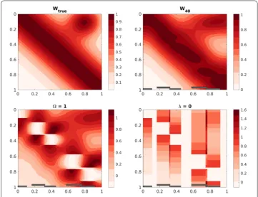
Figure 2Toy brain test problem. Top: true connectivity mapWtrue(left) and the low-rank solution with
rank= 40 andλ= 100 (right). Bottom: solutions withΩ= 1 (left) andλ= 0 (right). The locations of simulated injections are shown by the gray bars. This shows that both the mask (Ω) and the smoothing (λ> 0) are necessary for good recovery
Table 1 Computing times and errors for the toy brain test problem. The outputWis compared to
truth and a rank 140 reference solution
rank(W) 10 20 40 60 80
CPU time (sec.) 0.0396 0.1554 0.9653 2.6398 3.1108 E(W,W140) 3.2324e–01 5.5407e–02 1.4162e–02 1.2125e–03 3.1549e–04 E(W,Wtrue) 2.9418e–01 7.9921e–02 7.1537e–02 6.9777e–02 6.9821e–02 Erel(W,W140) 4.3320e–01 8.9700e–02 2.4900e–02 2.5000e–03 5.1300e–04 Erel(W,Wtrue) 4.0130e–01 1.1410e–01 1.0350e–01 1.0040e–01 1.0040e–01
We depict the true toy connectivityWtrue as well as a number of low-rank solutions output by our method in Fig.2. Both the mask and the regularization are required for good performance: If we remove the mask, settingΩequal to the matrix of all ones, then there are holes in the data at the location of the injections. If we try fitting withλ= 0, i.e. no smoothing, then the method cannot fill in holes or extrapolate outside the injection sites. It is only with the combination of all ingredients that we recover the true connectivity.
The computing time of the greedy method (in this example we use the CPU only version) remains in the order of seconds even for the largest considered ranks. In contrast, the unpreconditioned CG method needs thousands of iterations (and hundreds of seconds of time) to compute a solution within the same order of accuracy. Since it is unclear how to develop a preconditioner for Eq. (5), especially for a non-trivialΩ, in the next sections we focus only on the greedy algorithm.
3.2 Mouse cortex: top view connectivity
We next benchmark Algorithm1on mouse cortical data projected into a top–down view. See Sect.5for details about how we obtained these data. Here, the problem sizes arenY= 44,478 andnX= 22,377 and the number of injectionsninj= 126. We use the smoothing parameterλ¯= 106.
We run the low-rank solver with the target solution rank varying fromr= 125 to 1000. The stopping tolerancesτ were decreased geometrically from 10–3 forr= 125 to 10–6 forr= 1000. This delivers accurate but cheap solutions to the Galerkin system (10) while ensuring that the algorithm reached the target rank.
These low-rank solutions are compared to the full-rank solutionWfull with r=nX= 22,377 found by L-BFGS (Byrd et al. [8]), similar to Harris et al. [19], which used L-BFGS-B to deal with the nonnegativity constraint. Note that this full-rank algorithm was initialized from the output of the low-rank algorithm. This led to a significant speedup: The full-rank method, initialized naively, had not reached a similar value of the cost function (4) after a weekof computation, but this “warm start” allowed it to finish within hours.
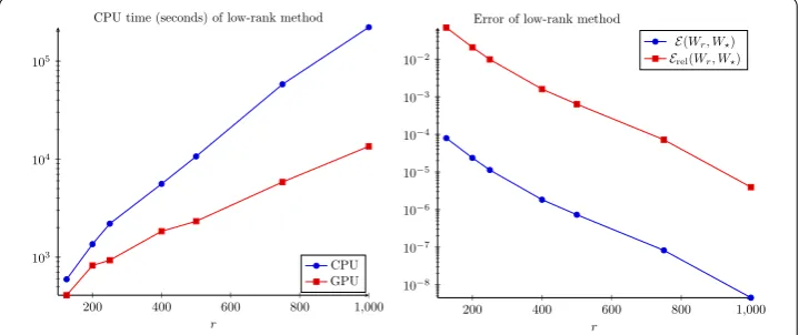
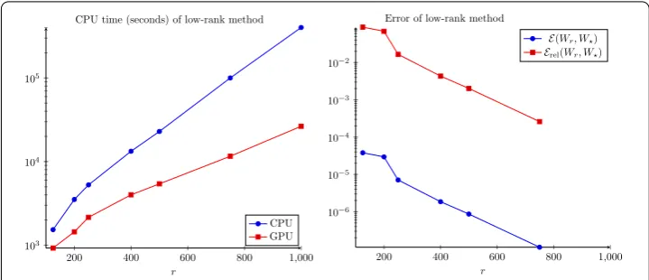
The computing times and errors are presented in Fig.3. We see that the RMS errors are relatively small for ranks above 500, below 10–6. Neither the RMS or relative error seem to have plateaued at rank 1000, but they are small. At rank 1000, the vector∞ er-ror (maximum absolute deviation of the matrices as vectors, not the matrix ∞-norm)
W1000–Wfull∞is less than 10–6, which is certainly within experimental uncertainty. In Fig.4, the value of the cost functionJ(Wr) is plotted against the rankrof the
approxima-tionWrfor the top view (left) and flatmap data (right). Apparently, aroundr= 500 the
cost function begins to stagnate indicating that the approximation quality does not signif-icantly improve any more. Hence, we continue the investigation with the numerical rank set tor= 500.
Figure 4Value of cost functionJ(Wr) versus the rankrof the low-rank approximationWr
We analyze the leading singular vectors of the solution. The output of the algorithm is Wr=UZV, which isnotthe SVD ofWrbecauseZis not diagonal. We perform a final
SVD of the Galerkin matrix,Z=UΣ˜ V˜and setUˆ =UU˜ andVˆ =VV˜, so thatWr=UΣˆ Vˆ
is the SVD of the solution.
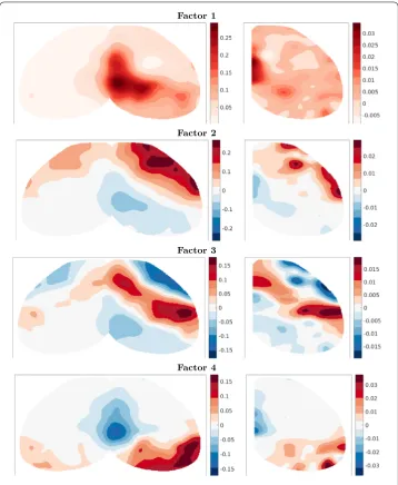
The first four of these singular vectors are shown in Fig.5. The brain is oriented with the medial-lateral axis aligned left–right and anterior–posterior axis aligned top–bottom, as in a transverse slice. The midline of the cortex is in the center of the target plots, whereas it is on the left edge of the source plots. We observe that the leading component is a strong projection from medial areas of the cortex near the midline to nearby locations. The second component provides a correction which adds local connectivity among posterior areas and anterior areas. Note that increased anterior connectivity arises from negative entries in both source and target vectors. The sign change along the roughly anterior– posterior axis manifests as a reduction in connectivity from anterior to posterior regions as well as from posterior to anterior regions. The third component is a strong local connec-tivity among somatomotor areas located medially along the anterior–posterior axis and stronger on the lateral side where the barrel fields, important sensory areas for whisking, are located. Finally, the fourth component is concentrated in posterior locations, mostly corresponding to the visual areas, as well as more anterior and medial locations in the retrosplenial cortex (thought to be a memory and association area). The visual and retro-splenial parts of the component show opposite signs, reflecting stronger local connectivity within these regions than distal connectivity between them.
These patterns in Fig.5are reasonable, since connectivity in the brain is dominantly local with some specific long-range projections. We also observe that the projection patterns (left componentsUΣ) are fairly symmetric across the midline. This is also expected dueˆ to the mirroring of major brain areas in both hemispheres, despite the evidence for some lateralization, especially in humans. The more specific projections between brain regions will show up in later, higher frequency components. However, it becomes increasingly difficult to interpret lower energy components as specific pathways, since these combine in complicated ways.
3.3 Mouse cortex: flatmap connectivity
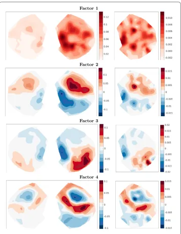
Figure 5Top four singular vectors of the top view connectivity withr= 500. Left: scaled target vectorsUˆΣ. Right: source vectorsVˆ
are missing from the top view since they curl underneath that vantage point. The flatmap is closer to the kind of transformation used by cartographers to flatten the globe, whereas the top view is like a satellite image taken far from the globe.
The problem size is now larger by roughly a factor of three relative to the top view. Here,nY= 126,847 andnX= 63,435. The number of experiments is the same,ninj= 126, whereas the regularization parameter is set toλ¯= 3×10⁷. The smoothing parameter was set to give the same level of smoothness, measured “by eye,” in the components as in the top view experiment. The tolerancesτ were as in the top view case.
Figure 6Computing times and errors for the flatmap data. The errors are computed with reference to the rank-1000 solutionW=W1000
significant than for the top view case. We obtained the rank 500 solution in approximately 1.5 hours, which is significantly less than with the pure CPU implementation, which took 6.4 hours. Comparing Figs.3and6, the computation times for the flatmap problem with r= 500 and 1000 are roughly twice as large as for the top view problem. On the other hand, forr= 125 and 250, the compute times are about three times as long for flatmap versus top view. The observed scaling in compute time appears to be slightly slower thanO(n) in these tests. The growth rate of the computing time on the GPU is better than that of the CPU version since the matrix multiplications, which dominate the CPU cost for large ranks, are calculated in nearly constant time, mainly due to communication overhead, on the GPU. The RMS error between rank 500 and 1000 is again less than 10–6, so we believe rank 500 is probably a very good approximation to the full solution. Figure4(right) shows the costs versus the approximation rank. Again, we see thatr= 500 is reasonable and the distance fromWis smaller than 10%.
The four dominant singular vectors of the flatmap solution are shown in Fig.7, oriented as in Fig.5, with the anterior–posterior axis from top–bottom and the medial-lateral axis from left–right. The first two factors are directly comparable between the two problem outputs, although we see more structure in the flatmap components. This could be due to employing a projection which more accurately represents these 3-D data in 2-D, or due to the choice of smoothing parameterλ. The third and fourth components, on the¯ other hand, are comparable to the fourth and third components in the top view problem, respectively. Again, these patterns are reasonable and expected. The raw 3-D data that were fed into the top view and flatmap projections were the same, but the greedy algorithm is run using different projected datasets. It is reassuring that we can interpret the first few factors and directly compare them against those in the top view.
3.4 Dropping the nonnegativity constraint does not strongly affect the solutions
In order to apply linear methods, we relaxed the nonnegativity constraint when formulat-ing the unconstrained problem (4), as opposed to the original problem with nonnegativity constraint (1). We now show that the resulting solutions are not significantly different be-tween the two problems. This justifies the major simplification that we have made.
Figure 7Top four singular vectors of the flatmap connectivity withr= 500. Left: scaled target vectorsUˆΣ. Right: source vectorsVˆ
entries were all greater than –0.0023 in the lower-left corner of the matrix (see Fig.2), where the truth is approximately zero.
unconstrained problem is also close to the constrained solution. Algorithm1thus offers an efficient way to approximate the solution to the more difficult nonnegative problem, while retaining low rank.
4 Discussion
We have studied a numerical method specifically tailored for the important neuroscience problem of connectome regression from mesoscopic tract tracing experiments. This con-nectome inference problem was formulated as the regression problem (4). The optimality conditions for this problem turn out to be a linear matrix equation in the unknown con-nectivityW, which we propose to solve with Algorithm1. Our numerical results show that the low-rank greedy algorithm, as proposed by Kressner and Sirković [26], is a viable choice for acquiring low-rank factors ofWwith a computation cost that was significantly smaller compared to other approaches (Harris et al. [19]; Benner and Breiten [3]; Kressner and Tobler [27]). This allows us to infer the flatmap matrix, with approximately 140×more entries than previously obtained for the visual system, while taking significantly less time: computing the flatmap solution took hours versus days for the smaller low-rank visual net-work (Harris et al. [19]). The first few singular vector components of these cortical con-nectivities are interpretable and reasonable from a neuroanatomy standpoint, although a full anatomical study of this inferred connectivity is outside the scope of the current paper. The main ingredients of Algorithm1are solving the large, sparse linear systems of equa-tions at each ALS iteration and solving the dense but small projected version of the original linear matrix equation for the Galerkin step. We had to carefully choose the solvers for each of these phases of the algorithm. The Galerkin step forms the principal bottleneck due to the absence of direct numerical methods to handle dense linear matrix equations of moderate size. We employed a matrix-valued CG iteration to approximately solve (10), implementing it on the GPU for speed. This lead to cubic complexity inrat this step. One could argue that equipping this CG iteration with a preconditioner could speed up its con-vergence, but so far we were not successful in finding a preconditioner that both reduced the number of CG steps and the computational time. A future research direction could be to derive an adequate preconditioning strategy for the problem structure in (7), which would increase the efficiency of any Krylov method.
Matrix-valued Krylov subspace methods (Damm [13]; Kressner and Tobler [27]; Ben-ner and Breiten [3]; Palitta and Kürschner [36]) offer an alternative class of possible algo-rithms to solving the overall linear matrix equation (7). However, for rapid convergence of these methods we typically need a preconditioner. In our tests on (7), these approaches performed poorly, because rank truncations (e.g. via thin QR or SVD) are required after major subcalculations which occur at every iteration. Computing these decompositions quickly became expensive because of the sheer amount of necessary rank truncations in the Krylov method. If a suitable preconditioner for our problem would be found, it would make sense to give low-rank matrix-valued Krylov methods another try.
Working directly with nonnegative factorsU≥0 andV≥0 was originally proposed by Harris et al. [19], where they applied a projected gradient method to find such an approx-imation for connectome of mouse visual areas albeit very slowly. Such a formulation is preferred, since it leads to a nonnegativeW, and it allows interpreting the leading factors as the most important neural pathways in the brain. Modifying Algorithm1to compute nonnegative low-rank factors or enforcing that the low-rank approximationUV≈Wis nonnegative—a nonlinear constraint—is a much harder goal to achieve. For instance, even if one generated nonnegative factor matricesUandV, e.g. by changing the ALS step to nonnegative ALS, the orthogonalization and Galerkin update each destroy this nonnega-tivity. New methods of NMF which incorporate regularizations similar to our Laplacian terms (Cichocki et al. [12]; Cai et al. [9]) are an area of ongoing research, and the optimiza-tion techniques developed there could accelerate the nonnegative low-rank formulaoptimiza-tion of (1). These include other techniques developed with neuroscience in mind, such as neuron segmentation and calcium deconvolution (Pnevmatikakis et al. [38]) as well as sequence identification (Mackevicius et al. [29]). The greedy method we have presented is an excel-lent way to initialize the nonnegative version of the problem, similar to how SVD is used to initialize NMF. We hope to improve upon nonnegative low-rank methods in the future. Model (1) is certainly not the only approach to solving the connectome inference prob-lem. The loss termPΩ(WX–Y)2
F is standard and arises from Gaussian noise
assump-tions combined with missing data and is standard loss in matrix completion problems with noisy observations (e.g. Mazumder et al. [31]; Candes and Plan [10]). The regularization term is a thin plate spline penalty (Wahba [48]). This is one of many possible choices for smoothing, among them penalties such asgrad(W)2or the total variation semi-norm (Rudin et al. [42]; Chambolle and Pock [11]), which favors piecewise-constant solutions. While we recognize that there are many possible choices for the regularizer, the thin plate penalty is reasonable, linear and thus convenient to work with. Previous work (Harris et al. [19]) has shown that it is useful for the connectome problem. Testing other forms of reg-ularization is a worthy goal but not straightforward to implement at scale. This is outside the scope of the current paper.
Finally, the most exciting prospects for this class of algorithms is what can be learned when we apply them to next-generation tract tracing datasets. Such techniques can be used to resolve differences between the rat (Bota et al. [6]) brain and mouse (Oh et al. [34]), or uncover unknown topographies (see Reimann et al. [40]) in these and other ani-mals (like the marmoset, Majka et al. [30]). The mesoscale is also naturally the same res-olution as obtained by wide-field calcium imaging. Spatial connectome modeling could elucidate the largely mysterious interactions different sensory modalities, proprioception, and motor areas, hopefully leading to better understanding of integrative functions.
5 Data and code
We tested our algorithm on two datasets (top view and flatmap) generated from Allen Institute for Brain Science Mouse Connectivity Atlas data http://connectivity.brain -map.org. These data were obtained with the Python SDK allensdk version 0.13.1 available fromhttp://alleninstitute.github.io/AllenSDK/. Our data pulling and processing scripts are available fromhttps://github.com/kharris/allen-voxel-network.
using either the top view or flatmap paths and saved as 2-D arrays. Next, the projected co-ordinates were split into left and right hemispheres. Sincewildtypeinjections were always delivered into the right hemisphere, this becomes our source spaceSwhereas the union of left and right are the target spaceT. We constructed 2-D 5-point Laplacian matrices on these grids with “free” Neumann boundary conditions on the cortical edge. Finally, the 2-D projected data were downsampled 4 times along each dimension to obtain 40μm resolution. The injection and projection data were then stacked into the matricesXand Y, respectively. The maskΩwas set viaΩij= 1{Xij≤0.4}.
MATLAB code which implements our greedy low-rank algorithm (1) is included in the repository:https://gitlab.mpi-magdeburg.mpg.de/kuerschner/lowrank_connectome. We also include the problem inputsX,Y,Lx,Ly,Ωfor our three example problems (test, top
view, and flatmap) as MATLAB files. Note thatΩis stored as 1 –Ωin these files, as this matches the convention of (Harris et al. [19]).
Acknowledgements
We would like to thank Lydia Ng, Nathan Gouwens, Stefan Mihalas, Nile Graddis and others at the Allen Institute for the top view and flatmap paths and general help accessing the data. Thank you to Braden Brinkman for discussions of the continuous problem, to Stefan Mihalas and Eric Shea-Brown for general discussions. This work was primarily generated while PK was affiliated with the Max Planck Institute for Dynamics of Complex Technical Systems.
Funding
KDH was supported by the Big Data for Genomics and Neuroscience NIH training grant and a Washington Research Foundation Postdoctoral Fellowship. SD is thankful to the Engineering and Physical Sciences Research Council (UK) for supporting his postdoctoral position at the University of Bath through Fellowship EP/M019004/1, and the kind hospitality of the Erwin Schrödinger International Institute for Mathematics and Physics (ESI), where this manuscript was finalized during the Thematic ProgrammeNumerical Analysis of Complex PDE Models in the Sciences.
Abbreviations
MOp, primary motor cortex; L-BFGS, Limited-memory Broyden–Fletcher–Goldfarb–Shanno algorithm; L-BFGS-B, L-BFGS with Box constraints;d-D,d-dimensional; ALS, Alternating Linear Scheme; Eq., Equation; CG, Conjugate Gradient (method); CP, Canonical Polyadic (decomposition); GPU, Graphics Processing Unit; RMS, Root Mean Square (error); SVD, Singular Value Decomposition; NMF, Nonnegative Matrix Factorization.
Availability of data and materials
Links to data and code are provided in Sect.5.
Ethics approval and consent to participate
Not applicable.
Competing interests
The authors declare that they have no competing interests.
Consent for publication
Not applicable.
Authors’ contributions
PK, SD and PB developed the greedy algorithm and performed numerical experiments. KDH prepared the viral tracing data, implemented the L-BFGS algorithm and performed comparisons, plotting and analysis of results. All authors planned the project and wrote, read and approved the final manuscript.
Author details
1Department of Electrical Engineering ESAT/STADIUS, KU Leuven, Leuven, Belgium.2Department of Mathematical Sciences, University of Bath, Bath, UK.3Paul G. Allen School of Computer Science & Engineering, Biology, University of Washington, Seattle, USA.4Computational Methods in Systems and Control Theory, Max Planck Institute for Dynamics of Complex Technical Systems, Magdeburg, Germany.
Endnotes
a In this paper, we take a different convention forΩ(the complement) as in Harris et al. [19].
b KD Harris, personal communication, 2017. Note that these times are for the much smaller visual areas dataset. c Wildtype injections can cover 30–500 voxels, approximately 240 on average, at 100μm resolution (Oh et al. [34]). d One may consider rescalingλas before, but subtle differences arise. In the continuous versus discrete cases the
units of the equations are different, since the functionsXi(x) andYi(y) are now viewed as densities. Furthermore,
operator is not. This explains the lack of any dependence on the grid size in the scaling of the discrete problem. Regardless, choosing the exact scaling to make the continuous and discrete cases match is not necessary for the more qualitative argument we are making.
Publisher’s Note
Springer Nature remains neutral with regard to jurisdictional claims in published maps and institutional affiliations.
Received: 18 April 2019 Accepted: 30 October 2019
References
1. Altas I, Dym J, Gupta M, Manohar R. Multigrid solution of automatically generated high-order discretizations for the biharmonic equation. SIAM J Sci Comput. 1998;19(5):1575–85.https://doi.org/10.1137/S1464827596296970. 2. Benner P. Solving large-scale control problems. IEEE Control Syst Mag. 2004;14(1):44–59.
3. Benner P, Breiten T. Low rank methods for a class of generalized Lyapunov equations and related issues. Numer Math. 2013;124(3):441–70.https://doi.org/10.1007/s00211-013-0521-0.
4. Benner P, Li R-C, Truhar N. On the ADI method for Sylvester equations. J Comput Appl Math. 2009;233(4):1035–45. 5. Benner P, Saak J. Numerical solution of large and sparse continuous time algebraic matrix Riccati and Lyapunov
equations: a state of the art survey. GAMM-Mitt. 2013;36(1):32–52.https://doi.org/10.1002/gamm.201310003. 6. Bota M, Dong H-W, Swanson LW. From gene networks to brain networks. Nat Neurosci. 2003;6(8):795–9.
https://doi.org/10.1038/nn1096.
7. Buckner RL, Margulies DS. Macroscale cortical organization and a default-like apex transmodal network in the marmoset monkey. Nat Commun. 2019;10(1):1976.https://doi.org/10.1038/s41467-019-09812-8.
8. Byrd R, Lu P, Nocedal J, Zhu C. A limited memory algorithm for bound constrained optimization. SIAM J Sci Comput. 1995;16(5):1190–208.https://doi.org/10.1137/0916069.
9. Cai D, He X, Han J, Huang TS. Graph regularized nonnegative matrix factorization for data representation. IEEE Trans Pattern Anal Mach Intell. 2011;33(8):1548–60.https://doi.org/10.1109/TPAMI.2010.231.
10. Candes EJ, Plan Y. Matrix completion with noise. Proc IEEE. 2010;98(6):925–36.
https://doi.org/10.1109/JPROC.2009.2035722.
11. Chambolle A, Pock T. An introduction to continuous optimization for imaging. Acta Numer. 2016;25:161–319.
https://doi.org/10.1017/S096249291600009X.
12. Cichocki A, Zdunek R, Huy Phan A, Amari S. Nonnegative matrix and tensor factorizations: applications to exploratory multi-way data analysis and blind source separation. New York: Wiley; 2009.
13. Damm T. Direct methods and ADI-preconditioned Krylov subspace methods for generalized Lyapunov equations. Numer Linear Algebra Appl. 2008;15(9):853–71.
14. G˘am˘anu¸t R, Kennedy H, Toroczkai Z, Ercsey-Ravasz M, Van Essen DC, Knoblauch K, Burkhalter A. The mouse cortical connectome, characterized by an ultra-dense cortical graph, maintains specificity by distinct connectivity profiles. Neuron. 2018;97(3):698–715.e10.https://doi.org/10.1016/j.neuron.2017.12.037.
15. Golub GH, Van Loan CF. Matrix computations. 4th ed. Baltimore: Johns Hopkins University Press; 2013.
16. Grasedyck L. Existence of a low rank orH-matrix approximant to the solution of a Sylvester equation. Numer Linear Algebra Appl. 2004;11:371–89.
17. Grillner S, Ip N, Koch C, Koroshetz W, Okano H, Polachek M, Poo M, Sejnowski TJ. Worldwide initiatives to advance brain research. Nat Neurosci. 2016.https://doi.org/10.1038/nn.4371.
18. Hardt M, Wootters M. Fast matrix completion without the condition number. In: Proceedings of the 27th conference on learning theory, COLT 2014. Barcelona, Spain, June 13–15, 2014. 2014. p. 638–78.
19. Harris KD, Mihalas S, Shea-Brown E. High resolution neural connectivity from incomplete tracing data using nonnegative spline regression. In: Neural information processing systems. 2016.
20. Harshman R. Foundations of the PARAFAC procedure: models and conditions for an “explanatory” multi-modal factor analysis. UCLA Working Papers in Phonetics. 1970;16.
21. Jarlebring E, Mele G, Palitta D, Ringh E. Krylov methods for low-rank commuting generalized Sylvester equations. Numer Linear Algebra Appl. 2018.
22. Jenett A, Rubin GM, Ngo T-TB, Shepherd D, Murphy C, Dionne H, Pfeiffer BD, Cavallaro A, Hall D, Jeter J, Iyer N, Fetter D, Hausenfluck JH, Peng H, Trautman ET, Svirskas RR, Myers EW, Iwinski ZR, Aso Y, DePasquale GM, Enos A, Hulamm P, Chun Benny Lam S, Li H-H, Laverty TR, Long Lei Qu F, Murphy SD, Rokicki K, Safford T, Shaw K, Simpson JH, Sowell A, Tae S, Yu Y, Zugates CT. A GAL4-driver line resource for drosophila neurobiology. Cell Reports. 2012;2(4):991–1001.
https://doi.org/10.1016/j.celrep.2012.09.011.
23. Kasthuri N, Hayworth KJ, Berger DR, Lee Schalek R, Conchello JA, Knowles-Barley S, Lee D, Vázquez-Reina A, Kaynig V, Jones TR, Roberts M, Lyskowski Morgan J, Carlos Tapia J, Sebastian Seung H, Gray Roncal W, Tzvi Vogelstein J, Burns R, Lewis Sussman D, Priebe CE, Pfister H, Lichtman JW. Saturated reconstruction of a volume of neocortex. Cell. 2015;162(3):648–61.https://doi.org/10.1016/j.cell.2015.06.054.
24. Kennedy H, Van Essen DC, Christen Y, editors. Micro-, meso- and macro-connectomics of the brain. Research and perspectives in neurosciences. Berlin: Springer; 2016.
25. Knox JE, Decker Harris K, Graddis N, Whitesell JD, Zeng H, Harris JA, Shea-Brown E, Mihalas S. High Resolution Data-Driven Model of the Mouse Connectome. bioRxiv 2018. p. 293019.https://doi.org/10.1101/293019.
26. Kressner D, Sirkovi´c P. Truncated low-rank methods for solving general linear matrix equations. Numer Linear Algebra Appl. 2015;22(3):564–83.https://doi.org/10.1002/nla.1973.
27. Kressner D, Tobler C. Krylov subspace methods for linear systems with tensor product structure. SIAM J Matrix Anal Appl. 2010;31(4):1688–714.
Jeung DP, Johnson RA, Karr PT, Kawal R, Kidney JM, Knapik RH, Kuan CL, Lake JH, Laramee AR, Larsen KD, Lau C, Lemon TA, Liang AJ, Liu Y, Luong LT, Michaels J, Morgan JJ, Morgan RJ, Mortrud MT, Mosqueda NF, Ng LL, Ng R, Orta GJ, Overly CC, Pak TH, Parry SE, Pathak SD, Pearson OC, Puchalski RB, Riley ZL, Rockett HR, Rowland SA, Royall JJ, Ruiz MJ, Sarno NR, Schaffnit K, Shapovalova NV, Sivisay T, Slaughterbeck CR, Smith SC, Smith KA, Smith BI, Sodt AJ, Stewart NN, Stumpf K-R, Sunkin SM, Sutram M, Tam A, Teemer CD, Thaller C, Thompson CL, Varnam LR, Visel A, Whitlock RM, Wohnoutka PE, Wolkey CK, Wong VY, Wood M, Yaylaoglu MB, Young RC, Youngstrom BL, Feng Yuan X, Zhang B, Zwingman TA, Jones AR. Genome-wide atlas of gene expression in the adult mouse brain. Nature.
2007;445(7124):168–76.https://doi.org/10.1038/nature05453.
29. Mackevicius EL, Bahle AH, Williams AH, Gu S, Denissenko NI, Goldman MS, Fee MS. Unsupervised Discovery of Temporal Sequences in High-Dimensional Datasets, with Applications to Neuroscience. bioRxiv 2018. p. 273128.
https://doi.org/10.1101/273128.
30. Majka P, Chaplin TA, Yu H-H, Tolpygo A, Mitra PP, Wójcik DK, Rosa MGP. Towards a comprehensive atlas of cortical connections in a primate brain: mapping tracer injection studies of the common marmoset into a reference digital template. J Comp Neurol. 2016;524(11):2161–81.https://doi.org/10.1002/cne.24023.
31. Mazumder R, Hastie T, Tibshirani R. Spectral regularization algorithms for learning large incomplete matrices. J Mach Learn Res. 2010;11:2287–322.
32. Mitra PP. The circuit architecture of whole brains at the mesoscopic scale. Neuron. 2014;83(6):1273–83.
https://doi.org/10.1016/j.neuron.2014.08.055.
33. Nouy A. Proper generalized decompositions and separated representations for the numerical solution of high dimensional stochastic problems. Arch Comput Methods Eng. 2010;17(4):403–34.
https://doi.org/10.1007/s11831-010-9054-1.
34. Oh SW, Harris JA, Ng L, Winslow B, Cain N, Mihalas S, Wang Q, Lau C, Kuan L, Henry AM, Mortrud MT, Ouellette B, Nghi Nguyen T, Sorensen SA, Slaughterbeck CR, Wakeman W, Li Y, Feng D, Ho A, Nicholas E, Hirokawa KE, Bohn P, Joines KM, Peng H, Hawrylycz MJ, Phillips JW, Hohmann JG, Wohnoutka P, Gerfen CR, Koch C, Bernard A, Dang C, Jones AR, Zeng H. A mesoscale connectome of the mouse brain. Nature. 2014;508(7495):207–14.
https://doi.org/10.1038/nature13186.
35. Ortega JM, Rheinboldt WC. Iterative solution of nonlinear equations in several variables. Philadelphia: SIAM; 2000. 36. Palitta D, Kürschner P. On the convergence of krylov methods with low-rank truncations. e-printarXiv:1909.01226
math.NA, 2019.
37. Pati YC, Rezaiifar R, Krishnaprasad PS. Orthogonal matching pursuit: recursive function approximation with applications to wavelet decomposition. In: Proceedings of 27th asilomar conference on signals, systems and computers. vol. 1. 1993. p. 40–4.https://doi.org/10.1109/ACSSC.1993.342465.
38. Pnevmatikakis EA, Soudry D, Gao Y, Machado TA, Merel J, Pfau D, Reardon T, Mu Y, Lacefield C, Yang W, Ahrens M, Bruno R, Jessell TM, Peterka DS, Yuste R, Paninski L. Simultaneous denoising, deconvolution, and demixing of calcium imaging data. Neuron. 2016;89(2):285–99.https://doi.org/10.1016/j.neuron.2015.11.037.
39. Powell CE, Silvester D, Simoncini V. An efficient reduced basis solver for stochastic Galerkin matrix equations. SIAM J Sci Comput. 2017;39(1):A141–63.https://doi.org/10.1137/15M1032399.
40. Reimann MW, Gevaert M, Shi Y, Lu H, Markram H, Muller E. A null model of the mouse whole-neocortex micro-connectome. Nat Commun. 2019;10(1):1–16.https://doi.org/10.1038/s41467-019-11630-x.
41. Ringh E, Mele G, Karlsson J, Jarlebring E. Sylvester-based preconditioning for the waveguide eigenvalue problem. Linear Algebra Appl. 2018;542:441–63.
42. Rudin LI, Osher S, Fatemi E. Nonlinear total variation based noise removal algorithms. Phys D: Nonlinear Phenom. 1992;60(1):259–68.https://doi.org/10.1016/0167-2789(92)90242-F.
43. Shank SD, Simoncini V, Szyld DB. Efficient low-rank solution of generalized Lyapunov equations. Numer Math. 2015;134:327–42.
44. Simoncini V. Computational methods for linear matrix equations. SIAM Rev. 2016;38(3):377–441.
45. Sorber L, Van Barel M, De Lathauwer L. Optimization-based algorithms for tensor decompositions: canonical polyadic decomposition, decomposition in rank-(Lr,Lr, 1) terms, and a new generalization. SIAM J Optim. 2013;23(2):695–720. https://doi.org/10.1137/120868323.
46. Sporns O. Networks of the brain. 1st ed. Cambridge: MIT Press. 2010. 47. Van Essen DC. Cartography and connectomes. Neuron. 2013;80(3):775–90.
https://doi.org/10.1016/j.neuron.2013.10.027.
48. Wahba G. Spline models for observational data. Philadelphia: SIAM; 1990.