R E S E A R C H
Open Access
Structure-based level set method for automatic
retinal vasculature segmentation
Bekir Dizdaro
ğ
lu
1,2*, Esra Ataer-Cansizoglu
2, Jayashree Kalpathy-Cramer
3, Katie Keck
4, Michael F Chiang
4,5and Deniz Erdogmus
2Abstract
Segmentation of vasculature in retinal fundus image by level set methods employing classical edge detection methodologies is a tedious task. In this study, a revised level set-based retinal vasculature segmentation approach is proposed. During preprocessing, intensity inhomogeneity on the green channel of input image is corrected by utilizing all image channels, generating more efficient results compared to methods utilizing only one (green) channel. A structure-based level set method employing a modified phase map is introduced to obtain accurate skeletonization and segmentation of the retinal vasculature. The seed points around vessels are selected and the level sets are initialized automatically. Furthermore, the proposed method introduces an improved zero-level contour regularization term which is more appropriate than the ones introduced by other methods for vasculature structures. We conducted the experiments on our own dataset, as well as two publicly available datasets. The results show that the proposed method segments retinal vessels accurately and its performance is comparable to state-of-the-art supervised/unsupervised segmentation techniques.
Keywords:Color retinal fundus images; Phase map; Segmentation of retinal vasculature; Structure and texture parts of retinal fundus image; Structure-based level set method
1 Introduction
Published ophthalmology studies reveal that there are often significant differences in clinical diagnosis of ret-inal diseases among medical experts [1]. Some of these approaches involve tedious processes. Manual segmenta-tion has become more and more time consuming with the increasing amount of patient data. An automatic retinal vasculature segmentation method may become an integral part of a computer-based image analysis and diagnosis sys-tems with improved accuracy and consistency [2].
Considering the conducted research, literature is full of examples [3-10] on vasculature segmentation, detec-tion, and other kinds of analysis employing especially su-pervised/unsupervised classification of pixels in retinal fundus images [11-19]. Marin et al. [14] and Soares et al. [15] presented two different supervised methods for segmentation of retinal vasculature by using moment
invariant-based features and 2-D Gabor filters, respectively. Staal et al. [16] proposed a retinal vasculature segmentation method using centerlines of a vessel base that are extracted by using image ridges. Budai et al. [17] presented an im-proved approach using Frangi’s method [18]. Other studies have employed centerline tracing methods and principal curves [19,20]. The reader may refer to [21] for more re-lated studies in the literature.
Level set-based methods have been widely used for image segmentation [22-34]. In general, these methods can be classified under two categories: (i) edge-based [22-30] and (ii) region-based [31-34] methods. However, level set-based methods have not been extensively employed in retinal vasculature segmentation. To the best of our knowledge, there have been only a few stud-ies in the literature proposing methods based on level sets to trace vasculature in retinal fundus images. This is due to challenges of vessel shapes in level set-based image segmentation methods [24]. Major challenges posed by the very thin and elongated structure of retinal vessels are further compounded by poor contrast in regions of interest for level set-based segmentation
* Correspondence:[email protected]
1
Department of Computer Engineering, Karadeniz Technical University, Trabzon 61080, Turkey
2
Cognitive Systems Laboratory, Northeastern University, Boston, MA 02115, USA
Full list of author information is available at the end of the article
methods. In one of those studies [24], the level set-based method is applied only on a selected region of images by implementing a non-automatic initialization of zero-level contours. These regions do not have any non-uniform intensity values. The method in [24] also employs edge information based on phase map and uses a re-initialization process to regularize the level set function, which is a problem in level set-based framework [25]. Moreover, this process requires complex discretization especially for re-initialization of the level set function. In addition, the method employs fixed filter coefficients to generate image features such as edges by using the log-Gabor filter, which does not generate a proper out-put to trace extremely thin retinal vessels in fundus im-ages smoothly. The level set segmentation method [26] proposed by Pang et al. requires the selection of initial contour in the form of long strips in the vertical direc-tion, and this is not an optimal selection. This selection leads to an increase in the number of iterations to gen-erate the results. According to the accuracy metric, the method produces poor results quantitatively on a non-pathological fundus image. Although they claim to present a fully automated method, the system requires mask images from the user. There are other level set ap-proaches [27-29,31-34] that focus on segmenting other vasculature structures in different image modalities such as ultrasound images and magnetic resonance im-ages (MRIs). However, these region-based methods [32,33] cannot be used extensively in segmentation of retinal fundus images due to the form of vascular struc-tures. Another method presented for retinal vessel seg-mentation [34] employs region-based level sets and region growing approaches, simultaneously.
In this paper, we present an improved and automatic level set-based method for retinal vasculature segmenta-tion. The presented method utilizes a robust phase map to determine image structures and seed points around the vessels in the initialization of the level set function. The performed tests on pathological and non-pathological fundus images demonstrate that the proposed method performs better than the existing approaches based on level sets.
The organization of the paper is structured as follows. ‘Section 2’ introduces the general information about retinal fundus images and level set-based methods developed for segmentation. ‘Section 3’ explains the proposed method and compares it with the existing ap-proaches in the literature. Experimental results are given in‘Section 4.’Finally,‘Section 5’presents a conclusion and possible future work in the field.
2 Background
LetI:Ω→ ℝ3be a color image defined on domainΩ→ ℝ2
, and let Ii: Ω→ ℝ represent the ith color channel of
the image I. Let p= (x, y) ∈ Ω, denote any point in Ω. Digital images have two additive components: structure part and texture part. These can be visualized as the car-toon version with sharp edges and noisy/textured ver-sion of the original image, respectively [35-37].
2.1 Characteristics of retinal fundus images
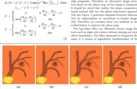
Retinal fundus images can be generated in color or gray-scale format in digital media. The pixels of a retinal fun-dus image are represented as color values in RGB color space as seen in Figure 1a,b. In terms of representation of retinal vessels, these images have mostly structure in-formation but also a texture part (noise, defects, etc.). The retinal fundus images can be split into two categor-ies, namely the pathological retinal fundus images and the non-pathological ones. The aim of segmentation methods for retinal fundus images is to separate vascula-tures from other regions as can be seen in Figure 1c,d. However, due to the structure of the optic disk and mac-ula, segmentation of blood vessels of retinal images is difficult. These regions have a more prominent intensity inhomogeneity compared to other parts of retinal im-ages. Furthermore, pathological images may contain de-fects and disorders such as drusen, geographic atrophy (GA), and non-uniform intensities. Such disorders also make the process of segmentation complicated.
As shown in Figure 2, each color channel inRGBcolor space can be separated and treated as an independent grayscale image. Considering those channels, the green channel component of the retinal image gives the best structure information to be processed [15,19] even though some regions such as the optic disk and macula in this channel component have non-uniform intensity levels. Let us use I instead of I2 to represent the green
channel component of the given image. In this case, the model would be as inI=bJ+ noise (defects) [33], where
bJand noise are considered as the structure component and the texture component, respectively. The green channel of the given image has some noises but no de-fects such as drusen, GA, etc.; the noise can be reduced using a convolution with a Gaussian filterGσof standard deviation σ. In the above equation, J is the true image, which consists of almost all constant values in an image region such as the optic disk, andbis referred to as the intensity inhomogeneity (shading artifact), which changes slowly throughout that image region.
2.2 Edge-based level set segmentation approach
Lipschitz continuous function Φ: Ω→ ℝ [22]. The level set evolution equation of the curve C with the speed function F is as given in Equation 1:
∂Φ
∂t ¼ Fðjj∇ΦjjÞ⋅ ð1Þ
Iterations of level set evolution are adversely affected by numerical errors and other factors that cause irregu-larities. Therefore, a frequent re-initialization process, formulated as ∂Φ/∂t= sign(Φ0) (1−||∇Φ||), could be
included to restore the regularity of the level set func-tion, establishing a stable level set evolution. Here, Φ0
is the level set function to be re-initialized and sign(.) stands for signum function. Re-initialization is per-formed by interrupting the evolution periodically and correcting irregularities of the level set function using a signed distance function. Even with a re-initialization process, in most of the level set methods such as the geodesic active counters (GAC) model [23], irregular-ities can still emerge [25]. Therefore, Li et al. intro-duced a new energy term called level set function regularization [25].
Image segmentation based on level set methods typic-ally consists of two additively combined energy terms, which are the length regularization term and the speed
Figure 2Color channel components of the non-pathological retinal fundus image presented in Figure 1b.Red(a), green(b), and blue (c)channel components.
Non-uniform intensities Optic disc
Macula
(b) (a)
(c) (d)
term related to the weighted area. The model is defined as E(Φ) =μR(Φ) +ϑL(Φ) +αA(Φ), where R(.), L(.), and
A(.) are the level set function regularization term, the
zero-level contour regularization term, and the term adjusting the speed of motion to zero-level contour, re-spectively. Here,μ, ϑ, andαare weighting parameters.
The level set function can be initialized in three differ-ent ways. In order to demonstrate the effect to the seg-mentation results, instead of a retinal fundus image, we employ a synthetic image that comprises artificially simi-lar vessels and defects (Figure 3).
1. Initialization with a signed distance function,d(.) (GAC model [23]) (Figure3a,b,c):
Φinitialð Þ ¼p
−dðp;CÞ in Ω0
0 onC
dðp;CÞ in ΩjΩ0
whereΩ0ðmarked by the
user or selected automaticallyÞ is an initial region inΩ:
8 < :
2. Initialization with a binary function (distance regularized level set evolution (DRLSE) model [25])
(Figure3a,d,e):Φinitial¼ −c0 inΩ0
c0 inΩjΩ0
, wherec0
is a small valued constant.
3. Initialization with a constant function (adaptive regularized level set (ARLS) model [28]) (Figure3f,g):
Φinitial=∓c0inΩ.
Edge-based level set methods have some drawbacks. Sometimes, a global minimum cannot be found and the methods tend to be slower than other segmentation methods. The global minimum can be correctly obtained if the initial contour is set properly. Level set-based methods also run faster when a narrow band approach is employed in the segmentation process.
3 The proposed method
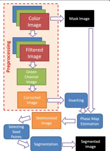
Our method can be considered in three main steps as outlined in Figure 4:
1. Preprocessing
2. Modified phase map estimation 3. Structure-based level set segmentation
More details about these steps are given in the follow-ing subsections of 3.1, 3.2, and 3.3.
3.1 Preprocessing for correction of non-uniform intensity A preprocessing step is employed for the correction of intensity inhomogeneity of retinal fundus images. Firstly, we apply a trace-based method to reduce noise and then a shock filter is applied to sharpen the image. Both filters work based on color information and give more robust results compared to the scalar approaches presented in [19,38]. Secondly, the green channel of the filtered image is extracted. Thirdly, two different images are generated by applying adaptive histogram equalization on the green channel image and then by applying a classical median filter on the equalized histogram image [19]. Lastly, depending on the case (intensity inhomogeneity),
one of the following is executed to produce the cor-rected image:
1. If the input image does not have intensity inhomogeneity, only the histogram-equalized green channel image in the previous step is taken into account as a corrected image. 2. Otherwise, the corrected image is produced by
division of those generated images.
To apply the trace-based method on color images, the local geometry for the color imageIis obtained by com-puting the fieldKof geometry tensors.Kis the gradient of I; K¼X3
i¼1∇Ii∇IiT; where∇Ii¼½∂Ii=∂x; ∂Ii=∂yT .
Moreover, K is expressed as the following for I in RGB
color space [39]:
K¼ k11 k12
k21 k22
¼ R2xþG 2 xþB
2
x RxRyþGxGyþBxBy
RyRxþGyGxþByBx R2yþG 2 yþB
2 y
;where
Rx¼∂I1=∂x; Gx¼∂I2=∂xandBx¼∂I3=∂x
Ry¼∂I1=∂y; Gy¼∂I2=∂yandBy ¼∂I3=∂y⋅
The positive eigenvaluesλ± and the orthogonal eigen-vectorsφ±ofKare calculated as
λ¼ k
11þk22
ffiffiffiffiffiffiffiffiffiffiffiffiffiffiffiffiffiffiffiffiffiffiffiffiffiffiffiffiffiffiffiffiffiffiffi k11−k22
ð Þ2þ
4k212 q
=2;and
φ¼
2k12 ; k22−k11
ffiffiffiffiffiffiffiffiffiffiffiffiffiffiffiffiffiffiffiffiffiffiffiffiffiffiffiffiffiffiffiffiffiffiffi k11−k22
ð Þ2þ
4k212 q
h iT
:
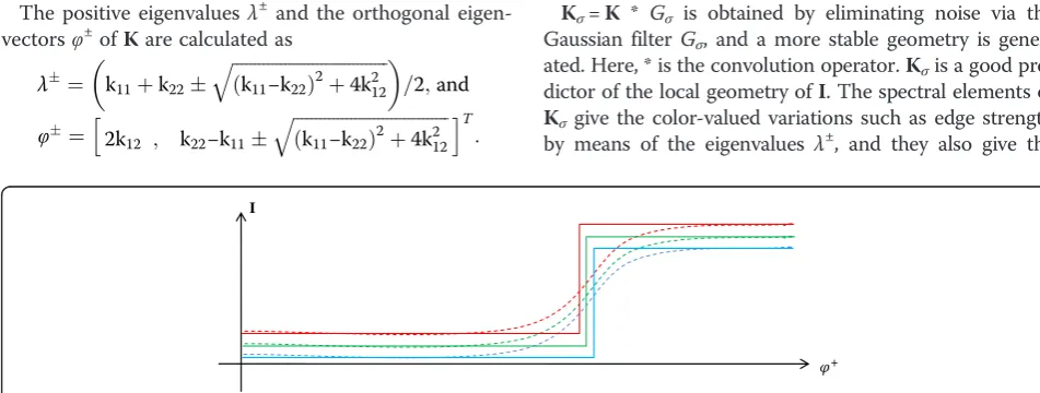
Kσ=K * Gσ is obtained by eliminating noise via the Gaussian filter Gσ, and a more stable geometry is gener-ated. Here, * is the convolution operator.Kσis a good pre-dictor of the local geometry ofI. The spectral elements of Kσgive the color-valued variations such as edge strength by means of the eigenvalues λ±, and they also give the
I
Figure 6Vector edge enhancement (solid lines) based on vector shock filter.Each image channel smoothed (dashed lines) is sharpened without blurring artifact.
Image contour
(a)
(b)
(c)
(d)
(e)
(f)
Figure 5Color image with vector geometries.Graphical representation of two orthogonal eigenvectors on a current pointp (a). Some two orthogonal eigenvectors depicted(b), vector edge indicator function g = (1 +λ+λ−)−1(c), vector gradient norm calculated bypffiffiffiffiffiλþ(d), vector
gradient norm calculated bypffiffiffiffiffiffiffiffiffiffiffiffiλþ−λ−(e), and vector gradient norm calculated byjj∇Ijj ¼pffiffiffiffiffiffiffiffiffiffiffiffiffiffiffiffitraceð ÞK ¼
ffiffiffiffiffiffiffiffiffiffiffiffiffiffiffiffiffiffiffiffiffiffiffi
X3
i¼1jj∇Iij q
corners and edge directions of the local image structures by means of the eigenvectors φ− ⊥ φ+ (Figure 5). More clearly, eigenvalues λ± give some information about the active point as follows:
1. Ifλ+≅λ−≅0, then the point may be in a homogenous region.
2. Ifλ+≫λ−, then the point may be on an edge.
3. Ifλ+≅λ−≫0, then the point may be on a corner.
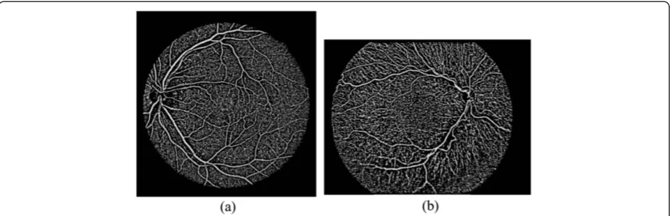
Tschumperlé et al. [39] suggested designing a particu-lar field T: Ω→P(2) of diffusion tensors to define the specification of the local smoothing method for the regularization process. It should be noticed that T, Figure 7Image features of the green channel components for retinal fundus images in Figure 1.Edges from phase map [24](a, b). Note that extremely slim vessel could not be smoothly estimated.
depended on the local geometry ofI, can be defined in terms of the spectral elementsλ±andφ±ofKσ.
T¼s−λþ;λ− φ−φ−Tþsþλþ;λ− φþφþT:
Here, s±: ℝ2→ ℝ are smoothing functions (along φ±), and they change depending on the type of application. Sample functions for image smoothing are proposed in [39] ass−λþ;λ− ¼1þλþþλ− −a1
andsþλþ;λ− ¼
(a)
(b)
(c)
(e)
(f)
(g)
(i)
(j)
(k)
(d)
(h)
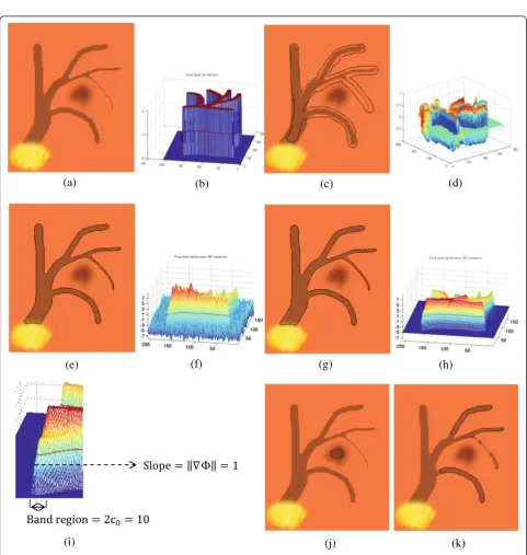
Figure 9Level set evolution.Synthetic image(a), initialization of the level set function with a binary function using c0= 5(b), and its initial
zero-level contour(c), image edges from modified phase map(d), final level set contours based on the proposed method using the potential functionP1
(e), and its level set function(f), final level set contours based on the proposed method using the potential functionP2(g), and its level set function
after 451 iterations(h), slope of final level set function in a band region with size of 2c0(i), final zero-level contours of the given image based on DRLSE
[25] using the potential functionP2and set by a negative-valuedα(j)and a positive-valuedα(k). In(g), with area functionalA(.), the initial contour is
1þλþþλ− −a2;
where a1<a2. The goals of smooth-ing operation are
1. To process pixels on image edges along theφ− direction (anisotropic smoothing)
2. To process pixels on homogeneous regions on all possible directions (isotropic smoothing). In this case,T≅identity matrix and then the method behaves as a heat equation
The regularization approach presented by Tschumperlé et al. [39] is used to obtain the local smoothing geometry T, based on the trace operator:
∂I=∂t¼∂Ii=∂t¼traceðTHiÞ ð2Þ
where Hi is the Hessian matrix of Ii: Hi¼ ∂2I
i=∂x2 ∂2Ii=∂x∂y ∂2I
i=∂y∂x ∂2Ii=∂y2
:
To sharpen the color images, the shock filter is applied on each image channelIionly in one directionφ+ of the vector discontinuities [39]. Moreover, a weighting function is added to enhance color image structure without chan-ging the flat regions. As depicted in Figure 6, such a filter is formulized as follows [39]:
∂Ii=∂t¼ sþ λþ;λ−
−1
sign φþTHiφþ
Iið Þφþ
; where
Iið Þφþ ¼φ−E−þφþEþ;
E−¼
(
0 if ∂Ii bð Þ
∂x
∂Ii fð Þ
∂x <0 min ∂Ii bð Þ
∂x ; ∂Ii fð Þ
∂x
else
Eþ¼
0 if ∂Ii bð Þ
∂y
∂Ii fð Þ
∂y <0 min ∂Ii bð Þ
∂y ; ∂Ii fð Þ
∂y else 8 > > < > > :
ð3Þ
Here,s+:ℝ2→ ℝ, s+(.) = (1 +λ++λ−)−0.5is a decreasing function, and sub-indexes b and f stand for backward and forward finite differences, respectively.
The methods based on color information are com-patible with all local geometric properties expressed above: I(t + 1)=I(t)+τ1∂I(t)/∂t, where τ1 is an adapting
time step. The adapting time step τ1 is set by the
fol-lowing inequality: τ1≤20/max(maxp(∂I(t)(p)/∂t), minp
(∂I(t)(p)/∂t)).
3.2 Modified phase map estimation
Another important step followed in preprocessing retinal fundus images is developing an efficient method for esti-mation of the image structures in cases, for instance, where retinal vessel network contains slim and lengthy vessels with weak edge intensities. According to our ex-periment, edge-based level set image segmentation methods give the best results on images that have only structure information in the segmented regions. Al-though the method [25] described above could segment objects in MRIs and other common medical image for-mats with reasonable success, it may fail to segment ret-inal vasculature successfully, due to vessels with weak edge properties. Therefore, an alternative image struc-ture based on the phase map of the image is employed. It should be noted that neither the phase congruency-based method [40] nor the phase map-congruency-based approach [24] (see Figure 7) generates adequate structure informa-tion for segmentainforma-tion of vasculature in fundus images [30]. Therefore, we combine these two methods as de-scribed below to improve the phase map.
The log-Gabor filter can efficiently extract image fea-tures such as edges and corners without missing any weak object boundaries. This filter, generated in frequency do-main, is a version of logarithmic transformation of the
Gabor filter [4], and it has no DC component. In polar co-ordinates, the filter consists of two components, the radial part and the angular part. These two components are combined to create the log-Gabor filter, which is the transfer function formulated as follows [40]:
Glðr;θÞ ¼ exp −
logðr=f0Þ
ð Þ2
2σr2 −
θ−θ0
ð Þ2
2σθ2 !
:
Here, (r, θ) stands for the polar coordinates, f0 is the
center frequency, θ0is the orientation angle (direction),
σr= log(υ/f0) defines the scale bandwidth, andσθdefines the angular bandwidth. In order to keep the shape ratio of the filter constant, the term υ/f0 must also be kept
constant for varyingf0[40].
The log-Gabor filter can be efficiently used to generate the phase map instead of the gradient norm in image segmentation [24,40]. The image is filtered at different scales in at least three uniformly distributed directions to grab the poor contrast and vasculature with varying width [24]. The filter output is complex in the time do-main, where real and imaginary parts consist of line and edge information, respectively. Filter responses in each scale for all directions must be combined to obtain a ro-tationally invariant phase map. The absolute value of the imaginary parts is taken to avoid an elimination [24].
With these in mind, the modified phase map q is ob-tained as in Equation 4:
q¼
XO
k¼1
XS
l¼1jjqk;ljj
βq
k;l
XO
k¼1
XS
l¼1jjqk;ljj
β : ð4Þ
Here, qk;l¼ℜ qk;l
þ ℑ qk;l
pffiffiffiffiffiffi−1,Ois the number of the orientation angles,Sis the number of the scales,qk;l
is the filter response based on the corrected phase, andβ is a weighting parameter. The normalization q^¼ qjjqjj=
jjq2þσq2
is also used to regularize the phase map. Here, σqstands for a threshold used to reduce noise effect [24]. Since edges align with the zero crossings of the real part of the phase map, the functionℜð Þq^ can be used to estimate image edges as in [24]. Moreover, ℑð Þq^ gives image lines, and the norm of the filter response, formulated asffiffiffiffiffiffiffiffiffiffiffiffiffiffiffiffiffiffiffiffiffiffiffiffiffiffiffiffiffiffiffi jjq^jj ¼
ℜð Þ^q 2þℑð Þq^ 2 q
, gives the strength of the image struc-ture. So, the image structures of the green channel of ret-inal fundus images are estimated efficiently and correctly by using the log-Gabor filter as seen in Figure 8.
3.3 Structure-based level set segmentation method A novel structure-based variational method is proposed in this study in order to trace retinal vasculature. The level set function in [25] can be discretized more easily compared to
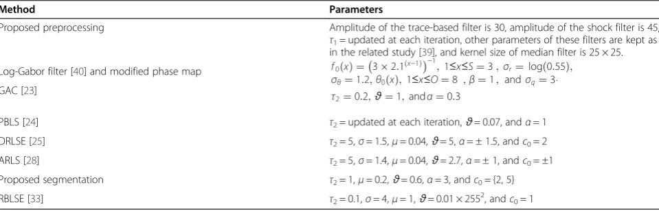
Table 2 Parameter values of the methods
Method Parameters
Proposed preprocessing Amplitude of the trace-based filter is 30, amplitude of the shock filter is 45,
τ1= updated at each iteration, other parameters of these filters are kept as
in the related study [39], and kernel size of median filter is 25 × 25.
Log-Gabor filter [40] and modified phase map f0ð Þ ¼x 32:1ðx−1Þ
−1
;1≤x≤S¼3;σr¼log 0ð:55Þ;
σθ¼1:2;θ0ð Þx;1≤x≤O¼8 ;β¼1; andσq¼3⋅
GAC [23]
τ2¼0:2;ϑ¼1;andα¼0:3
PBLS [24] τ2= updated at each iteration,ϑ= 0.07, andα= 1
DRLSE [25] τ2= 5,σ= 1.5,μ= 0.04,ϑ= 5,α= ± 1.5, andc0= 2
ARLS [28] τ2= 5,σ= 1.4,μ= 0.04,ϑ= 2.7,α= ± 1, andc0= ±1
Proposed segmentation τ2= 1,μ= 0.2,ϑ= 0.6,α= 3, andc0= {2, 5}
RBLSE [33] τ2= 0.1,σ= 4,μ= 1,ϑ= 0.01 × 255
2
, andc0= 1
Table 1 Formulas of some variational image segmentation methods
Group Method Formula
Edge-based GAC [23] ϑk k∇Φ div g k k∇∇ΦΦþ αgk k∇Φ
PBLS [24] ϑjj∇Φjjdivjj j∇∇ΦΦj−αjj∇Φjjℜð^qPBLSÞ
DRLSE [25] μdivðDðjj j∇ΦjÞ∇ΦÞ þϑδεð ÞΦdiv g jj j∇∇ΦΦjþ αgδεð ÞΦ
ARLS [28] μ ∇2Φ−div ∇Φ
∇Φ
k k
þϑδεð ÞΦdivk k∇Φ sð∇ðIGσÞÞ−2∇Φþ αδ
εð ÞΦ∇2ðIGσÞ
Region-based RBLSE [33] μdivðDðjj j∇ΦjÞ∇ΦÞ þϑδεð ÞΦdivjj j∇∇ΦΦj−αδεð ÞΦðe1−e2Þ;
other methods in the literature since it has a level set regularization term. The discretization process uses cen-ter/forward difference model instead of other complex discretization schemes [23,24]. For instance, in the GAC model in [23], the upwind method is used for the calcula-tion of the gradient norm of the level set funccalcula-tionΦ, and for the re-initialization of the level set function Φ, essen-tially non-oscillatory (ENO) scheme is employed. There-fore, the same level set function regularization term of the DRLSE method [25] is used in the proposed method.
In the DRLSE method [25], the formulas of R(Φ) =∫Ω
P(Φ)dp, L(Φ) =∫Ω gδε(Φ)||∇Φ||dp and A(Φ) =∫Ω
gHε(−Φ)dp are employed for segmentation. Here, P(.) is a potential function. The length functionalL(.) smoothes the zero-level contour. The area functionalA(.) helps ac-celerate the level set evolution when the initial contour is located far away from the object boundaries. For dem-onstration, see Figure 9.
In edge-based level set approaches, a smooth edge indicator function is generally obtained from the gra-dient norm of the Gaussian-filtered image. One choice isg= (1 + ||∇(Gσ *I)||2)−1. The edge indicator function
g carries key information to locate the zero-level con-tour. Hεandδε¼H0ε are finite-width approximations
of the Heaviside function and Dirac-delta forε:
Hεð Þ ¼x
(
12 1þ
π εþ
1
πsin πx
ε
;j jx≤ε
1; x>ε
0; x<−ε
and
δεð Þ ¼x 1
2ε 1þ cos
πx
ε
h i
;j jx≤ε
0; j jx >ε
(
where, in general, the parameterεis set to 1.5.
The level set function regularization term should have a minimum to maintain the signed distance property of ||∇Φ|| = 1 in a band region around the zero-level contour as depicted in Figure 9i, instead of the heat equation [25] that enforces ||∇Φ|| = 0, even-tually. So, the solution, based on the potential function
P1(||∇Φ||) = 0.5(||∇Φ||−1)2, is formulated as follows
[25]:
(a)
(b)
(c)
(d)
(e)
(f)
∂ΦR
∂t ¼μdivðDðjj∇ΦjjÞ∇ΦÞ ¼μ ∇
2Φ−div ∇Φ
∇Φ
j j j j
ð5Þ
The sign ofD(||∇Φ||) = 1−(1/||∇Φ||), whereD(x) =x−1
∂P(x)/∂x indicates the property of the diffusion term
based on anisotropic regularization in the following two cases [25]:
1. For ||∇Φ|| > 1, the diffusion rateμD(.) is positive and the diffusion is forward, which decreases the term ||∇Φ||
2. For ||∇Φ|| < 1, the diffusion is backward, which increases the term ||∇Φ||
However, this regularization term may cause an unsatis-factory result on the level set function when ||∇Φ|| is close to 0 outside the band region as shown in Figure 9e,f. So, as given in Figure 9g,h, a corrected potential function is given as follows [25]:
P2ð Þ ¼x
1 2π
ð Þ2ð1−cos 2ð πxÞÞifx≤1
1 2ðx−1Þ
2
ifx≥1⋅ 8
> < > :
In the proposed method, the initial contours have to be set automatically around vessels in order to find the global minimum in a segmented image correctly. Sometimes, there is a risk of getting stuck in a local minimum due to the fact that retinal fundus images include defects such as drusen, GA, etc. So, seed points should be chosen around vessel regions to gen-erate a desirable result. Note that the seed points can be set in or out of vessel areas, but they should be very close to the vessel structures (compare Figures 9 and 10). There is another approach, called the ARLS method [28] in the literature, utilizing automatic initial contours based on Laplacian of Gaussian (LoG) filter. This method is not proper for segmenting retinal vas-culature, as the filter is very sensitive to noise, and there is a risk in the automatic initial contours if the retinal fundus image contains pathological regions. On the contrary, in the proposed method, the real part of the modified phase map has zero-crossing boundaries, and the method ensures to find the global minimum if the initial contour is selected around vasculature
regions (Figure 9a,b,c,d,e,f,g,h). Therefore, we improve the speed term based on the area functional A(.) as follows:
∂ΦA
∂t ¼−αδεð ÞℜΦ ð Þq^ ⋅ ð6Þ
In our method, iso-contours automatically shrink when the contour is outside the object due to the func-tional of A(.) returning a positive contribution, or they automatically expand with a negative value inA(.) when the contour is inside, regardless of the sign of α values as in the existing method [25] (Figure 9j,k).
To eliminate staircasing effect [41] and not to miss weak object boundaries [28], a potential function based on weighted total variation (WTV) model is used asP3ð Þ ¼Φ
∇sð∇ðIGσÞÞ
sð∇ðIGσÞÞ. Here,s:ℝ →[1,2) is a monotonically decreasing function [27,28,41]. Such a function used in the ARSL method [28] is not capable of regularizing zero-level con-tours because of the smoothed gradient norm which can-not generate image structure. Furthermore, the total variation (TV) model, presented in the PBLS method [24], will not smooth zero-level contours completely, generat-ing unsatisfactory results. Therefore, we suggest a modi-fied oriented Laplacian flow as in Equation 7, originally employed in image denoising [39,42], in order to regularize the zero-level contour:
∂ΦL
∂t ¼ϑδεð ÞΦ Φξξþsðk kq^ ÞΦηη
ð7Þ
where sðj jj jq^ Þ ¼1þ jj^qjj2 −1, Φζζ=ζTHζ, Φηη=ηTHη, and His the Hessian ofΦ. The unit vectorsηand ζare represented by the gradient direction and the tangential
(a)
(b)
(c)
Figure 13Level set evolution with setting parameter values for a non-pathological image obtained from DRIVE dataset.ϑ= 0.4 and
(its orthogonal) direction, respectively. Here, η=∇Φ/ ||∇Φ|| and ζ=η⊥. s(.) depends on the value of the strength of the image structure jj^qjj, which is generated from phase map. So, along the zero-level contour, the oriented Laplacian flow has a strong smoothing effect. As a result, our approach is more efficient compared to the PBLS method [24] to regularize zero-level contours.
3.4 Proposed segmentation method
The proposed method accepts a retinal fundus image in
RGB color space as input. Firstly, a simple mask is ob-tained to exclude the exterior parts of the fundus where the color is in the 0-U interval in all three channels (generally very dark regions). Also, an iterated erosion op-erator whose structure element isB¼½0; 1; 0; 1;1; 1;
(a)
(b)
(c)
(d)
(e)
(f)
(g)
(h)
(i)
0; 1; 0T is applied on the mask for proper execution. Secondly, a preprocessing step is employed to obtain a corrected image in terms of intensity inhomogeneity. Thirdly, we compute the phase map by using the cor-rected image as input. Afterwards, to eliminate some small non-blood vessels region, Otsu’s method [43] is applied on the processed image. As a result of these processes, a skeleton-based image giving the centerlines of the vascula-ture is generated with the following steps: (i) remove dis-connected pixels, (ii) obtain skeleton-based image, (iii) find junctions, (iv) trace lines (centerlines) and label them, and (v) clean short lines. Here, a threshold value is used to eliminate tiny little short lines called artifacts.
In order to set the optimum initialization of the zero-level contour, seed points have to be selected around the vasculature according to the centerline obtained based on phase map properties. Here, a morphological dilation op-erator whose structure element isB¼½1; 1; 1; 1;1; 1; 1; 1; 1T, is performed on the centerlines to generate a proper initial contour. Finally, the proposed method cre-ates the output by using the structure-based level set method. Our level set function is minimized by using Euler Lagrange and the iterative gradient descent proced-ure as follows:
∂Φ
∂t ¼μdivðDðjj∇ΦjjÞ∇ΦÞ þϑδεð ÞΦ
Φζζþsðj jj jq^ ÞΦηη −αδεð ÞΦℜð Þq^ ⋅ ð8Þ
Note that values of the edge indicator functiong, used in [25], are in the [0,1] interval. In the proposed method, the sign of the coefficient αin the level set energy func-tional can always remain positive in contrast to the earlier method [25] since the function ℜð Þq^ obtained from the phase map has a different sign around object boundaries.
The proposed level set evolution equation culminates in
Φ(t+ 1)=Φ(t)+τ2∂Φ(t)/∂twhereτ2is a time step, which is
set by τ2≤(4μ)−1 based on Courant-Friedrichs-Lewy
(CFL) condition with 4-neighbor connectivity [25,44]. The initialization of level set function is important. If the seed points are selected away from the vessel centers and close to pathological regions, the proposed method can fail (wrongly segmenting the pathological region, as well) as shown in Figure 10d.
4 Experimental results
The proposed method is tested on DRIVE [3], STARE [11], and our own datasets [2,19] for this study. Our 34 wide-angle fundus images are grabbed from premature infants supplied by the RetCam II camera and delineated by medical experts. The images from different experts are combined to create one ground truth image for each one of the fundus image [1,2]. Some methods used in this study are summarized in Table 1. The chosen pa-rameters of the algorithm are given in Table 2. Eight uniformly distributed angle directions and three image re-sampling scales for the log-Gabor filter are used in the method. The maximum number of iterations for the
main algorithm depends on the radii of the vessel, and for this study, it is experimentally set as 60 + 1 (extra regularization of the zero-level contour via level set evo-lution withα= 0). The threshold values ofUfor creating mask images are set to 40, 40, and 45, for DRIVE data-set, our datadata-set, and STARE datadata-set, respectively. More-over, small gaps in the created mask image for STARE dataset are filled using a morphological closing operator whose structure element is a disk of radius 10. In order to eliminate the out of fundus image region, the num-bers of iterated erosion operator are set to 8, 8, and 2 for DRIVE dataset, our dataset, and STARE dataset, re-spectively. The threshold values of short line length are set as 15, 35, and 15 for DRIVE dataset, our dataset, and STARE dataset, respectively. c0values for initializing of
level set functions are set to 5, 5, and 2 for DRIVE
dataset, our dataset, and STARE dataset, respectively. Here, in all cases except for the 20th image from STARE dataset, second selection is used for preprocessing. First selection is used for preprocessing on 20th image from STARE dataset because this image does not have inten-sity inhomogeneity. The Neumann boundary condition is employed [25] to solve Equation 8.
The results of the preprocessing step for some test im-ages from DRIVE dataset are seen in Figures 11 and 12. Using the segmented image, on which a scalar approach [19,38] is applied for the preprocessing step, the vascula-ture cannot be traced truly. This does not happen in our method because we use a trace-based method to smoothen and then a shock filter to sharpen the given image. Both filters work based on the color information unlike the ones in the scalar approach presented in
[19,38]. Therefore, the image, obtained by our method, is denoised more efficiently and segmented more cor-rectly. While our method produces promising results, we should also indicate that there are still missed retinal vessels. Those missed vessels are very thin with weak edge properties. There are regular retinal vessels with normal dimensions wholly missed with the preprocess-ing step presented in [19]. Such a region is marked with a blue circle as shown in Figure 11f. In Figure 12b, a dif-ference image between input color image and smoothed version of the input image is shown. The blue channel
has noise and seems to contain higher frequencies com-pared to Figure 11b. Furthermore, images that could not be segmented using the proposed structure-based level set segmentation method without preprocessing are shown in Figure 12g,h.
Figure 13 demonstrates the results of the level set function evolution based on setting the coefficient values ϑ and α used in the length term regularizing zero-level contour and the speed term accelerating the level set function evolution.ϑis set to 0.4, 0.8, and 1, andαis set to 1.5, 2.5, and 3, respectively, as shown Figure 13a,b,c.
However, some retinal vessels (marked with a blue cir-cle) are still not connected. Therefore, in order to gener-ate a good result as seen in Figure 12f,ϑandαare set to 0.6 and 3, respectively.
Our segmentation process illustrated in Figure 14 em-ploys the skeletonized version of the input image on
which a morphological dilation operator is performed only once to initialize the level set function. The pro-posed method generates good results; some very thin retinal vessels with poor contrast are still missed due to the fact that our method is unable to produce a proper phase map. However, unlike previous works [24,25], the
(a)
(b)
(c)
(d)
(e)
(f)
(g)
(h)
(i)
method can trace retinal vessels efficiently, since the structure-based level set segmentation method is able to shrink or expand automatically as displayed in Figure 14h where the level set function is initialized inside the vessels in some regions and outside the vessels in some regions.
The test results of preprocessing operations on our dataset are shown Figure 15. The non-uniform intensities in the given image are estimated and corrected properly.
A sample vessel segmentation result for a non-pathological fundus image from our dataset is shown in Figure 16. Here, the approach cannot trace some vessels with poor contrasts as seen in Figure 16h. Also, the image could not be segmented employing the proposed segmentation method without preprocessing as depicted in Figure 16g.
Another sample vessel segmentation result for a non-pathological fundus image from STARE dataset is depicted in Figure 17. Here, the vessels can be traced properly using the method.
The results of other test images in DRIVE, our im-ages, and STARE datasets are given in Figures 18, 19 and 20. Some segmentation results for pathological im-ages include artifact, and they are marked with blue cir-cles. These regions have also poor contrast, and retinal vessels in these regions are very thin.
Figure 21 depicts another case, for which both methods described in earlier work [24,25] failed espe-cially at regions with poor contrast. However, the pro-posed method is able to properly track the vessels in those regions as shown in Figure 21e. Although the
(a)
(b)
(c)
(d)
(e)
(f)
PBLS method presented in [24] runs faster than ours since it employs a narrow band implementation, that faster method is unable to trace retinal vessels properly due to the fact that the phase map of the method is not estimated correctly in the regions with thin vessels and poor contrasts. Also, the DRLSE method proposed in [25] does not expand the vessels if the initialization starts inside the vessel. On the other hand, if initialization starts outside the vessel and the image is in
poor contrast, the DRLSE method over-segments the vessels because it uses the image gradient instead of the phase map. Instead of a TV approach, ∂ΦL=∂t¼ϑδεð ÞΦ
div gjj∇Φ∇Φjj
; if an oriented Laplacian flow approach, ∂ΦL/∂t=ϑδε(Φ)(Φζζ+gΦηη), proposed in our work, is employed in the DRLSE method to smooth zero-level contours, the results may visually seem to be like over-smoothing as displayed in Figure 21b,c. But, as depicted
(a)
(b)
(c)
(d)
(e)
(f)
in Figure 21e, this disadvantage turns into an advantage if the modified oriented Laplacian flow approach,∂ΦL=∂
t¼ϑδεð ÞΦ Φηηþsðj jj jq^ Þ ΦηηÞ , is employed in our method, since it eliminates the expansion of segmented vessel areas. As shown in Figure 21d, the expansion is not completely eliminated if a modified TV approach, ∂ ΦL=∂t¼ϑδεð ÞΦ divðsðj jj jq^ Þ∇Φ=jj∇ΦjjÞ, is used in our
method. Also, the vessels could be traced more properly in the proposed method, if the iteration number is in-creased, but this increases the cost. The result of our method seems to be more efficient compared to the existing methods [24,25] in the literature since it has a novel zero-level contour regularization term and it em-ploys a modified phase map.
Lastly, the segmentation results of the non-pathological image generated by the region-based level set evolution
method (RBLSE) [33] are given in Figure 22. The most im-portant advantage of this method is that the initialization may start on any region of the fundus image instead of around vessels by a simple selection. The segmentation of vessels can be done in the fundus images without poor contrast in the initialization phase. After that, while some segmented vessels are combined, some gradually disap-peared in later iterations. But surprisingly, after the 42nd iteration, all segmented vessels are gone and only the boundary of the retina remains as segmented as presented in Figure 22c.
Quantitative results are obtained for both datasets where manual vessel segmentation labeling was per-formed and verified by medical experts. Comparing the results with manual delineations, we obtain overall stat-istical quality metrics such as sensitivity Se, specificity
(d)
(e)
(a)
(b)
(c)
Sp, positive predictive value Ppv, negative predictive value Npv, accuracy Acc [14], and kappa κ [45]. These measures are given as follows:
Se¼ TP
TPþFN; Sp¼
TN
TNþFP ; Ppv¼
TP TPþFP;
Npv¼ TN
TNþFN ; Acc¼
TPþTN
TPþFPþTNþFN;
and κ¼ 2 TPð TN−FPFNÞ TPþFP
ð ÞðFPþTNÞ þðTPþFNÞðFNþTNÞ:
ð9Þ
Here, TP refers to a pixel labeled as vessel by both the algorithm and the medical experts’ ground truth data, while TN refers to a pixel that is deemed to be non-vessel by both. FN refers to pixels of non-vessels (according to ground truth data) missed by the algorithm, and FP refers to pixels falsely categorized by the algorithm as vessel. In order to compare the proposed method, the same statistical metrics for supervised and unsupervised methods [11,14-17] on DRIVE dataset, our dataset, and STARE dataset are also reported in Tables 3, 4, 5, and 6. Here, it should be addressed that, although vascular seg-mentation has been achieved in countless studies, some of which even have better results in the literature, it has not been done so far using structure-based level set ap-proach. In addition, for instance, while the unsupervised method [17] has good accuracy metric results, it gener-ates occasional artifacts, such as false vessels, next to the optic disks. The results of our method are promising due to the fact that the method does not use any train-ing algorithm compared to the supervised methods pre-sented in [14-17]. As can be seen in Table 6 from the
Acc and κ metrics, for instance, when compared with PBLS method, our method fairs better quantitatively.
The methods are implemented using MATLAB R2010a. The programs are executed on a laptop with a Pentium 2.20-GHz processor and a 2-GB RAM. The segmentation of the retinal fundus image with a size of 565 × 584 pixels, as depicted in Figure 12f, lasts 61 iterations and 92.69 s. Note that the run time of the program may vary according to structure and size of the retinal fundus image.
5 Conclusions
We present a structure-based level set method with automatic seed point selection for segmentation of ret-inal vasculature in fundus images. Extensive experiments employing the proposed algorithms using datasets indi-cate that the algorithm performs well and favorably compared to the already existing level set-based methods in the literature. Developing strategies to improve incon-sistencies in clinical diagnosis is an important challenge in ophthalmology. The segmentation methods described in this study may provide a basis for the development of computer-based image analysis algorithms. Future work will involve quantitative feature extraction from seg-mented retinal vessels, followed by implementation of these image analysis algorithms for image-based diag-nostic assistance.
We plan to extend the study in order to improve the results especially for pathological regions such as drusen, GA, etc. Moreover, we will investigate how to use all color channels of the given image interactively in an effi-cient manner in order to trace retinal vasculature more properly. In addition to this, we plan to do a narrow band implementation in order to accelerate the run time of the proposed method.
Table 4 Statistical results of our method for test images of 1 to 20 from our dataset
Dataset Image number Se Sp Ppv Npv Acc κ
Ours 1 0.4821 0.9905 0.7483 0.9702 0.9623 0.5676
2 0.3471 0.9887 0.6680 0.9586 0.9494 0.4330
3 0.5745 0.9786 0.5802 0.9781 0.9589 0.5557
4 0.5617 0.9695 0.5911 0.9657 0.9398 0.5437
5 0.5699 0.9872 0.7537 0.9708 0.9602 0.6284
6 0.3527 0.9879 0.6416 0.9613 0.9511 0.4318
7 0.8109 0.9566 0.5234 0.9885 0.9485 0.6098
8 0.3134 0.9887 0.6280 0.9594 0.9499 0.3950
9 0.3966 0.9857 0.5666 0.9719 0.9591 0.4461
10 0.4290 0.9878 0.5958 0.9764 0.9654 0.4814
11 0.2789 0.9901 0.6119 0.9607 0.9523 0.3619
12 0.5497 0.9840 0.6101 0.9796 0.9651 0.5602
13 0.6942 0.9783 0.6056 0.9852 0.9653 0.6288
14 0.4028 0.9844 0.5128 0.9759 0.9616 0.4316
15 0.5848 0.9849 0.5977 0.9840 0.9700 0.5756
16 0.3300 0.9877 0.6573 0.9539 0.9440 0.4133
17 0.7426 0.9731 0.5785 0.9870 0.9622 0.6308
18 0.5550 0.9762 0.5149 0.9797 0.9578 0.5122
19 0.7238 0.9712 0.6101 0.9826 0.9567 0.6392
20 0.6576 0.9680 0.4891 0.9838 0.9542 0.5373
Table 3 Statistical results of our method for test images of 1 to 20 from DRIVE dataset
Dataset Image number Se Sp Ppv Npv Acc κ
DRIVE 1 0.8182 0.9581 0.7461 0.9723 0.9398 0.7457
2 0.7764 0.9654 0.7982 0.9608 0.9371 0.7502
3 0.7387 0.9513 0.7218 0.9551 0.9202 0.6834
4 0.7456 0.9677 0.7826 0.9607 0.9378 0.7279
5 0.7419 0.9682 0.7878 0.9593 0.9371 0.7279
6 0.7142 0.9726 0.8126 0.9534 0.9358 0.7233
7 0.7507 0.9466 0.6846 0.9609 0.9204 0.6699
8 0.7285 0.9619 0.7332 0.9610 0.9325 0.6923
9 0.7223 0.9738 0.7880 0.9630 0.9439 0.7221
10 0.7535 0.9656 0.7507 0.9661 0.9400 0.7179
11 0.7456 0.9512 0.6972 0.9613 0.9243 0.6768
12 0.7932 0.9594 0.7391 0.9697 0.9383 0.7297
13 0.7165 0.9665 0.7811 0.9533 0.9307 0.7073
14 0.7940 0.9573 0.7130 0.9720 0.9380 0.7160
15 0.7867 0.9463 0.6321 0.9742 0.9296 0.6616
16 0.7880 0.9697 0.7989 0.9677 0.9457 0.7621
17 0.7581 0.9715 0.7900 0.9660 0.9451 0.7425
18 0.8407 0.9517 0.6965 0.9784 0.9388 0.7271
19 0.8696 0.9599 0.7504 0.9815 0.9489 0.7764
Table 6 Statistical average results for test images of 1 to 20 from the datasets
Dataset Method Se Sp Ppv Npv Acc κ
DRIVE Unsupervised PBLS [24] 0.7754 0.9348 0.6403 0.9655 0.9140 0.6494
Jiang et al. [12] - - - - 0.9212
-Martinez-Perez et al. [13] 0.7246 0.9655 - - 0.9344
-Proposed 0.7704 0.9613 0.7460 0.9658 0.9365 0.7198
Budai et al. [17] 0.6440 0.9870 - - 0.9572
-Supervised Staal et al. [16] 0.7194 0.9773 - - 0.9442
-Marin et al. [14] 0.7067 0.9801 0.8433 0.9582 0.9452
-Soares et al. [15] 0.7283 0.9788 - - 0.9466
-Ours Unsupervised PBLS [24] 0.6600 0.9482 0.4380 0.9804 0.9328 0.4754
Proposed 0.5179 0.9810 0.6042 0.9737 0.9567 0.5192
STARE Unsupervised PBLS [24] 0.8268 0.9117 0.5227 0.9803 0.9035 0.5822
Hoover et al. [11] 0.6751 0.9567 - - 0.9267
-Martinez-Perez et al. [13] 0.7506 0.9569 - - 0.9410
-Proposed 0.6926 0.9726 0.7633 0.9656 0.9441 0.6779
Supervised Soares et al. [15] 0.7103 0.9737 - - 0.9480
-Staal et al. [16] 0.6970 0.9810 - - 0.9516
-Marin et al. [14] 0.6944 0.9819 - - 0.9526
-Table 5 Statistical results of our method for test images of 1 to 20 from STARE dataset
Dataset Image number Se Sp Ppv Npv Acc κ
STARE 1 0.6449 0.9731 0.7455 0.9574 0.9374 0.6570
2 0.5754 0.9836 0.7795 0.9584 0.9464 0.6336
3 0.8036 0.9519 0.5973 0.9820 0.9398 0.6527
4 0.3117 0.9972 0.9275 0.9271 0.9271 0.4376
5 0.8084 0.9466 0.6803 0.9723 0.9296 0.6985
6 0.7759 0.9666 0.6912 0.9781 0.9498 0.7035
7 0.8567 0.9631 0.7412 0.9820 0.9514 0.7674
8 0.7758 0.9644 0.7125 0.9742 0.9451 0.7121
9 0.7814 0.9698 0.7569 0.9736 0.9495 0.7406
10 0.7568 0.9722 0.7711 0.9700 0.9485 0.7349
11 0.8000 0.9629 0.7004 0.9780 0.9470 0.7175
12 0.8446 0.9665 0.7490 0.9814 0.9537 0.7679
13 0.7743 0.9710 0.7881 0.9687 0.9470 0.7510
14 0.7611 0.9739 0.8055 0.9663 0.9474 0.7528
15 0.6239 0.9796 0.8031 0.9512 0.9376 0.6680
16 0.4445 0.9916 0.8961 0.9165 0.9150 0.5528
17 0.7238 0.9803 0.8372 0.9621 0.9488 0.7477
18 0.5669 0.9931 0.8594 0.9685 0.9635 0.6647
19 0.4183 0.9934 0.8001 0.9646 0.9595 0.5304
Competing interests
The authors declare that they have no competing interests.
Acknowledgements
This work is partially supported by grants from TUBITAK (grant no. 1059B191000548), NSF, and NIH.
Author details
1Department of Computer Engineering, Karadeniz Technical University,
Trabzon 61080, Turkey.2Cognitive Systems Laboratory, Northeastern
University, Boston, MA 02115, USA.3Martinos Imaging Center, Massachusetts
General Hospital, Boston, MA 02129, USA.4Department of Ophthalmology,
Oregon Health & Science University, Portland, OR 97239-3098, USA.
5Department of Medical Informatics, Oregon Health & Science University,
Portland, OR 97239-3098, USA.
Received: 27 February 2014 Accepted: 30 July 2014 Published: 11 August 2014
References
1. MF Chiang, L Jiang, R Gelman, YE Du, JT Flynn, Interexpert agreement of plus disease diagnosis in retinopathy of prematurity. Arch. Ophthalmol 125, 875–880 (2007)
2. R Gelman, L Jiang, YE Du, ME Martinez-Perez, JT Flynn, MF Chiang, Plus disease in retinopathy of prematurity: pilot study of computer-based and expert diagnosis. JAAPOS11(6), 532–540 (2007)
3. A Osareh, B Shadgar, An automated tracking approach for extraction of retinal vasculature in fundus images. J. Opthalmic. Vis. Res. 5, 20–26 (2010)
4. D Wu, M Zhang, JC Liu, W Bauman, On the adaptive detection of blood vessels in retinal images. IEEE Trans. Biomed. Eng.53, 341–343 (2006) 5. MZC Azemin, DK Kumar, TY Wong, R Kawasaki, P Mitchell, JJ Wang, Robust
methodology for fractal analysis of the retinal vasculature. IEEE Trans. Med. Imaging2(30), 243–250 (2011)
6. V Mahadevan, H Narasimha-Iyer, B Roysam, HL Tanenbaum, Robust model-based vasculature detection in noisy biomedical images. IEEE Trans. Inf. Technol. Biomed.8(3), 360–376 (2004)
7. H Narasimha-Iyer, V Mahadevan, JM Beach, B Roysam, Improved detection of the central reflex in retinal vessels using a generalized dual-Gaussian model and robust hypothesis testing. IEEE Trans. Inf. Technol. Biomed. 3(12), 406–410 (2008)
8. KW Tobin, E Chaum, VP Govindasamy, TP Karnowski, Detection of anatomic structures in human retinal imagery. IEEE Trans. Med. Imaging
26(12), 1729–1739 (2007)
9. M Niemeijer, X Xu, AV Dumitrescu, P Gupta, B van Ginneken, JC Folk, MD Abramoff, Automated measurement of the arteriolar-to-venular width ratio in digital color fundus photographs. IEEE Trans. Med. Imaging
11(30), 1941–1950 (2011)
10. L Wang, A Bhalerao, R Wilson, Analysis of retinal vasculature using a multiresolution Hermite model. IEEE Trans. Med. Imaging 2(26), 137–152 (2007)
11. A Hoover, V Kouznetsova, M Goldbaum, Locating blood vessels in retinal images by piecewise threshold probing of a matched filter response. IEEE Trans. Med. Imaging19(3), 203–210 (2000)
12. X Jiang, D Mojon, Adaptive local thresholding by verification-based multithreshold probing with application to vessel detection in retinal images. IEEE Trans. Pattern. Anal. Mach. Intell.25(1), 131–137 (2003) 13. ME Martinez-Perez, AD Hughes, SA Thom, AA Bharath, KH Parker,
Segmentation of blood vessels from red-free and fluoresce in retinal images. Med. Image Anal.11(1), 47–61 (2007)
14. D Marin, A Aquino, GME Arias, JM Bravo, A New supervised method for blood vessel segmentation in retinal images by using gray-level and moment invariants-based features. IEEE Trans. Med. Imaging 30(1), 146–158 (2011)
15. JVB Soares, JJG Leandro, RM Jr Cesar, HF Jelinek, MJ Cree, Retinal vessel segmentation using the 2-D Gabor wavelet and supervised classification. IEEE Trans. Med. Imaging25(9), 1214–1222 (2006)
16. J Staal, MD Abramoff, M Niemeijer, MA Viergever, B van Ginneken, Ridge-based vessel segmentation in color images of the retina. IEEE Trans. Med. Imaging 23, 501–509 (2004)
17. A Budai, R Bock, A Maier, J Hornegger, G Michelson, Robust vessel segmentation in fundus images. Int. J Biomed. Imaging
2013, (2013)
18. AF Frangi, WJ Niessen, KL Vincken, MA Viergever,Multiscale Vessel Enhancement Filtering (Springer(Germany, Heidelberg, 1998)
19. S You, E Bas, D Erdogmus, J Kalpathy-Cramer, Principal curve based retinal vessel segmentation towards diagnosis of retinal diseases. Proc. Healthcare Inform, Imaging Sys. Biol. (HISB) 331–337 (2011). San Jose, California, USA, (2011)
20. D Erdogmus, U Ozertem, Self-consistent locally defined principal surfaces. Proc. ICASSPVol. 2, II.549–II.552 (2007). Honolulu, Hawaii, USA
21. C Kirbas, F Quek,Vessel Extraction Techniques and Algorithms: a Survey. Proceedings of the Third IEEE Symposium on BioInformatics and BioEngineering (BIBE’03), 238-245 (Bethesda, Maryland, USA, 2003) 22. L Vese, T Chan, A multiphase level set framework for image segmentation
using the Mumford and Shah model. Int. J. Comput. Vis.50(3), 271–293 (2002)
23. V Caselles, R Kimmel, G Sapiro, Geodesic active contours. Int. J. Comput. Vis. 22(1), 61–79 (1997)
24. G Lathen, J Jonasson, M Borga, Blood vessel segmentation using multi-scale quadrature filtering. Pattern Recogn. Lett.31, 762–767 (2010)
25. C Li, C Xu, C Gui, MD Fox, Distance regularized level set evolution and its application to image segmentation. IEEE Trans. Image Process. 19(12), 3243–3254 (2010)
26. KY Pang, L Iznita, A Fadzil, AN Hanung, N Hermawan, SA Vijanth,
Segmentation of Retinal Vasculature in Colour Fundus Images(Conference on Innovation Technologies in Intelligent Systems and Industrial Applications (CITISIA, Malaysia, 2009), pp. 398–401
27. B Zhou, C Mu, Level set evolution for boundary extraction based on a p-Laplace equation. Appl. Math. Mod34(12), 3910–3916 (2010)
28. L Meng, H Chuanjiang, Z Yi, Adaptive regularized level set method for weak boundary object segmentation. Math. Probl. Eng2012(369472), 16 (2012). doi:10.1155/2012/369472
29. A Belaid, D Boukerroui, Y Maingourd, J-F Lerallut, Phase based level set segmentation of ultrasound images. IEEE Trans. Inform. Tech. Biomed 15(1), 138–147 (2011)
30. B Dizdaroğlu, E Ataer-Cansizoglu, J Kalpathy-Cramer, K Keck, MF Chiang, D Erdogmus,Level Sets for Retinal Vasculature Segmentation Using Seeds from Ridges and Edges from Phase Maps. 2012 IEEE International Workshop On Machine Learning For Signal Processing (Santander, Spain, 2012)
31. G Yu, P Lin, P Li, Z Bian, Region-based vessel segmentation using level set framework. Int. J. Control. Autom. Syst.4(5), 660–667 (2006)
32. C Li, C Kao, JC Gore, Z Ding, Minimization of region-scalable fitting energy for image segmentation. EEE Trans. Image Proc.17(10), 1940–1949 (2008)
33. C Li, R Huang, Z Ding, C Gatenby, DN Metaxas, JC Gore, A level set method for image segmentation in the presence of intensity inhomogeneities with application to MRI. IEEE Trans. Image Proc.20(7), 2007–2016 (2011) 34. YQ Zhao, XH Wang, XF Wang, FY Shih, Retinal vessels segmentation
based on level set and region growing. Pattern Recognition. 47(7), 2437–2446 (2014)
35. M Bertalmio, L Vese, G Sapiro, S Osher, Simultaneous structure and texture image inpainting. IEEE Trans. Image Process.12, 882–889 (2003) 36. A Buades, TM Le, J-M Morel, LA Vese, Fast cartoon + texture image filters.
IEEE Trans. Image Process.19(8), 1978–1986 (2010)
37. B Dizdaroğlu, An image completion method using decomposition. EURASIP J. Advanc. Signal Proc2011(831724), 15 (2011). doi:10.1155/2011/831724 38. MJ Black, G Sapiro, DH Marimont, D Heeger, Robust anisotropic diffusion.
IEEE Trans. Image Process.7(3), 421–432 (1998)
39. D Tschumperlé,PDE’s based regularization of multi-valued images and applications, PhD thesis(Université de Nice-Sophia Antipolis, France, 2002) 40. P Kovesi, Phase congruency: a low-level image invariant. Psychological
Research64(2), 136–148 (2000)
41. P Blomgren, TF Chan, CK Wong, Total variation image restoration: numerical methods and extensions. Proc. IEEE Int. Conf Image Proc3, 384–387 (1997)
43. N Otsu, A threshold selection method from gray-level histogram. IEEE Trans. Syst. Man Cybern9(1), 62–66 (1979)
44. R Courant, K Friedrichs, H Lewvy, Über die partiellen Differenzengleichungen der mathematischen Physik. Math. Ann.100(1), 32–74 (1928)
45. J Landis, G Koch, The measurement of observer agreement for categorical data. Biometrics33, 159–174 (1977)
doi:10.1186/1687-5281-2014-39
Cite this article as:Dizdaroğluet al.:Structure-based level set method for automatic retinal vasculature segmentation.EURASIP Journal on Image and Video Processing20142014:39.
Submit your manuscript to a
journal and benefi t from:
7 Convenient online submission
7 Rigorous peer review
7 Immediate publication on acceptance
7 Open access: articles freely available online
7 High visibility within the fi eld
7 Retaining the copyright to your article
![Figure 1 Sample retinal fundus images and manual segmentations. A pathological image (of size 640 × 480 pixels) from our own dataset([2,19]) given in (a), a non-pathological image (of size 565 × 584 pixels) from the DRIVE dataset ([3]) given in (b), the manual segmentation imageof (a) given in (c), and the manual segmentation image of (b) given in (d).](https://thumb-us.123doks.com/thumbv2/123dok_us/912519.1589062/3.595.55.540.570.704/figure-retinal-segmentations-pathological-pathological-segmentation-imageof-segmentation.webp)
![Figure 3 Level set evolutions of the GAC, DRSLE, and ARLS models [23,25,28]. Initial zero-level contours of the given image for GAC andDRSLE (a), initial level set function with a signed distance function (b), final zero-level contour of the given image fo](https://thumb-us.123doks.com/thumbv2/123dok_us/912519.1589062/4.595.58.543.137.678/evolutions-initial-contours-anddrsle-function-distance-function-contour.webp)
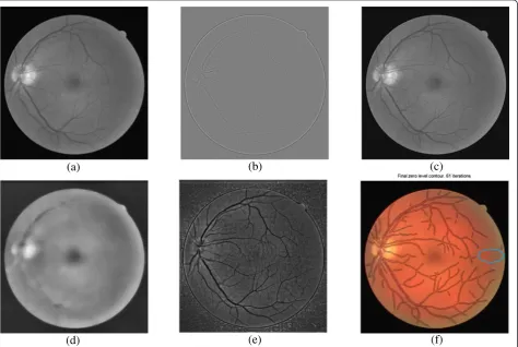
![Figure 12 Preprocessing step and segmentation of non-pathological retinal fundus image obtained from DRIVE dataset.segmented result using only green channel of the histogram-equalized given image based on the proposed structure-based level set segmentationmethod without preprocessing after 61 iterationsonly green channel of the given image based on the proposed structure-based level set segmentation method without preprocessing The smoothedimage using the trace-based approach [39] (a), the image generated by subtracting the original green channel image from the smoothed one(b), the sharpened image [39] (c), the estimated intensity inhomogeneity image obtained by using the median filter (d), the corrected imagebased on our approach (e), segmented image using the proposed structure-based level set segmentation method (f), segmented result using (g), and (h).](https://thumb-us.123doks.com/thumbv2/123dok_us/912519.1589062/12.595.57.538.163.654/preprocessing-segmentation-segmentationmethod-preprocessing-iterationsonly-preprocessing-smoothedimage-inhomogeneity.webp)