https://doi.org/10.1186/s13408-018-0066-8
R E V I E W Open Access
Data Assimilation Methods for Neuronal State and
Parameter Estimation
Matthew J. Moye1·Casey O. Diekman1
Received: 16 February 2018 / Accepted: 11 July 2018 /
© The Author(s) 2018. This article is distributed under the terms of the Creative Commons Attribution 4.0 International License (http://creativecommons.org/licenses/by/4.0/), which permits unrestricted use, distribution, and reproduction in any medium, provided you give appropriate credit to the original author(s) and the source, provide a link to the Creative Commons license, and indicate if changes were made.
Abstract This tutorial illustrates the use of data assimilation algorithms to estimate
unobserved variables and unknown parameters of conductance-based neuronal mod-els. Modern data assimilation (DA) techniques are widely used in climate science and weather prediction, but have only recently begun to be applied in neuroscience. The two main classes of DA techniques are sequential methods and variational meth-ods. We provide computer code implementing basic versions of a method from each class, the Unscented Kalman Filter and 4D-Var, and demonstrate how to use these algorithms to infer several parameters of the Morris–Lecar model from a single volt-age trace. Depending on parameters, the Morris–Lecar model exhibits qualitatively different types of neuronal excitability due to changes in the underlying bifurcation structure. We show that when presented with voltage traces from each of the various excitability regimes, the DA methods can identify parameter sets that produce the correct bifurcation structure even with initial parameter guesses that correspond to a different excitability regime. This demonstrates the ability of DA techniques to per-form nonlinear state and parameter estimation and introduces the geometric structure of inferred models as a novel qualitative measure of estimation success. We conclude by discussing extensions of these DA algorithms that have appeared in the neuro-science literature.
Keywords Data assimilation·Neuronal excitability·Conductance-based models· Parameter estimation
Electronic supplementary material The online version of this article (https://doi.org/10.1186/s13408-018-0066-8) contains supplementary material.
B
C.O. DiekmanM.J. Moye [email protected]
1 Department of Mathematical Sciences & Institute for Brain and Neuroscience Research, New
List of Abbreviations
DA data assimilation
PDE partial differential equation 4D-Var 4D-Variational
EKF Extended Kalman Filter UKF Unscented Kalman Filter SNIC saddle-node on invariant circle EnKF Ensemble Kalman Filter
LETK Local Ensemble Transform Kalman Filter
1 Introduction
1.1 The Parameter Estimation Problem
The goal of conductance-based modeling is to be able to reproduce, explain, and predict the electrical behavior of a neuron or networks of neurons. Conductance-based modeling of neuronal excitability began in the 1950s with the Hodgkin–Huxley model of action potential generation in the squid giant axon [1]. This modeling frame-work uses an equivalent circuit representation for the movement of ions across the cell membrane:
CdV
dt =Iapp−
ion
Iion, (1)
whereV is membrane voltage, C is cell capacitance, Iion are ionic currents, and
Iapp is an external current applied by the experimentalist. The ionic currents arise from channels in the membrane that are voltage- or calcium-gated and selective for particular ions, such sodium (Na+) and potassium (K+). For example, consider the classical Hodgkin–Huxley currents:
INa=gNam3h(V −ENa), (2)
IK=gKn4(V −EK). (3)
The maximal conductancegionis a parameter that represents the density of channels in the membrane. The term(V −Eion)is the driving force, where the equilibrium potentialEionis the voltage at which the concentration of the ion inside and outside of the cell is at steady state. The gating variablemis the probability that one of three identical subunits of the sodium channel is “open”, and the gating variablehis the probability that a fourth subunit is “inactivated”. Similarly, the gating variablenis the probability that one of four identical subunits of the potassium channel is open. For current to flow through the channel, all subunits must be open and not inactivated. The rate at which subunits open, close, inactivate, and de-inactivate depends on the voltage. The dynamics of the gating variables are given by
dx
dt =αx(V )(1−x)+βx(V )x, (4)
The parameters of conductance-based models are typically fit to voltage-clamp recordings. In these experiments, individual ionic currents are isolated using pharma-cological blockers and one measures current traces in response to voltage pulses. However, many electrophysiological datasets consist of current-clamp rather than voltage-clamp recordings. In current-clamp, one records a voltage trace (e.g., a se-ries of action potentials) in response to injected current. Fitting a conductance-based model to current-clamp data is challenging because the individual ionic currents have not been measured directly. In terms of the Hodgkin–Huxley model, only one state variable (V) has been observed, and the other three state variables (m,h, andn) are unobserved. Conductance-based models of neurons often contain several ionic cur-rents and, therefore, more unobserved gating variables and more unknown or poorly known parameters. For example, a model of HVC neurons in the zebra finch has 9 ionic currents, 12 state variables, and 72 parameters [2]. An additional difficulty in attempting to fit a model to a voltage trace is that if one performs a least-squares minimization between the data and model output, then small differences in the tim-ing of action potentials in the data and the model can result in large error [3]. Data assimilation methods have the potential to overcome these challenges by performing state estimation (of both observed and unobserved states) and parameter estimation simultaneously.
1.2 Data Assimilation
Data assimilation can broadly be considered to be the optimal integration of observa-tions from a system to improve estimates of a model output describing that system. Data assimilation (DA) is used across the geosciences, e.g., in studying land hydrol-ogy and ocean currents, as well as studies of climates of other planets [4–6]. An application of DA familiar to the general public is its use in numerical weather pre-diction [7]. In the earth sciences, the models are typically high-dimensional partial differential equations (PDEs) that incorporate dynamics of the many relevant gov-erning processes, and the state system is a discretization of those PDEs across the spatial domain. These models are nonlinear and chaotic, with interactions of system components across temporal and spatial scales. The observations are sparse in time, contaminated by noise, and only partial with respect to the full state-space.
In neuroscience, models can also be highly nonlinear and potentially chaotic. When dealing with network dynamics or wave propagation, the state-space can be quite large, and there are certainly components of the system for which one would not have time course measurements [8]. As mentioned above, if one has a biophys-ical model of a single neuron and measurements from a current-clamp protocol, the only quantity in the model that is actually measured is the membrane voltage. The question then becomes: how does one obtain estimates of the full system state?
To begin, we assume we have a model to represent the system of interest and a way to relate observations we have of that system to the components of the model. Additionally, we allow, and naturally expect, there to be errors present in the model and measurements. To start, let us consider first a general model with linear dynamics and a set of discrete observations which depend linearly on the system components:
yk+1=H xk+1+ηk+1, yk+1∈RM. (6) In this state-space representation,xk is interpreted as the state of the system at some timetk, andyk are our observations. For application in neuroscience, we can take
ML as few state variables of the system are readily observed.F is our model which maps statesxkbetween time pointstk andtk+1.H is our observation operator which describes how we connect our observationsyk+1 to our state-space attk+1. The random variablesωk+1andηk+1represent model error and measurement error, respectively. A simplifying assumption is that our measurements are diluted by Gaus-sian white noise, and that the error in the model can be approximated by GausGaus-sian white noise as well. Thenωk∼N(0, Qk)andηk∼N(0, Rk), whereQkis our model error covariance matrix andRk is our measurement error covariance matrix. We will assume these distributions for the error terms for the remainder of the paper.
We now have defined a stochastic dynamical system where we have characterized the evolution of our states and observations therein based upon assumed error statis-tics. The goal is now to utilize these transitions to construct methods to best estimate the statex over time. To approach this goal, it may be simpler to consider the evalu-ation of background knowledge of the system compared to what we actually observe from a measuring device. Consider the following cost function [9]:
C(x)=1
2y−H x 2 R+
1 2x−x
b2
Pb, (7)
wherez2A=zTA−1z.Pbacts to give weight to certain background componentsxb, andRacts in the same manner to the measurement terms. The model or background term acts to regularize the cost function. Specifically, trying to minimize12y−H x2R
is underdetermined with respect to the observations unless we can observe the full system, and the model term aims to inform the problem of the unobserved compo-nents. We are minimizing over state componentsx. In this way, we balance the influ-ence of what we think we know about the system, such as from a model, compared to what we can actually observe. The cost function is minimized from
∇C=HTR−1H+Pb−1xa−HTR−1y+Pb−1xb=0. (8) This can be restructured as
xa=xb+Ky−H xb, (9)
where
K=PbHTH PbHT +R−1. (10)
The optimal Kalman gain matrix K acts as a weighting of the confidence of our observations to the confidence of our background information given by the model. If the background uncertainty is relatively high or the measurement uncertainty is relatively low,Kis larger, which more heavily weights the innovationy−H xb.
problems resembling the following:
C(x)=1
2 N
k=0
yk−H xk2Rk+ 1 2
N−1 k=0
xk+1−F xk2Pb k
, (11)
where formally the background componentxbhas now been replaced with our model. Now we are concerned with minimizing over an observation window withN+1 time points. Variational methods, specifically “weak 4D-Var”, seek minima of (11) either by formulation of an adjoint problem [10], or directly from numerical optimization techniques.
Alternatively, sequential data assimilation approaches, specifically filters, aim to use information from previous time pointst0, t1, . . . , tk, and observations at the cur-rent timetk+1, to optimally estimate the state attk+1. The classical Kalman filter uti-lizes the form of (10), which minimizes the trace of the posterior covariance matrix of the system at stepk+1,Pka+1, to update the state estimate and system uncertainty. The Kalman filtering algorithm takes the following form. Our analysis estimate, ˆ
xka from the previous iteration, is mapped through the linear model operatorF to obtain our forecast estimatexˆkf+1:
ˆ
xkf+1=Fkxˆka. (12)
The observation operatorH is applied to the forecast estimate to generate the mea-surement estimateyˆkf+1:
ˆ
ykf+1=Hk+1xˆkf+1. (13)
The forecast estimate covariancePkf+1 is generated through calculating the covari-ance from the model and adding it with the model error covaricovari-anceQk:
Pkf+1=FkPkaFkT +Qk. (14)
Similarly, we can construct the measurement covariance estimate by calculating the covariance from our observation equation and adding it to the measurement error covarianceRk:
Pky+1=Hk+1Pkf+1H T
k+1+Rk. (15)
The Kalman gain is defined analogously to (10):
Kk+1=Pkf+1HkT+1
Pky+1−1. (16)
The covariance and the mean estimate of the system are updated through a weighted sum with the Kalman gain:
Pka+1=(I−Kk+1Hk+1)Pkf+1 (17) ˆ
xka+1= ˆxkf+1+Kk+1
yk+1− ˆykf+1
These equations can be interpreted as a predictor–corrector method, where the pre-dictions of the state estimates arexˆkf+1with corresponding uncertaintiesPkf+1in the
forecast. The correction, or analysis, step linearly interpolates the forecast predictions
with observational readings.
In this paper we only consider filters, however smoothers are another form of sequential DA that also use observational data from future timestk+2, . . . , tk+l to estimate the state attk+1.
2 Nonlinear Data Assimilation Methods
2.1 Nonlinear Filtering
For nonlinear models, the Kalman equations need to be adapted to permit nonlinear mappings in the forward operator and the observation operator:
xk+1=f (xk)+ωk+1, ωk∈RL, (19)
yk+1=h(xk+1)+ηk+1, ηk+1∈RM. (20) Our observation operator for voltage data remains linear:h(x)=H x= [e10. . .0]x, where ej is thejth elementary basis vector, is a projection onto the voltage com-ponent of our system. Note thath(x) is an operator, not to be confused with the inactivation gate in (2). Our nonlinear model update, f (x)in (19), is taken as the forward integration of the dynamical equations between observation times.
Multiple platforms for adapting the Kalman equations exist. The most straightfor-ward approach is the extended Kalman filter (EKF) which uses local linearizations of the nonlinear operators in (19)–(20) and plugs these into the standard Kalman equa-tions. By doing so, one preserves Gaussianity of the state-space. Underlying the data assimilation framework is the goal of understanding the distribution, or statistics of the distribution, of the states of the system given the observations:
p(x|y)∝p(y|x)p(x). (21)
The Gaussianity of the state-space declares the posterior conditional distribution
p(x|y)to be a normal distribution by the product of Gaussians being Gaussian, and the statistics of this distribution lead to the Kalman update equations [10]. However, the EKF is really only suitable when the dynamics are nearly linear between obser-vations and can result in divergence of the estimates [11].
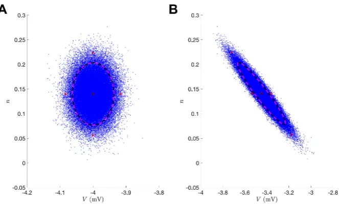
Fig. 1 Unscented transformation. (A) Initial data where blue corresponds to sampling points from a nor-mal distribution of theV , nstate-space and the red circles are the sigma points. Black corresponds to the true uncertainty and mean of the sampled distribution. Magenta corresponds to the statistics of the sigma points. (B) Illustrates the forward operatorf (x)acting on each element of the left panel wheref (x)is the numerical integration of the Morris–Lecar equations (42)–(46) between observation times
some time. The forward operatorf (x)is applied to each of these sigma points, and the mean and covariance of the transformed points can then be computed to estimate the nonlinearly transformed mean and covariance. Figure1depicts this “unscented” transformation. The sigma points precisely estimate the true statistics both initially (Fig.1(A)) and after nonlinear mapping (Fig.1(B)).
In the UKF framework, as with all DA techniques, one is attempting to estimate the states of the system. The standard set of states in conductance-based models includes the voltage, the gating variables, and any intracellular ion concentrations not taken to be stationary. To incorporate parameter estimation, parametersθto be estimated are promoted to states whose evolution is governed by the model error random variable:
θk+1=θk+ωθk+1, ω θ
k∈RD. (22)
This is referred to as an “artificial noise evolution model”, as the random disturbances driving deviations in model parameters over time rob them of their time-invariant definition [12,13]. We found this choice to be appropriate for convergence and as a tuning mechanism. An alternative is to zero out the entries ofQkcorresponding to the parameters in what is called a “persistence model” whereθk+1=θk [14]. However, changes in parameters can still occur during the analysis stage.
We declare our augmented state to be comprised of the states in the dynamical system as well as parametersθof interest:
whereqrepresents the additional states of the system besides the voltage. The filter requires an initial guess of the statexˆ0and covariancePxx. An implementation of this algorithm is provided as Supplementary Material with the parent function UKFML.m and one time step of the algorithm computed in UKF_Step.m.
An ensemble ofσ points are formed and their position and weights are determined byλ, which can be chosen to try to match higher moments of the system distribution [11]. Practically, this algorithmic parameter can be chosen to spread the ensemble for
λ >0, shrink the ensemble for−N < λ <0, or to have the mean point completely removed from the ensemble by setting it to zero. The ensemble is formed on lines 80-82 of UKF_Step.m. The individual weights can be negative, but their cumulative sum is 1.
σPoints: Xj= ˆxka±
(N+λ)Pxx
j, j =1, . . . ,2N, X0= ˆx a k,
Weights: Wj= 1
2(N+λ), j=1, . . . ,2N, W0= λ N+λ.
(24)
We form our background estimatexˆkb+1 by applying our map f (x)to each of the ensemble members
˜
Xj=f (Xj) (25)
and then computing the resulting mean:
Forecast Estimate: xˆkb+1=
2N
j=0
WjX˜j. (26)
We then propagate the transformed sigma points through the observation operator
˜
Yj=h(X˜j) (27)
and compute our predicted observationyˆkb+1from the mapped ensemble:
Measurement Estimate: yˆkb+1=
2N
j=0
WjY˜j. (28)
We compute the background covariance estimate by calculating the variance of the mapped ensemble and adding the process noiseQk:
Background Cov. Est.: Pxxf = 2N
j=0
Wj
˜
Xj− ˆxib+k
˜
Xj− ˆxib+k
T
+Qk (29)
and do the same for the predicted measurement covariance with the addition ofRk:
Predicted Meas. Cov.: Pyy= 2N
j=0
Wj
˜
Yj− ˆykb+1
˜
Yj− ˆykb+1
T
The Kalman gain is computed by matrix multiplication of the cross-covariance:
Cross-Cov.: Pxy= 2N
j=0
Wj
˜
Xj− ˆxkb+1
˜
Yj− ˆykb+1
T
(31)
with the predicted measurement covariance:
Kalman Gain: K=PxyPyy−1. (32) When only observing voltage, this step is merely scalar multiplication of a vector. The gain is used in the analysis, or update step, to linearly interpolate our background statistics with measurement corrections. The update step for the covariance is
Pxxa =Pxxf −KPxyT, (33)
and the mean is updated to interpolate the background estimate with the deviations of the estimated measurement term with the observed datayk+1:
ˆ
xka+1= ˆxkb+1+Kyk+1− ˆykb+1
. (34)
The analysis step is performed on line 124 of UKF_Step.m. Some implementa-tions also include a redistribution of the sigma points about the forecast estimate using the background covariance prior to computing the cross-covariancePxyor the predicted measurement covariancePyy [15]. So, after (29), we redefineX˜j, Y˜j in (25) as follows:
˜
Xj= ˆxbk+1±
(N+λ)Pxx
j, j=1, . . . ,2N, ˜
Yj=h(X˜j).
The above is shown in lines 98–117 in UKF_Step. A particularly critical part of us-ing a filter, or any DA method, is choosus-ing the process covariance matrixQkand the measurement covariance matrixRk. The measurement noise may be intuitively based upon knowledge of one’s measuring device, but the model error is practically impos-sible to know a priori. Work has been done to use previous innovations to simul-taneously estimateQandR during the course of the estimation cycle [16], but this becomes a challenge for systems with low observability (such as is the case when only observing voltage). Rather than estimating the states and parameters simultaneously as with an augmented state-space, one can try to estimate the states and parameters separately. For example, [17] used a shooting method to estimate parameters and the UKF to estimate the states. This study also provided a systematic way to estimate an optimal covariance inflationQk. For high-dimensional systems where computational efficiency is a concern, an implementation which efficiently propagates the square root of the state covariance has been developed [18].
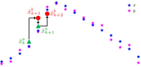
Fig. 2 Example of iterative estimation in UKF. The red circles are the result of forward integration through the model using the previous best estimates. The green are the estimates after combining these with obser-vational data. The blue stars depict the true system output (without any noise), and the magenta stars are the noisy observational data with noise generated by (48) andε=0.1
2.2 Variational Methods
In continuous time, variational methods aim to find minimizers of functionals which represent approximations to the probability distribution of a system conditioned on some observations. As our data is available only in discrete measurements, it is prac-tical to work with a discrete form similar to (7) for nonlinear systems:
C(x)=1
2 N
k=0
yk−h(xk) 2 Rk+
1 2
N−1 k=0
xk+1−f (xk) 2
Pkb. (35)
We assume that the states follow the state-space description in (19)–(20) with
ωk∼N(0, Q)andηk∼N(0, R), whereQis our model error covariance matrix and
Ris our measurement error covariance matrix. As an approximation, we imposeQ,R
to be diagonal matrices, indicating that there is assumed to be no correlation between errors in other states. Namely,Q, contains only the assumed model error variance for each state-space component, andRis just the measurement error variance of the voltage observations. These assumptions simplify the cost function to the following:
C(x)=1
2 N
k=0
R−1(yk−Vk)2+ 1 2
L
l=1 N−1
k=0
Q−l,l1xl,k+1−fl(xk)
2
, (36)
whereVk=x1,k. For the current-clamp data problem in neuroscience, one seeks to minimize equation (36) in what is called the “weak 4D-Var” approach. An example implementation of weak 4D-Var is provided in w4DvarML.m in the Supplementary Material. An example of the cost function with which to minimize over is given in the child function w4dvarobjfun.m. Each of thexk is mapped byf (x)on line 108. Alternatively, “strong 4D-Var” forces the resulting estimates to be consistent with the modelf (x). This can be considered the result of takingQ→0, which yields the
nonlinearly constrained problem
C(x)=1
2 N
k=0
such that
xk+1=f (xk), k=0, . . . , N. (38)
The rest of this paper will be focused on the weak case (36), where we can define the argument of the optimization as follows:
x= [x1,1, x1,2, . . . , x1,N, x2,1, . . . , xL,N, θ1, θ2, . . . , θD] (39) resulting in an(N+1)L+D-dimensional estimation problem. An important aspect of the scalability of this problem is that the Hessian matrix
Hi,j=
∂2C ∂xi∂xj
(40)
is sparse. Namely, each state at each discrete time has dependencies based upon the model equations and the chosen numerical integration scheme. At the heart of many gradient-based optimization techniques lies a linear system, involving the Hessian and the gradient∇C(xn)of the objective function, that is used to solve for the next candidate point. Specifically, Newton’s method for optimization is
xn+1=xn−H−1∇C(xn). (41)
Therefore, if(N+1)L+D is large, then providing the sparsity pattern is advan-tageous when numerical derivative approximations, or functional representations of them, are being used to perform minimization with a derivative-based method. One can calculate these derivatives by hand, symbolic differentiation, or automatic differ-entiation.
A feature of the most common derivative-based methods is assured convergence to local minima. However, our problem is non-convex due to the model term, which leads to the development of multiple local minima in the optimization surface as de-picted in Fig.3. For the results in this tutorial, we will only utilize local optimization tools, but see Sect.5for a brief discussion of some global optimization methods with stochastic search strategies.
3 Application to Spiking Regimes of the Morris–Lecar Model
3.1 Twin Experiments
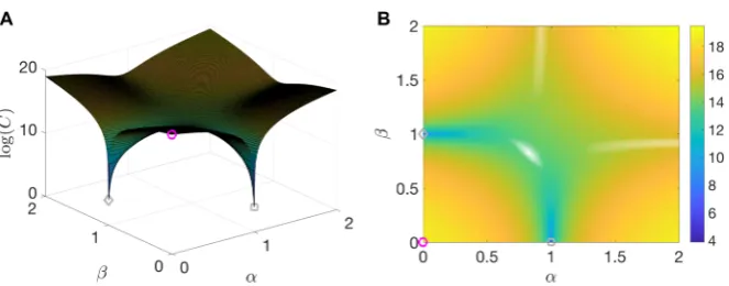
Fig. 3 Example cost function for 4D-Var. (A) Surface generated by taking the logarithm ofC(α, β), whereC(α, β)=C(x0(1−α)(1−β)+αxmin,d+βxmin,s)so that atα=β=0, x=x0(magenta circle),
and atα=1 andβ=0, x=xmin,dfor the deeper minima (gray square), and similarly for the shallower
minima (gray diamond). (B) Contour plot of the surface shown in (A)
Before applying a method to data from a real biological experiment, it is important to test it against simulated data where the ground truth is known. In these experiments, one creates simulated data from a model and then tries to recover the true states and parameters of that model from the simulated data alone.
3.2 Recovery of Bifurcation Structure
In conductance-based models, as well as in real neurons, slight changes in a parame-ter value can lead to drastically different model output or neuronal behavior. Sudden changes in the topological structure of a dynamical system upon smooth variation of a parameter are called bifurcations. Different types of bifurcations lead to different neuronal properties, such as the presence of bistability and subthreshold oscillations [23]. Thus, it is important for a neuronal model to accurately capture the bifurca-tion dynamics of the cell being modeled [24]. In this paper, we ask whether or not the models estimated through data assimilation match the bifurcation structure of the model that generated the data. This provides a qualitative measure of success or failure for the estimation algorithm. Since bifurcations are an inherently nonlinear phenomenon, our use of topological structure as an assay emphasizes how nonlinear estimation is a fundamentally distinct problem from estimation in linear systems.
3.3 Morris–Lecar Model
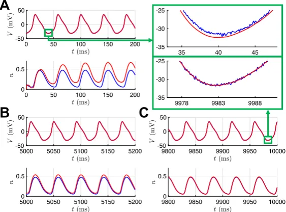
Fig. 4 Three different excitability regimes of the Morris–Lecar model. The bifurcation diagrams in the top row depict stable fixed points (red), unstable fixed points (black), stable limit cycles (blue), and unstable limit cycles (green). Gray dots indicate bifurcation points, and the dashed gray lines indicate the value of Iappcorresponding to the traces shown forV(middle row) andn(bottom row). (A) AsIappis increased
from 0 or decreased from 250 nA, the branches of stable fixed points lose stability through subcritical Hopf bifurcation, and unstable limit cycles are born. The branch of stable limit cycles that exists atIapp=100
nA eventually collides with these unstable limit cycles and is destroyed in a saddle-node of periodic orbits (SNPO) bifurcation asIappis increased or decreased from this value. (B) AsIappis increased from 0,
a branch of stable fixed points is destroyed through saddle-node bifurcation with the branch of unstable fixed points. AsIappis decreased from 150 nA, a branch of stable fixed points loses stability through
subcritical Hopf bifurcation, and unstable limit cycles are born. The branch of stable limit cycles that exists atIapp=100 nA is destroyed through a SNPO bifurcation asIappis increased and a SNIC bifurcation
asIappis decreased. (C) Same as (B), except that the stable limit cycles that exist atIapp=36 nA are
destroyed through a homoclinic orbit bifurcation asIappis decreased
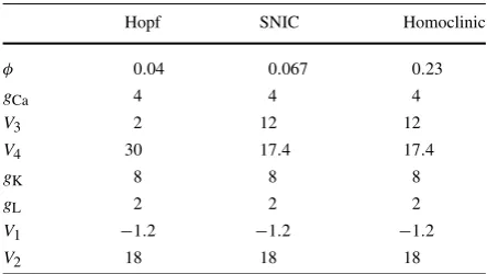
Table 1 Morris–Lecar parameter values. For all simulations,C=20, ECa=120,EK= −84, and
EL= −60. For the Hopf and
SNIC regime,Iapp=100; for
the homoclinic regime, Iapp=36
Hopf SNIC Homoclinic
φ 0.04 0.067 0.23
gCa 4 4 4
V3 2 12 12
V4 30 17.4 17.4
gK 8 8 8
gL 2 2 2
V1 −1.2 −1.2 −1.2
V2 18 18 18
The equations for the Morris–Lecar model are as follows:
Cm
dV
dt =Iapp−gL(V −EL)−gKn(V −EK)
−gCam∞(V )(V−ECa)
=fV(V , n;θ), (42)
dn dt =φ
n∞(V )−n/τn(V )=fn(V , n;θ), (43)
with
m∞=1
2
1+tanh(V−V1)/V2
, (44)
τn=1/cosh
(V−V3)/2V4
, (45)
n∞=1
2
1+tanh(V−V3)/V4
. (46)
The eight parameters that we will attempt to estimate from data aregL,gK,gCa,
φ,V1,V2,V3, andV4. We are interested in whether the estimated parameters yield a model with the desired mechanism of excitability. Specifically, we will conduct twin experiments where the observed data is produced by a model with parameters in a certain bifurcation regime, but the data assimilation algorithm is initialized with parameter guesses corresponding to a different bifurcation regime. We then assess whether or not a model with the set of estimated parameters undergoes the same bifurcations as the model that produced the observed data. This approach provides an additional qualitative measure of estimation accuracy, beyond simply comparing the values of the true and estimated parameters.
3.4 Results with UKF
The UKF was tested on the Morris–Lecar model in an effort to simultaneously esti-mateV andnalong with the eight parameters in Table1. Data was generated via a modified Euler scheme at observation points every 0.1 ms, where we take the step-sizetas 0.1 as well:
˜
xk+1=xk+tf(tk, xk),
xk+1=xk+
t
2
f(tk, xk)+f(tk+1,x˜k+1)
=f (xk).
(47)
function fXaug.m, provided in the Supplementary Material, represents our augmented vector field. Our observational operatorH is displayed on line 136 of UKFML.m. To reiterate, the states to be estimated in the Morris–Lecar model are the voltage and the potassium gating variable. The eight additional parameters are promoted to the mem-bers of state-space with trivial dynamics resulting in a ten-dimensional estimation problem.
These examples were run using 20 seconds of data which is 200,001 time points. During this time window, the Hopf, SNIC, and homoclinic models fire 220, 477, and 491 spikes, respectively. Such a computation for a ten-dimensional model takes only a few minutes on a laptop computer.Rcan be set to 0 when one believes the observed signal to be completely noiseless, but even then it is commonly left as a small num-ber to try to mitigate the development of singularities in the predicted measurement covariance. We set our observed voltage to be the simulated output using modified Euler with additive white noise at each time point:
Vobs(t )=Vtrue(t )+η(t ), (48)
whereη∼N(0, (εσtrue)2)is a normal random variable whose variance is equal to the square of the standard deviation of the signal scaled by a factorε, which is kept fixed at 0.01 for these simulations.Ris taken as the variance ofη. The initial covariance of the system isαII, whereIis the identity matrix andαIis 0.001. The initial guess forn is taken to be 0.Qis fixed in time as a diagonal matrix with diagonal 10−7 [max(Vobs)−min(Vobs),1,|θ0|], whereθ0 represents our initial parameter guesses. We setλ=5; however, this parameter was not especially influential for the results of these runs, as discussed further below. These initializations are displayed in the body of the parent function UKFML.m.
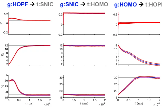
Figure5shows the state estimation results when the observed voltage is from the SNIC regime, but the UKF is initialized with parameter guess corresponding to the Hopf regime. Initially, the state estimate fornand its true, unobserved dynamics have great disparity. As the observations are assimilated over the estimation window, the states and model parameters adjust to produce estimates which better replicate the observed, and unobserved, system components. In this way, information from the observations is transferred to the model. The evolution of the parameter estimates for this case is shown in the first column of Fig.6, withφ,V3, and V4 all converging to close to their true values after 10 seconds of observations. The only difference in parameter values between the SNIC and homoclinic regimes is the value of the parameterφ. The second column of Fig.6shows that when the observed data is from the homoclinic regime but the initial parameter guesses are from the SNIC regime, the estimates ofV3 andV4remain mostly constant near their original (and correct) values, whereas the estimate ofφquickly converges to its new true value. Finally, the third column of Fig.6shows that all three parameter estimates evolve to near their true values when the UKF is presented with data from the Hopf regime but initial parameter estimates from the homoclinic regime.
Fig. 5 State estimates for UKF. This example corresponds to initializing with parameters from the HOPF regime and attempting to correctly estimate those of the SNIC regime. The noisy observed voltageV and true unobserved gating variablenare shown in blue, and their UKF estimates are shown in red
Table 2 UKF parameter estimates at end of estimation window, with observed data from bifurcation regime ‘t’ and initial parameter guesses corresponding to bifurcation regime ‘g’
t:HOPF t:SNIC t:HOMO
g:HOPF g:SNIC g:HOMO g:HOPF g:SNIC g:HOMO g:HOPF g:SNIC g:HOMO φ 0.040 0.40 0.040 0.067 0.040 0.067 0.237 0.224 0.224 gCa 4.017 4.019 4.025 4.001 4.000 4.001 4.112 3.874 3.877
V3 1.612 1.762 1.660 11.931 11.937 11.912 11.751 11.784 11.772
V4 29.646 29.832 29.771 17.343 17.337 17.342 17.739 16.806 16.815
gK 7.895 7.926 7.892 7.970 7.971 7.958 7.929 7.854 7.850
gL 2.032 2.027 2.033 2.003 2.004 2.003 2.025 1.967 1.968
V1 −1.199 −1.195 −1.189 −1.193 −1.193 −1.190 −1.064 −1.346 −1.341
V2 18.045 18.053 18.067 17.991 17.991 17.991 18.179 17.734 17.740
model. To assess the inferred models, we generate bifurcation diagrams using the es-timated parameters and compare them to the bifurcation diagrams for the parameters that produced the observed data. Figure7shows that the SNIC and homoclinic bifur-cation diagrams were recovered quite exactly. The Hopf structure was consistently recovered, but with shifted regions of spiking and quiescence and minor differences in spike amplitude.
Fig. 6 Parameter estimates for UKF. This example corresponds to initializing with parameters from the HOPF, SNIC, and HOMO regimes and attempting to correctly estimate those of the SNIC, HOMO, and HOPF regimes (left to right column, respectively). The blue curves are the estimates from the UKF, with
±2 standard deviations from the mean (based on the filter estimated covariance) shown in red. The gray lines indicate the true parameter values
Fig. 7 Bifurcation diagrams for UKF twin experiments. The gray lines correspond to the true diagrams, and the blue dotted lines correspond to the diagrams produced from the estimated parameters in Table2
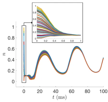
Fig. 8 UKF state estimates ofn for the Morris–Lecar model with 100 different initial guesses of the state sampled fromU(0,1), with all other parameters held fixed
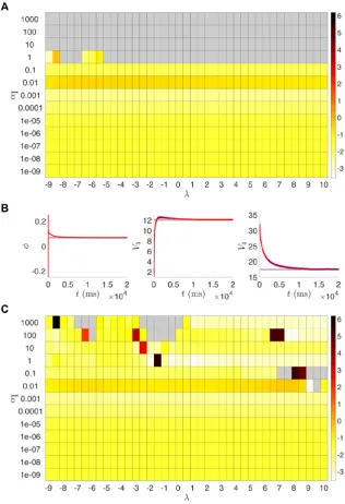
paper, we always initialized the UKF with initial parameter values corresponding to the various bifurcation regimes and did not explore the performance for randomly selected initial parameter guesses. For initial parameter guesses that are too far from the true values, it is possible that the filter would converge to incorrect parameter val-ues or fail outright before reaching the end of the estimation window. Additionally, we investigated the choices of certain algorithmic parameters for the UKF, namelyλ
andαI. Figure9(A) shows suitable ranges of these parameters, with the color indi-cating the root mean squared error of the parameters at the end of the cycle compared to their true values. We found this behavior to be preserved across our nine twin ex-periment scenarios. Notably, this shows that our results in Table2were generated using an initial covarianceαI=0.001 that was smaller than necessary. By increasing the initial variability, the estimated system can converge to the true dynamics more quickly, as shown forαI=0.1 in Fig.9(B). The value ofλdoes not have a large im-pact on these results, except for whenαI=1. Here the filter fails before completing the estimation cycle, except for a few cases whereλis small enough to effectively shrink the ensemble spread and compensate for the large initial covariance. For ex-ample, withλ= −9, we haveN−9=1 and, therefore, the ensemble spread in (24) is simplyXj = ˆxka±
√
Fig. 9 (A) UKF results from runs of the t:SNIC/g:HOPF twin experiment for various parameter combi-nations ofλandαI. The color scale represents the root mean squared error of the final parameter values atT =200,001 from the parameters of the SNIC bifurcation regime. Gray indicates the filter failed out-right before reaching the end of the estimation window. (B) Parameter estimates over time for the run withλ=5, αI=0.1. The parameters (especiallyφandV3) approach their true values more quickly than
modified Euler method (47) before proceeding can enable the filter to reach the end of the estimation window and yield reasonable parameter estimates.
3.5 Results with 4D-Var
The following results illustrate the use of weak 4D-Var. One can minimize the cost function (36) using a favorite choice of optimization routine. For the following ex-amples, we will consider a local optimizer by using interior point optimization with MATLAB’s built-in solver fmincon. At the heart of the solver is a Newton-step which uses information about the Hessian, or a conjugate gradient step using gradient in-formation [27–29]. The input we are optimizing over conceptually takes the form of
x= [V0, V1, . . . , VN, n0, n1, . . . , nN, θ1, θ2, . . . , θD] (49) resulting in an(N+1)L+D-dimensional estimation problem whereL=2. There are computational limitations with memory storage and the time required to suffi-ciently solve the optimization problem to a suitable tolerance for reasonable parame-ter estimates. Therefore, we cannot be cavalier with using as much data with 4D-Var as we did with the UKF, as that would result in a(200,001)2+8=400,010 dimen-sional problem. Using Newton’s method (41) on this problem would involve inverting a Hessian matrix of size(400,010)2, which according to a rough calculation would require over 1 TB of RAM. Initialization of the optimization is shown on line 71 of
w4DVarML.m.
The estimated parameters are given in Table 3. These results were run using
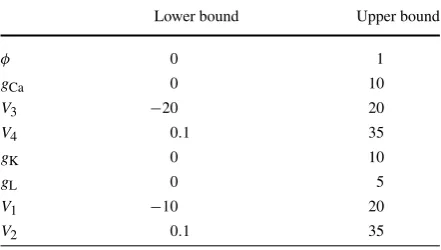
N=2001 time points. To simplify the search space, the parameter estimates were constrained between the bounds listed in Table4. These ranges were chosen to en-sure that the maximal conductances, the rateφ, and the activation curve slopeV2all remain positive. We found that running 4D-Var with even looser bounds (TableA1) yielded less accurate parameter estimates (TablesA2andA3). The white noise per-turbations for the 4D-Var trials were the same as those from the UKF examples. Initial guesses for the states at each time point are required. For these trials,V is ini-tialized asVobs, andnis initialized as the result of integration of its dynamics forced withVobsusing the initial guesses for the parameters, i.e.,n= fn(Vobs, n;θ0). The initial guesses are generated beginning on line 38 of w4DvarML.m. We impose that
Q−1in (36) is a diagonal matrix with entriesαQ[1,1002]to balance the dynamical variance ofV andn. The scaling factorαQrepresents the relative weight of the model term compared to the measurement term. Based on preliminary tuning experiments, we setαQ=100 for the results presented.
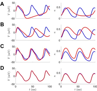
Fig. 10 Example of 4D-Var assimilation initializing with parameters from the Hopf regime but observa-tional data from the SNIC regime. The blue traces are noiseless versions of the observed voltage data (left column) or the unobserved variablen(right column) from the model that produced the data. The red traces are the result of integrating the model with the estimated parameter sets at various points during the course of the optimization. (A) Initial parameter guesses. (B) Parameter values after 100 iterations. C: Parameter values after 1000 iterations. D: Parameter values after 30,000 iterations (corresponds to t:SNIC/g:HOPF column of Table3)
Table 3 4D-Var parameter estimates at the end of the optimization for each bifurcation regime. The pa-rameter bounds in Table4were used for these trials. Hessian information was not provided to the optimizer
t:HOPF t:SNIC t:HOMO
g:HOPF g:SNIC g:HOMO g:HOPF g:SNIC g:HOMO g:HOPF g:SNIC g:HOMO φ 0.040 0.037 0.039 0.069 0.067 0.066 0.414 0.218 0.230 gCa 4.000 3.890 3.976 4.024 4.000 4.045 9.037 3.813 3.999
V3 2.000 3.404 3.241 12.695 12.000 12.076 7.458 13.022 12.004
V4 30.000 29.085 30.122 18.759 17.400 16.990 28.365 17.165 17.403
gK 8.000 8.386 8.287 8.284 8.000 8.009 9.817 8.472 8.002
gL 2.000 2.016 2.021 1.930 2.000 2.071 3.140 1.941 2.000
V1 −1.200 −1.335 −1.250 −1.078 −1.200 −1.179 2.872 −1.419 −1.202
V2 18.000 17.619 17.911 18.091 18.000 18.162 24.769 17.712 18.000
Table 4 Bounds used during 4D-Var estimation for the results
shown in Tables3andA4 Lower bound Upper bound
φ 0 1
gCa 0 10
V3 −20 20
V4 0.1 35
gK 0 10
gL 0 5
V1 −10 20
V2 0.1 35
A drawback of the results shown in Table3 is that for the default tolerances in
fmincon, some runs took more than two days to complete on a dedicated core.
Fig. 11 Example parameter estimation with 4D-Var initializing with Hopf parameter regime and estimat-ing parameters of SNIC regime
Fig. 12 Bifurcation diagrams for 4D-Var twin experiments. The gray lines correspond to the true dia-grams, and the blue dotted lines correspond to the diagrams produced from the estimated parameters in Table3
estimated simultaneously. A tutorial specific to collocation methods for optimization has been developed [31].
Fig. 13 (A) Sparsity pattern for the Hessian of the cost function for the Morris–Lecar equations for N+1=2001 time points. The final eight rows (and symmetrically the last eight columns) depict how the states at each time depend upon the parameters. (B) The top left corner of the Hessian shown in (A)
Fig. 14 (A) Logarithm of the value of the cost function for a twin experiment initialized with parameters from the Hopf regime but observational data from the SNIC regime. The iterates were generated from
fmincon with provided Hessian and gradient functions. (B) Bifurcation diagrams produced from parameter
estimates for selected iterations. The blue is the initial bifurcation structure, the gray is the true bifurcation structure for the parameters that generated the observed data, the red is the bifurcation structure of the iterates, and the green is the bifurcation structure of the optimal point determined by fmincon
Again, these results, at best, can reflect only locally optimal solutions of the op-timization manifold. The 4D-Var framework has been applied to neuroscience using a more systematic approach to finding the global optimum. In [32], a population of initial states x is optimized in parallel with an outer loop that incorporates an
anneal-ing algorithm. The annealanneal-ing parameter relates the weights of the two summations
in (36), and the iteration proceeds by increasing the weight given to the model error compared to the measurement error.
We also wished to understand more about the sensitivity of this problem to initial conditions. We initialized the system with the voltage states as those of the obser-vation, the parameters as those of the initializing guess bifurcation regime, and the gating variable[n0, n1, . . . nN]to be i.i.d. fromU(0,1). The results confirm our sus-picions that multiple local minima exist. For 100 different initializations ofn, for the problem of going from SNIC to HOPF, 63 were found to fall into a deeper minima, yielding better estimates and a smaller objective function value, while 16 fell into a shallower minima, and the rest into three different even shallower minima. While one cannot truly visualize high-dimensional manifolds, one can try to visualize a subset of the surface. Figure3shows the surface that arises from evaluating the objective function on a linear combination of the two deepest minima and an initial condition
x0, which eventually landed in the shallower of the two minima as points in 4010-dimensional space.
4 Application to Bursting Regimes of the Morris–Lecar Model
Many types of neurons display burst firing, consisting of groups of spikes separated by periods of quiescence. Bursting arises from the interplay of fast currents that gen-erate spiking and slow currents that modulate the spiking activity. The Morris–Lecar model can be modified to exhibit bursting by including a calcium-gated potassium (KCa) current that depends on slow intracellular calcium dynamics [33]:
Cm
dV
dt =Iapp−gL(V −EL)−gKn(V−EK)
−gCam∞(V )(V−ECa)−gKCaz(V −EK), (50)
dn dt =φ
n∞(V )−n/τn(V ), (51)
dCa
dt =ε(−μICa−Ca), (52)
z= Ca
Ca+1. (53)
Table 5 Parameters for bursting in the modified Morris–Lecar model. For square-wave burstingIapp=45,
and for elliptic bursting Iapp=120. All other parameters
are the same as in Table1
Square-wave Elliptic
φ 0.23 0.04
gCa 4 4.4
V3 12 2
V4 17.4 30
gK 8 8
gL 2 2
V1 −1.2 −1.2
V2 18 18
gKCa 0.25 0.75
ε 0.005 0.005
μ 0.02 0.02
orbits bifurcation. The voltage traces produced by these two types of bursting are quite distinct, as shown in Fig.15.
4.1 Results with UKF
We conducted a set of twin experiments for the bursting model to address the same question as we did for the spiking model: from a voltage trace alone, can DA meth-ods estimate parameters that yield the appropriate qualitative dynamical behavior? Specifically, we simulated data from the square-wave (elliptic) bursting regime, and then initialized the UKF with parameter guesses corresponding to elliptic (square-wave) bursting (these parameter values are shown in Table5). As a control experi-ment, we also ran the UKF with initial parameter guesses corresponding to the same bursting regime as the observed data. The observed voltage trace included additive white noise generated following the same protocol as in previous trials. We used 200,001 time points with observations at every 1 ms. Between observations, the sys-tem was integrated forward using substeps of 0.025 ms. For the square-wave burster, this included 215 bursts with 4 spikes per burst, and 225 bursts with 2 spikes for the elliptic burster.
Table 6 UKF parameter estimates for each bursting
regime t:Square-wave t:Elliptic
g:Square-wave g:Elliptic g:Square-wave g:Elliptic
φ 0.214 0.215 0.040 0.040
gCa 3.758 3.767 4.396 4.398
V3 12.045 12.023 1.603 1.685
V4 16.272 16.316 29.582 29.639
gK 7.955 7.952 7.866 7.889
gL 1.974 1.972 2.015 2.017
V1 −1.514 −1.511 −1.120 −1.199
V2 17.640 17.624 18.010 18.015
gKCa 0.251 0.251 0.767 0.763
Fig. 16 Bifurcation diagrams for UKF twin experiments for the bursting Morris–Lecar model. The gray lines correspond to the true diagrams, and the blue dotted lines correspond to the diagrams produced from the estimated parameters in Table6
Table 7 4D-Var parameter estimates for each bursting
regime t:Square-wave t:Elliptic
g:Square-wave g:Elliptic g:Square-wave g:Elliptic
φ 0.230 0.260 0.037 0.040
gCa 4.009 4.509 4.244 4.412
V3 12.009 11.920 6.667 1.971
V4 17.437 19.581 32.605 30.026
gK 8.006 8.244 9.485 8.002
gL 2.003 2.068 1.979 2.009
V1 −1.187 −0.627 −1.307 −1.172
V2 18.029 18.754 17.469 18.049
gKCa 0.250 0.237 0.554 0.741
4.2 Results with 4D-Var
We also investigated the utility of variational techniques to recover the mechanisms of bursting. For these runs, we took our observations to be coarsely sampled at 0.1 ms, and our forward mapping is taken to be one step of modified Euler between ob-servation times, as was the case for our previous 4D-Var Morris–Lecar results. We used 10,000 time points, which is one burst for the square wave burster, and one full burst plus another spike for the elliptic burster. We used the L-BFGS-B method [35], as we found it to perform faster for this problem than fmincon. This method approxi-mates the Broyden–Fletcher–Goldfarb–Shanno (BFGS) quasi-Newton algorithm us-ing a limited memory (L) inverse Hessian approximation, with an extension to handle bound constraints (B). It is available for Windows through the OPTI toolbox [36] or through a nonspecific operating system MATLAB MEX wrapper [37]. We supplied the gradient of the objective function, but allowed the solver to define the limited-memory Hessian approximation for our 30,012-dimensional problem. The results are captured in Table7. We performed the same tests with providing the Hessian; how-ever, there was no significant gain in accuracy or speed. The value forgKCafor ini-tializing with the square wave parameters and estimating the elliptical parameters is quite off, which reflects our earlier assessment for the value in observing calcium dy-namics. Figure17shows that we are still successful in recovering the true bifurcation structure.
5 Discussion and Conclusions
Fig. 17 Bifurcation diagrams for 4D-Var twin experiments for the bursting Morris–Lecar model. The gray lines correspond to the true diagrams, and the blue dotted lines correspond to the diagrams produced from the estimated parameters in Table7
We showed the effectiveness of standard implementations of the Unscented Kalman Filter and weak 4D-Var to recover spiking behavior and, in many circum-stances, near-exact parameters of interest. We showed that the estimated models un-dergo the same bifurcations as the model that produced the observed data, even when the initial parameter guesses do not. Additionally, we are also provided with esti-mates of the states and uncertainties associated with each state and parameter, but for sake of brevity these values were not always displayed. The methods, while not insensitive to noise, have intrinsic weightings of measurement deviations to account for the noise of the observed signal. Results were shown for mild additive noise. We also extended the Morris–Lecar model to exhibit bursting activity and demonstrated the ability to recover these model parameters using the UKF.
Table 8 Comparison of the sequential (UKF) and variational (4D-Var) approaches to data assimilation
UKF 4D-Var
Implementation choices initial covariance (Pxx) model uncertainty (Q−1) sigma points (λ) type of optimizer/optimizer settings process covariance matrix (Q) state and parameter bounds Data requirements Pro: can handle a large amount of
data
Pro: may find a good solution with a small amount of data
Con: may not find a good solution with a small amount of data
Con: cannot handle a large amount of data
Run time Minutes Days, hours, or minutes depending
on choice of optimizer and settings Scalability to larger models Harder to choose Q Search dimension is(N+1)L+D
EnKF may use a smaller number of ensemble members
Sparse Hessian can be exploited during optimization
time. There are natural ways to provide parameter bounds in the 4D-Var framework, whereas this is not the case for the UKF. However, depending upon the implemen-tation choices and the dimension of the problem (which is extremely large for long time series data), the optimization may take a computing time scale of days to yield reasonable estimates. Fortunately, derivative information can be provided to the op-timizer to speed up the 4D-Var procedure. Both the UKF and 4D-Var can provide estimates of the system uncertainty in addition to estimates of the system mean. The UKF provides mean and variance estimates at each iteration during the analysis step. In 4D-Var, one seeks mean estimates by minimization of a cost function. It has been shown that for cost functions of the form (36), the system variance can be interpreted as the inverse of the Hessian evaluated at minima of (36), and scales roughly asQ
for largeQ−1[32]. The pros and cons of implementing these two DA approaches are summarized in Table8.
The UKF and 4D-Var methodologies welcome the addition of any observables of the system, but current-clamp data may be all that is available. With this experimental data in mind, for a more complex system, the number of variables increases, while the total number of observables will remain at unity. Therefore, it may be useful to assess a priori which parameters are structurally identifiable and the sensitivity of the model to parameters of interest in order to reduce the estimation state-space [38]. Additionally, one should consider what manner of applied current to use to aid in state and parameter estimation. In the results presented above, we used a constant applied current, but work has been done which suggests the use of complex time-varying currents that stimulate as many of the model’s degrees of freedom as possible [39].
on real data from pyramidal neurons to track the states and externally applied current [43], the connectivity of cultured neuronal networks sampled by a microelectrode ar-ray [44], to assimilate seizure data from hippocampal OLM interneurons [15], and to reconstruct mammalian sleep dynamics [17]. A comparative study of the efficacy of the EKF and UKF on conductance-based models has been conducted [45].
The UKF is a particularly good framework for the state dimensions of a single compartment conductance based model as the size of the ensemble is chosen to be 2(L+D)+1. When considering larger state dimensions, as is the case for PDE models, a more general Ensemble Kalman Filter (EnKF) may be appropriate. An in-troduction to the EnKF can be found in [46,47]. An adaptive methodology using past innovations to iteratively estimate the model and measurement covariancesQandR
has been developed for use with ensemble filters [16]. The Local Ensemble Tranform Kalman Filter (LETKF) [48] has been used to estimate the states associated with car-diac electrical wave dynamics [8]. Rather than estimating the mean and covariance through an ensemble, particle filters aim to fully construct the posterior density of the states conditioned on the observations. A particle filter approach has been applied to infer parameters of a stochastic Morris–Lecar model [49], to assimilate spike train data from rat layer V cortical neurons into a biophysical model [50], and to assimilate noisy, model-generated data for other states to motivate the use of imaging techniques when available [51].
An approach to the variational problem which tries to uncover the global minima more systematically has been developed [32]. In this framework, comparing to (36), they define for diagonal entries ofQ−1that
Q−1=Q−01αβ
forα >1 andβ≥0. The model term is initialized as relatively small, and over the course of an annealing procedure,β is incremented resulting in a steady increase of the model term’s influence on the cost function. This annealing schedule is conducted in parallel for different initial guesses for the state-space. The development of this variational approach can be found in [52], and it has been used to assimilate neuronal data from HVC neurons [34] as well as to calibrate a neuromorphic very large scale integrated (VLSI) circuit [53]. An alternative to the variational approach is to frame the assimilation problem from a probabilistic sampling perspective and use Markov chain Monte-Carlo methods [54].
A closely associated variational technique, known as “nudging”, augments the vector field with a control term. If we only have observations of the voltage, this manifests as follows:
dV dt =f
V(V ,q;θ)+u(Vobs−V ).
prob-lem often encountered when fitting models to a voltage trace is that phase shifts, or small differences in spike timing, between model output and the data can result in large root mean square error. This is less of an issue for data assimilation methods, especially sequential algorithms like UKF. Other approaches to avoid harshly penal-izing spike timing errors in the cost function are to consider spikes in the data and model-generated spikes that occur within a narrow time window of each other as co-incident [60], or to minimize error with respect to thedV /dtversusV phase–plane trajectory rather thanV (t )itself [59]. Another way to avoid spike mismatch errors is to force the model with the voltage data and perform linear regression to estimate the linear parameters (maximal conductances), and then perhaps couple the problem with another optimization strategy to access the nonlinearly-dependent gating parameters [3,61,62].
A common optimization strategy is to construct an objective function that en-capsulates important features derived from the voltage trace, and then use a genetic algorithm to stochastically search for optimal solutions. These algorithms proceed by forming a population of possible solutions and applying biologically inspired evolu-tion strategies to gradually increase the fitness (defined with respect to the objective function) of the population across generations. Multi-objective optimization schemes will generate a “Pareto front” of optimal solutions that are considered equally good. A multi-objective non-dominated sorting genetic algorithm (NSGA-II) has recently been used to estimate parameters of the pacemaker PD neurons of the crab pyloric network [63,64].
In this paper, we compared the bifurcation structure of models estimated by DA algorithms to the bifurcation structure of the model that generated the data. We found that the estimated models exhibited the correct bifurcations even when the algorithms were initiated in a region of parameter space corresponding to a different bifurcation regime. This type of twin experiment is a useful addition to the field that specifically emphasizes the difficulty of nonlinear estimation and provides a qualitative measure of estimation success or failure. Prior literature on parameter estimation that has made use of geometric structure includes work on bursting respiratory neurons [65] and “inverse bifurcation analysis” of gene regulatory networks [66,67].
Looking forward, data assimilation can complement the growth of new recording technologies for collecting observational data from the brain. The joint collabora-tion of these automated algorithms with the painstaking work of experimentalists and model developers may help answer many remaining questions about neuronal dynamics.
Acknowledgements We thank Tyrus Berry and Franz Hamilton for helpful discussions about the UKF and for sharing code, and Nirag Kadakia and Paul Rozdeba for helpful discussions about 4D-Var methods and for sharing code. MM also benefited from lectures and discussions at the Mathematics and Climate Summer Graduate Program held at the University of Kansas in 2016, which was sponsored by the Institute for Mathematics and its Applications and the Mathematics and Climate Research Network.
Availability of data and materials The MATLAB code used in this study is provided as Supplementary Material.
Ethics approval and consent to participate Not applicable.
Competing interests The authors declare that they have no competing interests. Consent for publication Not applicable.
Authors’ contributions MM wrote the computer code implementing the data assimilation algorithms. MM and CD conceived of the study, performed simulations and analysis, wrote the manuscript, and read and approved the final version of the manuscript.
Appendix
Table A1 Bounds used during 4D-Var estimation for the results
shown in TablesA2andA3 Lower Bound Upper Bound
φ 0 ∞
gCa 0 ∞
V3 −∞ ∞
V4 0.1 ∞
gK 0 ∞
gL 0 ∞
V1 −∞ ∞
V2 0.1 ∞
Table A2 4D-Var parameter estimates at the end of the optimization for each bifurcation regime. The loose parameter bounds in TableA1were used for these trials. Hessian information was not provided to the optimizer
t:HOPF t:SNIC t:HOMO
g:HOPF g:SNIC g:HOMO g:HOPF g:SNIC g:HOMO g:HOPF g:SNIC g:HOMO φ 0.040 0.041 0.040 0.066 0.067 0.066 0.406 0.225 0.229 gCa 4.011 3.959 3.989 4.016 4.035 4.040 8.623 3.992 3.983
V3 2.210 13.479 6.284 12.497 12.176 12.102 7.453 14.333 12.197
V4 29.917 37.854 32.748 17.589 17.342 16.998 27.569 18.593 17.464
gK 8.046 10.857 8.989 8.192 8.057 8.021 9.543 9.213 8.092
gL 2.026 1.806 1.959 2.009 2.038 2.067 3.029 1.960 1.990
V1 −1.222 −1.188 −1.208 −1.171 −1.165 −1.188 2.604 −1.198 −1.212
Table A3 4D-Var parameter estimates at the end of the optimization for each bifurcation regime. The loose parameter bounds in TableA1were used for these trials. Hessian information was provided to the optimizer
t:HOPF t:SNIC t:HOMO
g:HOPF g:SNIC g:HOMO g:HOPF g:SNIC g:HOMO g:HOPF g:SNIC g:HOMO φ 0.039 0.039 0.039 0.066 0.066 0.066 0.571 0.560 0.549 gCa 3.889 3.889 3.889 4.002 4.002 4.002 831.907 911.887 913.350
V3 1.971 1.971 1.971 11.825 11.825 11.825 826.608 896.717 822.366
V4 29.533 29.533 29.533 17.071 17.071 17.071 1695.018 1816.501 1813.829
gK 8.050 8.050 8.050 7.923 7.923 7.923 847.999 932.249 885.392
gL 1.928 1.928 1.928 2.027 2.027 2.027 0.024 0.026 0.118
V1 −1.301 −1.301 −1.301 −1.232 −1.232 −1.232 53.706 54.172 53.913
V2 17.600 17.600 17.600 18.004 18.004 18.004 75.855 76.135 76.111
Table A4 4D-Var parameter estimates at the end of the optimization for each bifurcation regime. The parameter bounds in Table4were used for these trials. Hessian information was provided to the optimizer
t:HOPF t:SNIC t:HOMO
g:HOPF g:SNIC g:HOMO g:HOPF g:SNIC g:HOMO g:HOPF g:SNIC g:HOMO φ 0.039 0.039 0.039 0.066 0.067 0.066 0.230 0.230 0.230 gCa 3.889 3.889 3.889 4.002 4.035 4.002 4.014 4.019 4.014
V3 1.971 1.971 1.971 11.825 12.176 11.825 12.321 12.320 12.320
V4 29.533 29.533 29.533 17.071 17.342 17.071 17.615 17.633 17.616
gK 8.050 8.050 8.050 7.923 8.057 7.923 8.157 8.158 8.157
gL 1.928 1.928 1.928 2.027 2.038 2.027 1.996 1.997 1.996
V1 −1.301 −1.301 −1.301 −1.232 −1.165 −1.232 −1.154 −1.148 −1.153
V2 17.600 17.600 17.600 18.004 18.126 18.004 18.050 18.057 18.050
Publisher’s Note
Springer Nature remains neutral with regard to jurisdictional claims in published maps and institutional affiliations.
References
1. Hodgkin AL, Huxley AF. A quantitative description of membrane current and its application to con-duction and excitation in nerve. Bull Math Biol. 1990;52(1–2):25–71.
2. Meliza CD, Kostuk M, Huang H, Nogaret A, Margoliash D, Abarbanel HD. Estimating param-eters and predicting membrane voltages with conductance-based neuron models. Biol Cybern. 2014;108:495–516.
3. Lepora NF, Overton PG, Gurney K. Efficient fitting of conductance-based model neurons from so-matic current clamp. J Comput Neurosci. 2012;32(1):1–24.