www.the-cryosphere.net/5/391/2011/ doi:10.5194/tc-5-391-2011
© Author(s) 2011. CC Attribution 3.0 License.
The Cryosphere
Snow accumulation and compaction derived from GPR data near
Ross Island, Antarctica
N. C. Kruetzmann1,2, W. Rack2, A. J. McDonald1, and S. E. George3
1Department of Physics and Astronomy, University of Canterbury, Private Bag 4800, Christchurch 8140, New Zealand 2Gateway Antarctica, University of Canterbury, Private Bag 4800, Christchurch 8140, New Zealand
3Antarctic Climate and Ecosystems Cooperative Research Centre, University of Tasmania, Private Bag 80, Hobart, Tasmania 7001, Australia
Received: 10 December 2010 – Published in The Cryosphere Discuss.: 5 January 2011 Revised: 3 May 2011 – Accepted: 5 May 2011 – Published: 18 May 2011
Abstract. We present an improved method for estimating ac-cumulation and compaction rates of dry snow in Antarctica with ground penetrating radar (GPR). Using an estimate of the emitted waveform from direct measurements, we apply deterministic deconvolution via the Fourier domain to GPR data with a nominal frequency of 500 MHz. This reveals unambiguous reflection horizons which can be observed in repeat measurements made one year apart. At two mea-surement sites near Scott Base, Antarctica, we extrapolate point measurements of average accumulation from snow pits and firn cores to a larger area by identifying a dateable dust layer horizon in the radargrams. Over an 800 m×800 m area on the McMurdo Ice Shelf (77◦450S, 167◦170E) the aver-age accumulation is found to be 269±9 kg m−2a−1. The accumulation over an area of 400 m×400 m on Ross Is-land (77◦400S, 167◦110E, 350 m a.s.l.) is found to be higher
(404±22 kg m−2a−1) and shows increased variability re-lated to undulating terrain. Compaction of snow between 2 m and 13 m depth is estimated at both sites by tracking several internal reflection horizons along the radar profiles and calculating the average change in separation of horizon pairs from one year to the next. The derived compaction rates range from 7 cm m−1at a depth of 2 m, down to no measur-able compaction at 13 m depth, and are similar to published values from point measurements.
1 Introduction
In recent decades, satellite altimeters have been used to es-timate and monitor the Antarctic mass balance by measur-ing surface height changes around Antarctica (Wmeasur-ingham et al., 1998; Davis and Ferguson, 2004; Nguyen and Herring,
Correspondence to: N. C. Kruetzmann (nikolai.kruetzmann@pg.canterbury.ac.nz)
2005). The variability in the mass of polar ice sheets has important implications for sea-level rise and the global ra-diation balance (Davis et al., 2005). Key uncertainties for determining snow accumulation from changes in surface ele-vation are snow density and compaction (Arthern and Wing-ham, 1998) and the spatial variability thereof (Drinkwater et al., 2001). These uncertainties can only be quantified by means of ground truthing.
The amount of snow compaction near the surface is re-lated to mechanical settling during and immediately after ac-cumulation, the overburden pressure by additional snow de-position, and the complex mechanism of temperature meta-morphosis (Van den Broeke, 2008), while melt metamor-phosis is mostly restricted to coastal areas. A change in surface height as measured by satellite altimeters, therefore does not necessarily reflect a mass imbalance but may instead be caused by meteorological conditions affecting snow com-paction. Additionally, densification processes can change the snow morphology, which affects the height retrieval from re-flected radar waveforms such as those from the CryoSat-2 radar altimeter (Wingham et al., 2006). In the present study we describe a method for using ground penetrating radar (GPR) measurements to estimate accumulation and com-paction rates at two sites in, and close to, the dry-snow zone in Antarctica to reduce these uncertainties.
made by Arthern et al. (2010), in that it can measure com-paction over larger regions with a higher vertical resolution, albeit on a longer time scale.
Radar has been utilised for glaciological analysis of ice thickness and the detection of internal layers for many years, e.g., Bentley et al. (1979), Bogorodsky et al. (1985), Arcone et al. (1995), Eisen et al. (2003), and Rotschky et al. (2006). Reflections seen in radar recordings can sometimes be as-sociated with distinct accumulation or melt events, or depth hoar layers (Eisen et al., 2004; Arcone et al., 2005; Helm et al., 2007; Dunse et al., 2008). Analysis of internal layers in ice and snow with commercial GPR systems for estimating accumulation has been demonstrated by Arcone et al. (2004), Dunse et al. (2008), and Heilig et al. (2010), amongst oth-ers. Here we apply a more rigorous processing methodology based on deconvolution. Our study includes snow density and accumulation information derived from snow pits and firn cores. This is used to reference our processed GPR data and expand the point measurements to larger areas. Addi-tionally, we show that it is possible to acquire estimates of the compaction rates of dry snow by tracking internal horizons in GPR data and comparing layer separations in different years. The research was carried out at three land ice sites, the lo-cations of which are described in Sect. 2. Section 3 details the deterministic Fourier deconvolution processing scheme used for enhancing the weak contrast of the GPR data. In Sect. 4, the accumulation and compaction estimates are pre-sented and results are discussed in Sect. 5. Section 6 sum-marises our findings.
2 Data acquisition
Ground penetrating radar data were acquired on the Mc-Murdo Ice Shelf and on Ross Island, Antarctica (Fig. 1a and b) in November 2008 and 2009. A Sensors and Soft-ware pulseEKKO PRO GPR system emitting at a nominal frequency of 500 MHz was used to acquire reflection profiles of the subsurface. According to the manufacturer’s speci-fications, the system has an effective isotropically radiated power (EIRP) just below 10 mW (Sensors and Software Inc., personal communication, 2010). With the settings used for this study the pulse repetition frequency (PRF) lies between 50 kHz and 60 kHz and the system has a duty cycle of 0.02 %. A frequency analysis shows that the system actually oper-ates at an effective centre frequency of about 620 MHz (see Fig. 2b), which is equivalent to an approximate wavelength of 0.35 m in dry snow, assuming a density of 500 kg m−3. Following Rial et al. (2009), the bandwidth of the system can be estimated from Fig. 2b to be1f≈330 MHz, giving a theoretical resolution1v=c/(2·1f·
√
εr)≈0.32 m, whereεr is the relative dielectric permittivity of snow (see Sect. 3) at a density of 500 kg m−3. However, the relative resolution of the system was found to be considerably better. We tested the relative accuracy of the system by recording a GPR profile of
Fig. 1. (a) The Ross Sea region. (b) Measurement area in the
west-ern Ross Sea region and corner points of stake farms on the Mc-Murdo Ice Shelf (L1 and L2) and on Ross Island (L3). The circles between L1 and L2 indicate the locations of additional stakes in-stalled for accumulation and radar measurements. (c) Outline of the measurement grid and numbering of the stake farms. (Envisat ASAR image courtesy ESA)
a snow pit which had metal stakes inserted into one wall at 0.5 m intervals (not shown). From the apparent separations of the reflection hyperbolas we found that the average error of relative measurements within the snow is 11 %, as long as the distance between the reflectors is greater than the theo-retical resolution.
directions are relative to grid-north/east, unless stated other-wise. In addition to the stake farms, a profile of 20 stakes was established between L1 and L2, with a separation of ap-proximately 1.5 km between the stakes.
The transmit-receive system and the recording equipment were pulled along the grid lines on plastic sleds at a slow walking pace. The GPR data were acquired with a sampling interval of 0.1 ns. Recordings of radar traces (shots) were triggered at regular intervals with an odometer wheel. Using a 135 ns time window in 2008 allowed us to record one trace every 5 cm. In 2009 we attempted to image deeper reflections by using a time window of 205 ns. Due to system limitations, this required an increased horizontal step-size of 7 cm. An additional radar profile was recorded along the line between L1 and L2 using a skidoo, with a recording step-size of 0.4 m and a time window of 180 ns.
Based on previous studies, L1 is located in an area of low accumulation and frequent summer melting (Heine, 1967), on an almost stationary part of the ice shelf. L2, situated in Windless Bight, features considerably higher accumulation rates. Based on Scott Base temperature records we expected occasional summer melting at this site. However, no melt layers were observed in the upper 8 m of snow. GPS mea-surements corrected with base station data from Scott Base yielded an ice shelf movement of 58 m towards the south-west between November 2008 and October 2009. The third test site, L3, is located on the western slopes of Mt. Erebus (Ross Island), at an altitude of approximately 350 m a.s.l., in the dry snow zone and on undulating terrain. Here, GPS mea-surements show that this area had moved 3.4 m towards the Erebus Glacier Tongue. In both years, density profiles were taken in at least one snow pit at each site. Densities were measured by weighing known volumes of snow. Addition-ally, firn cores were drilled and logged in 2009 to obtain snow density profiles up to 8 m deep. L1 did not display coherent layers in radar or density profiles in either year. The irregu-lar and low accumulation, high wind, and frequent summer melting at this site probably prevent the formation of clear stratification in snow pits and GPR images. Consequently, the data from this site are not discussed further.
3 GPR data processing methodology
In many cases the processing of GPR data has been adapted from the processing of seismic recordings. One frequently used procedure is to calculate the envelope of the received signal via the Hilbert Transform (e.g. Taner et al., 1979), thereby removing the phase information. The resultant trace gives a picture of the instantaneous amplitude of the received signal, but is still strongly influenced by the source signa-ture. Deconvolution, the common remedy to this problem in seismics, has been shown to be more difficult for GPR data (e.g., Turner, 1994; Irving and Knight, 2003). Two key reasons for this difficulty are dispersion of the emitted
waveform and its non-minimum-phase character (Belina et al., 2009). The former causes changes in the shape of the radar wave as it travels through the medium, which makes the task of removing one specific waveform inaccurate. The latter relates to the energy distribution of the waveform emit-ted by most commercial GPR systems, which has its max-imum close to the centre of the time domain pulse rather than being frontloaded. This can lead to non-convergent deconvolution operators. Recently, Xia et al. (2004) and Belina et al. (2009) successfully tested deconvolution tech-niques for GPR recordings on low-dispersion soils. Addi-tionally, Spikes et al. (2004) used a “spiking deconvolution in RADAN” (S. Arcone, personal communication) for sim-plifying firn radar profiles. In this study we use a similar method, the deterministic Fourier deconvolution, to analyse internal radar reflections of dry Antarctic snow, which is also a low-dispersion material.
A common assumption in analysing GPR data is that the distribution of dielectric contrasts in the ground is random. This assumption is also known as the whiteness hypothesis (Ulrych, 1999), because a (successfully) recovered reflectiv-ity profile is expected to have a spectrum that is similar to that of white noise. While the whiteness hypothesis is widely ac-cepted in a geological context, though sometimes modified to a “blueness hypothesis” (Walden and Hosken, 1985; Ul-rych, 1999), it is not immediately evident that it should also apply to the reflectivity structure of stratified snow. Snow deposited in different weather conditions will have variable permittivity based on the thermodynamic properties of the environment at the time, and thus successive layers may be correlated. Nevertheless, the small-scale details of the con-trast between these layers are still likely to be random in na-ture, even if there is some correlation. Hence, the assumption that the spectrum of the output of the deconvolution should be at least whiter than the recorded radargram is likely to be true.
The GPR data recorded for this study can therefore be as-sumed to measure a medium which consists of well-defined layers with variable dielectric properties. The conductivity of dry snow is very small and the imaginary part of the di-electric permittivity can be neglected (Kovacs et al., 1995). The real part of the relative dielectric permittivity,εr0, of dry snow can be related to its density,ρ (in kg m−3), using the empirical formula (Kovacs et al., 1995):
as the convolution of the emitted waveform,e(t ), withr(t )
and a noise term,n(t ):
s(t )=e(t )∗r(t )∗n(t ) (2)
Fourier deconvolution provides a method to remove the ef-fect of the high frequency carrier wave,e(t ), and to recover the reflectivity profile from the radargram. According to the convolution theorem, the Fourier transform (FT) of the convolution of two or more functions is equal to the point-wise multiplication of the Fourier transforms of the individ-ual functions (Bracewell, 2003):
FT(s)=FT(e∗r∗n)=FT(e)·FT(r)·FT(n) (3) Thus, if the emitted waveform can be estimated, and as-suming the noise term is negligible, dividing the FT of the recorded trace by the FT of the waveform results in the FT of the reflectivity profile. An inverse Fourier transform (IFT) can then be used to derive the reflectivity profile:
FT(r)=FT(s)
FT(e)⇔r=IFT FT(s)
FT(e)
(4) If the source waveform is known and does not change with time (i.e. depth in the medium), this is referred to as deterministic deconvolution (Yilmaz, 1987), since it is a well defined mathematical problem that has a single solu-tion. To avoid the problem of non-convergent filter func-tions mentioned above, we perform the deconvolution in the frequency-domain.
To successfully use Eq. (4) for recoveringr(t ), we mea-sured the emitted waveform (see Fig. 2) by holding the trans-mitting and receiving antennae above the ground, directly facing each other. To avoid interference between the air-wave and the ground-reflection, the transmitter and receiver were placed 2.3 m above the surface, and 2 m apart.
Figure 2a shows the returned signal as a function of time for 100 superimposed shots. Two distinct returns are ob-served, the air-wave that travels directly from the transmitter to the receiver, and the ground-reflection. The small vari-ation between shots displayed in Fig. 2a illustrates that the pulse emitted by the system is transmitted at a consistent phase and can be assumed to have the same form from one shot to another. We use an integrated version of the air-wave as our estimate of the emitted waveform for the deconvolu-tion process. The frequency spectrum of the averaged trace, Fig. 2b, shows that the centre frequency of the pulse lies close to 620 MHz. Before performing the division in Eq. (4), the spectrum of the emitted wave is whitened by ten percent of the largest spectral peak in order to avoid over-amplification of frequencies of small amplitude (Yilmaz, 1987).
An overview of the processing steps and the order in which they are applied is given in the following list:
1. Dewow – a DC-correction to remove a localised off-set caused by receiver saturation (Sensors and Software Inc., 2006).
Fig. 2. (a) One hundred superimposed shots recorded with facing
antennae. The air-wave and the ground reflection can be clearly distinguished. (b) The amplitude spectrum of the averaged air-wave shows the centre frequency to be around 620 MHz.
2. Linear gain – compensates for the loss of signal power due to the spherical spreading of the wave as it propa-gates through the medium.
3. Fourier deconvolution – removes the effects of the car-rier wave.
4. Low-pass filter – applied in the frequency domain with a 1550 MHz cut-off based on the spectrum of the emitted wave.
5. Background subtraction – to remove interference due to ringing. This distorts the radargram in the first 6 to 8 ns which are therefore not analysed.
6. Envelope calculation using the Hilbert transform. 7. Integration (horizontal stacking) – used to improve the
Fig. 3. Radar profile at L2 between the stakes C2 and C4 (2008) after applying (a) dewow and gain filters, (b) the full processing
excluding-and (c) including deconvolution. The yellow arrow in (c) indicates the depth excluding-and location of the dust layer identified in the snow pit. The vertical scale of the image is exaggerated, representing 200 m in the horizontal direction and about 13 m vertically.
Step (7) also allows us to match the horizontal sampling in-tervals of the data from the two seasons. After ten-fold stack-ing of the data from 2008 and seven-fold stackstack-ing of data from 2009, the horizontal sampling of both data sets reduces to approximately 0.5 m. Also, as the emitted waveform is not minimum-phase, the deconvolved data is offset by−1.8 ns (upwards). This corresponds to the time from the start of the waveform used for deconvolution to its peak amplitude (Yil-maz, 1987). Accordingly, the timezero for all data has to be adjusted by this amount after step (3).
Figure 3 illustrates the benefits of the Fourier deconvolu-tion for a representative 200 m long radar profile from the L2 site. The simple application of dewow and gain in Fig. 3a shows that the carrier wave is still present in the data. Af-ter applying all processing steps except deconvolution, a re-duced number of distinct reflections can be clearly identified in Fig. 3b. Including the deconvolution step (Fig. 3c) signif-icantly sharpens these horizons. Comparison of the differ-ent panels in Fig. 3 shows that the deconvolution results in a more focussed radargram.
A more stringent test of the quality of the deconvolution processing methodology is to analyse both the autocorrela-tion and the frequency spectrum of traces before and after processing. Effective deconvolution should whiten the spec-trum, reduce the characteristic correlation duration and flat-ten the tail of the autocorrelation function (ACF) of a radar trace (Ulrych, 1999). Figure 4a shows the ACF of a trace – there is a decrease in autocorrelation time after deconvolution (first minimum is shifted from 0.7 ns to 0.5 ns) and a flattened tail. As expected, the spectrum of the same trace (Fig. 4b) is also clearly whitened after decovolution (Fig. 4c). The ACFs and the spectra in Fig. 4 were computed from a truncated
Fig. 4. (a) ACF of a radar trace at L2 before (dashed line) and
af-ter deconvolution (solid line). (b) Amplitude spectrum of the same trace before deconvolution and (c) afterwards. The spectra are nor-malised to a maximum value of one.
version of the trace that does not include the first 8 ns, for reasons mentioned above.
We use the processing detailed above to identify and track internal reflections in the radargrams. The tracking was per-formed using the KINGDOM Suite 8.2 software. From a starting point somewhere within the radargram (determined by the user), the program follows the reflection peak from trace to trace. The vertical guide window within which the algorithm searches for the amplitude maximum was set to 2 ns, corresponding to approximately 0.2 m in the vertical. If a reflection is weak or distorted in some part of the profile the selection is corrected manually.
analyse the GPR profiles it is necessary to establish a time-depth relationship. Using the density information from the snow pits and firn cores to estimateεr0 with Eq. (1), we cal-culate the velocity,v, of the radar signal in snow:
v(d)= c p
ε0
r(d)
(5) wherecis the speed of light in vacuum. Using this anal-ysis, the two-way-travel time (TWT) from a radargram can be converted to depth and vice versa, allowing accumulation estimates to be derived from the GPR data.
4 Results
4.1 Accumulation estimates from stake farms, snow pits, and firn cores
Stake farm and firn core measurements provided indepen-dent sources of accumulation data (Table 1). The stake farms at L2 and L3 were installed in November 2008 and revis-ited in November 2009. Recordings of the stake heights above the snow in both years allow the measurement of one year of accumulation in these areas using the conver-sion detailed in Takahashi and Kameda (2007). Taking the mean and standard deviation of the snow depths at the 81 stakes from L2 gives an average reduction in stake height of 60.2±8.1 cm or, using the snow densities recorded in a snow pit, 224±21 kg m−2a−1. At L3, only 25 stakes were installed. The measurement from one stake was omitted be-cause of a likely error in the height recording. The average decrease in stake height measured at the remaining 24 stakes was 70.1±11.1 cm, equivalent to 304±83 kg m−2a−1 of accumulation.
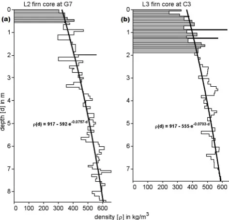
A previously identified dust layer (Dunbar et al., 2009) originating from a severe storm (with maximum southerly wind speeds exceeding 55 m s−1)that occurred on 16 May 2004 (Xiao et al., 2008) served as a reference point for dat-ing. In 2008, we found the dust layer at a depth of 2.93 m in a snow pit near stake C3 (not shown) at L2. Using the dust layer for dating, we calculate an average annual accumula-tion of 251 kg m−2a−1. In 2009, we were unable to clearly identify the dust layer in a snow pit. However, a firn core was drilled one metre east of the stake G7, to a depth of 8.46 m. Approximately at the depth at which we expected to find the dust layer, the core contained an unusually coarse grained low-density layer (starting at 3.42 m). As we found a similar low-density layer right below the dust layer in the previous year, we believe this could be a depth hoar layer that formed either as surface hoar prior to the storm or un-derneath the wind crust afterwards. Considering this as a marker for the storm in May 2004 gives an accumulation rate of 245 kg m−2a−1. Figure 5a shows the density profile of the firn core and some of the snow pit data from 2009.
At L3, no particularly distinct features could be found in a two metre snow pit in either year (not shown). Slight changes
Fig. 5. Snow density profiles in 2009 from snow pits (grey shaded
area) and firn cores at sites (a) L2 and (b) L3. In both cases, the snow pit was logged according to visually identified stratigraphy, while the core was largely logged in 10 cm intervals.
in snow grain size and hardness at about one metre depth are indicative of the previous year’s summer layer, but it was not possible to determine this with any certainty. Generally, the snow at L3 was found to be very homogeneous, with a slightly higher average density than at L2. In 2009, we drilled a firn core down to about 7.5 m near stake C3 at L3. The resulting density profile is shown in Fig. 5b. At 5.3 m depth we were able to identify a dust layer similar to that found at L2 in the previous year. Assuming that this is also associated with the May 2004 storm yields an average ac-cumulation of 437 kg m−2a−1. This value is considerably higher than the one measured by the stake farm and could ei-ther indicate an error in the dating of the dust layer, or a high inter-annual variability in snow accumulation in this area.
The firn core data can be used to determine a depth-density relationship for the two sites, as a reference for converting the vertical scale of the radargrams to depth. Following Alley et al. (1982), we determine an empirical depth(d)-density(ρ) relationship for both sites by fitting an exponential model of the form ρ(d)=ρi−a·e−c·d to the firn core data, where
Table 1. Summary of accumulation measurements at L2 (77◦450S, 167◦170E) and L3 (77◦400S, 167◦110E). Error terms represent geophys-ical variability rather than measurement error.
Site observation period years accumulation kg m−2a−1 measurement technique L2 – 81 stakes 13.11.08 – 12.11.09 1 224±21 stake reading
L2 – at stake C3 May 2004 – November 2008 4.5 251 snow pit/dust layer L2 – at stake G7 May 2004 – November 2009 5.5 245 firn core/dust layer L2 May 2004 – November 2008 4.5 269±9 GPR/dust layer
L3 – 24 stakes 18.11.08 – 9.11.09 0.97 304±83 stake reading L3 – at stake C3 May 2004 – November 2009 5.5 437 firn core/dust layer L3 May 2004 – November 2009 5.5 404±22 GPR/dust layer
14 km transect May 2004 – November 2008 4.5 270 to 165 GPR/dust layer
some densification. Therefore, the top 1.9 m of the firn core were replaced by snow pit data when determining the depth-density relationship. The resultant equations for L2 and L3 are shown in Fig. 5a and b, respectively. As the radar pro-files extend below the maximum depth of the firn cores, we also use these equations to extrapolate the density to greater depths in the following analysis. Integrating these empiri-cal relationships allows the estimation of the total snow mass to a certain depth, which can then be used to determine the mean column density, and therefore the TWT, to this depth. 4.2 Accumulation estimates from GPR measurements
The snow pit logged at L2 in 2008 is approximately located at the centre of Fig. 3c. The yellow arrow corresponds to the dust layer depth and coincides with a horizon which is more undulating than other horizons in its vicinity. The particu-larly strong roughness might be related to buried sastrugis caused by the storm event in May 2004 (Steinhoff et al., 2008; Dunbar et al., 2009). Figure 6a and b show processed radargrams from line E4 to E6 at L2, recorded in 2008 and 2009, respectively. The more undulating horizon, as well as several other reflections, are observed throughout the entire survey grid in both years (not shown). The result of tracking the dust layer horizon and eight other distinct reflections in the radar lines in Fig. 6a and b, is shown in Fig. 6c and d, respectively. The tracked reflection horizons are numbered with roman numerals from top to bottom for easier referenc-ing. The vertical scale in Fig. 6d is shifted by 4.7 ns to align the first horizon (I) in both years to facilitate comparison. The yellow line (II) in Fig. 6c is the reflection we associate with the dust horizon. Comparing its path with the neigh-bouring horizons further illustrates that it is unusually vari-able; its standard deviation from the linear trend is 0.65 ns, as opposed to 0.30 ns, 0.44 ns, and 0.34 ns for the red (I), purple (III), and black (IV) horizons, respectively.
Assuming that the undulating horizon is related to the storm-event, we can calculate the accumulation over the whole grid since May 2004. Tracking this reflection along
Fig. 6. Processed radargrams from stake E4 to E6 at site L2, recorded in (a) 2008 and (b) 2009. Nine tracked reflection hori-zons (I–IX) are shown for (c) 2008 and (d) 2009. The vertical scale in (d) is shifted up by 4.7 ns, aligning horizon I.
Fig. 7. Accumulation maps for (a) L2 and (b) L3, based on the
reflection horizon associated with the dust layer tracked along each line. A four metre interpolation grid resolution is used in both cases.
measurement error. The latter is estimated by assuming that the actual depth of the tracked layer is 16 cm (half of the theoretical resolution) above or below the measured value, giving an error of±14 kg m−2a−1. Figure 7a illustrates the variability in this reflection’s depth over the L2 area. While there is no particularly distinct pattern, it appears that accu-mulation is slightly higher in the north-east part of the grid.
Figure 8 displays a radargram of the C-line at L3 from 2009. The location of the firn core is indicated by the red box. Using the dust layer depth (5.3 m) and the densities from the firn core at stake C3, the expected TWT to the dust layer is calculated to be 49 ns (yellow arrow in Fig. 8). Com-paring this with the radargram shows that there is a clear re-flection horizon at approximately this TWT (tracked in yel-low in Fig. 8). Analogous to the approach at L2, we con-sider this as a marker for the May 2004 dust storm. Accord-ingly, the average accumulation over this site is calculated to be 404±22 kg m−2a−1. In this case the measurement error due to the resolution of the system is approximately
±13 kg m−2a−1.
The internal horizons in Fig. 8 are noticeably deeper in the middle of the profile, indicating more accumulation at the centre of the grid than at the edges. This inhomogeneity is probably related to local topography since L3 is situated on sloping terrain. The elevation difference between the lowest (I1) and the highest point (A9) is almost 20 m, with A9 lo-cated on a local crest and the terrain sloping down towards the north-west. The dip in the observed reflection horizons is on the leeward side of this crest where more drift snow accumulates. Hence, the accumulation rate calculated above needs to be considered as a large scale average for the whole area, rather than an accurate estimate at any particular loca-tion. The interpolated accumulation grid for L3 (Fig. 7b), calculated from the tracked dust layer reflection, illustrates the overall pattern. The central dip in the terrain clearly cap-tures more snow than the surrounding areas.
The decreasing trend in the depth of the dust horizon from north to south observed at L2 (Fig. 7a) can be followed south along a GPR transect (Fig. 9) that was recorded as an ex-tension of the line going from I1 to A1. Along this profile,
Fig. 8. Processed radargram from C1 to C9 at site L3 (2009). The
red box marks the approximate location of the firn core; the yellow arrow indicates the expected TWT to the dust layer.
the internal horizons gradually migrate upwards (not shown). After about 14 km, the horizon we associate with the dust layer becomes too indistinct to be reliably identified. At this point, the dust layer reflection is found at a depth of about 1.9 m, which is equivalent to a reduced average accumulation of approximately 165 kg m−2a−1(see Fig. 9). This has to be considered a crude estimate, since it assumes the same aver-age snow density between the surface and the dust layer as at L2. A qualitatively similar trend was previously reported by both Heine (1967) and the McMurdo Ice Shelf Project (McCrae, 1984).
Unfortunately, we were unable to reliably date other layers within the snow pit or firn core profiles and associate them with discrete reflections in the radargram. However, due to the high precision of the system, the vertical separation of other apparent horizons can be used to estimate compaction, which is the focus of the next section.
4.3 Snow compaction
Fig. 9. Accumulation along a transect from L2 to L1, estimated by
tracking the dust layer reflection for 14 km.
data, allows us to estimate the compaction of the snow in the intervening time period.
Not all horizons in Fig. 6c and d are suitable for com-paction calculations because the high variability of the un-dulating horizon, for example, does not allow it to be tracked reliably enough to be confident that the same horizon was se-lected in both years. Similarly, the relatively strong double-horizon visible between 41 ns and 46 ns in 2008 (Fig. 6a) and between 45 ns and 49 ns in 2009 (Fig. 6b) may be easy to recognise visually, but the noise between both horizons makes them unreliable for automated tracking. In order to establish which of the reflections are likely to be reliably tracked in both years, we calculate the correlation between the TWT profile of each horizon in 2008 and its counter-part in 2009. Additionally, we calculate the distance between pairs of horizons in terms of TWT for each year and the cor-relation of these relative TWT profiles. Only those horizons that show a correlation greater than 0.5 in all cases are used for compaction calculations. To ensure accuracy, we also re-quire a minimum average TWT difference between horizons of 10 ns, corresponding to approximately 1 m vertical sepa-ration.
Fig. 10. Snow compaction along the line from stake E1 to E9 at
L2, calculated from the changes in the average separations between some of the horizons shown in Fig. 6c and d. Horizontal error bars are a combination of the relative accuracy of the radar system and spatial variability of the horizons along the line.
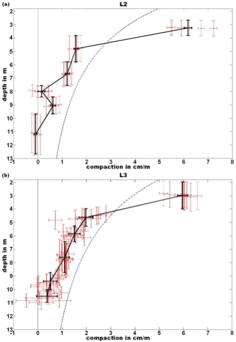
For example, the average separation of horizon III and horizon IV in 2008 is 18.7 ns (Fig. 6c), but only 18.4 ns in 2009 (Fig. 6d). This means that the snow between these two horizons was compressed by about 1.6 % during the inter-vening time period, assuming a constant wave speed. Using the density information from the firn core, this translates into a compaction of about 1.6 cm m−1. The same calculations for five other horizon pairs result in the compaction diagram shown in Fig. 10. Clearly, the compaction decreases with depth. The horizontal error bars are a combination of the standard errors of the respective horizons’ depths along the whole line (spatial variability) and the relative accuracy of the system. The vertical scale in Fig. 10 relates to the depth of the horizons in 2008, i.e. before the compaction has oc-curred. Since the time between the acquisition of the GPR datasets was nearly one year (355 days), the values in Fig. 10 can be considered estimates of annual compaction rates.
in 2008 by approximately 1 % and an increase in the com-paction rates of about 0.5 cm m−1.
The apparent expansion observed below 10 m in Fig. 10 probably indicates the error in our measurements, and the actual amount of compaction over a one year time period at this depth is too small to be measured with our system. Fur-thermore, below 8.4 m the conversion from TWT to depth is based solely on an extrapolation of the exponential fit to the density data from the firn core, causing additional uncertain-ties in the calculations.
The same calculations were performed for five more lines at L2 (A2–I2, A5–I5, A7–I7, B1–B9, and H1–H9) and are summarised in Fig. 11a. The vertical error bars indicate the average separation of the two horizons in 2008. Figure 11a shows that the variability in layer depths and compaction be-tween these six lines is small and thus tracking was not re-peated for the remaining lines. The thicker, black data points present the average compaction between each of the horizon pairs and the connecting line illustrates the decreasing trend. Figure 11b was calculated using the same methodology on seven internal horizons at L3. At this site, the variability of the compaction rates and the average depths is significantly higher. Therefore, the calculations were performed for all grid lines, except for A9–I9 due to corrupt data. The larger spread is in accordance with the observed spatial variabil-ity in the accumulation pattern and the resulting dipping of the internal horizons (see Figs. 7b and 8). Nevertheless, the mean compaction rate (black line) shows a clear trend of re-duced compaction with depth, similar to that observed at L2. Assuming constant density profiles with time (Sorge’s law) and using the measured average accumulation from the stake farms to determine the initial offsets, we can calcu-late expected compaction curves. The results are the dashed blue lines in Fig. 11a and b. In both cases the general trend matches that of the compaction measurements, but above about 4 m measured compaction rates are higher than those predicted by the model, and lower at greater depths.
5 Discussion
Table 1 summarises our results relating to accumulation. At both L2 and L3, the measurements derived from the stake farms showed significantly less accumulation than the com-bined firn core and GPR measurements. This discrepancy is probably largely due to temporal variability. If the readout of the stake depths had occurred one week later, the measure-ments at both sites would have been noticeably higher due to the occurrence of a high precipitation event from the 13 to 15 November 2009. The accumulation rates derived from the snow pit and firn core observations should therefore be con-sidered more reliable, since they cover a longer time period.
The average accumulation at L2 – a site that is rel-atively typical for coastal areas – was found to be 269±9 kg m−2a−1, which is much lower than the value re-ported by Heine (1967) at the closest station (510 kg m−2a−1
Fig. 11. Snow compaction vs. depth for (a) L2 and (b) L3.
(a) shows the compaction calculated from six lines at L2, while (b) includes all lines from L3 except one. The vertical axis
repre-sents depth before compaction has occurred. The horizontal error bars illustrate only the spatial variability along each of the lines, not measurement error. The vertical error bars show the thickness of the layers before compaction. The thick black line represents the average compaction for each horizon pair and the dashed blue line represents the expected compaction when assuming a constant density profile with time (Sorge’s law).
at station 200, about 6 km north east of our site). There is a strong accumulation gradient in this area and L2 is close to the 320 kg m−2a−1contour suggested by McCrae (1984), a value which still lies above our estimate.
Moreover, historic accumulation rates derived from stake measurements are very likely to be underestimates, as the consideration of snow compaction – as suggested by Taka-hashi and Kameda (2007) – is not reported.
The gradient in the accumulation map for L2 (Fig. 7a) is found to continue along the transect toward L1 (Fig. 9). The southernmost point up to which we were able to track the dust horizon lies relatively close to the location of a 20 m firn core analysed in Dunbar et al. (2009). They estimate an accu-mulation rate of 53±20 cm of snow per year. If we assume an average density of 600 kg m−3 for the whole length of their core, this corresponds to 318±120 kg m−2a−1. Again, our estimate from the tracked reflection lies significantly lower at 165 kg m−2a−1. However, the two points are ap-proximately 3 km apart and the conversion from TWT to depth uses the average column density down to the dust layer determined at L2, which is probably an underestimate for this location.
Only one reflection horizon could be associated with a layer in the snow stratigraphy acquired via simple glaciolog-ical tools and visual observation. Such difficulties in linking snow pit and radar observations are quite common (Harper and Bradford, 2003) and are due to the limited resolution of our density profiles (Eisen et al., 2003). Furthermore, the study sites investigated here were located in areas of low di-electric variability. The snow was dry and homogeneous and therefore contained few major dielectric contrasts, such as might be caused by occasional melt layers (e.g., Dunse et al. 2008). Alley (1988) and Arcone et al. (2004) suggest that a combination of thin layers and depth hoar are likely sources for GPR reflections in dry snow. While we did not observe many distinct hoar layers in the snow pit and core data, some may have been overlooked due to the coarseness of the recorded density profile. Accurate identification of the origin of the radar reflections would require high-resolution data from e.g. dielectric profiling, as suggested by Eisen et al. (2004) and Hawley et al. (2008).
The locations of the various horizons at the crossover points of the grid are consistent between perpendicular pro-files. In most cases, the same reflection tracked along differ-ent profiles can be found within two time samples (2×0.1 ns which corresponds to 4 cm) at the point of intersection. The concurrence of the horizon depths is equally high for all re-flections at both L2 and L3, showing that the precision of the processed radar data is higher than the theoretical resolution might suggest. This high precision allowed us to estimate snow compaction with depth from changes in the separations of internal horizons from one year to the next.
At both L2 and L3, the average compaction measured be-tween 2 and 13 m depth over a one year time period ranges from 0 cm m−1to 7 cm m−1. The sudden drop in compaction observed below about 4 m at both sites (see Fig. 11) could be related to a change in the compaction mechanism. Fresh snow largely compacts via settling, but above a density of 550 kg m−3sintering is usually considered to become
dom-inant (Maeno, 1982; Van den Broeke, 2008). According to the density profiles in Fig. 5, the 550 kg m−3level lies around 6 m depth at both sites, which compares well with the model estimate by Van den Broeke (2008), who gives a range of 5 to 8 m depth for the 550 kg m−3level in this area. However, the depth at which we observe a change in compaction rate (4 m) is more shallow than this theoretical threshold density. A re-cent study by H¨orhold et al. (2011) suggests that the “classic” picture of snow compaction is too simple, but better resolved density measurements would be required to explain the ori-gin of the observed step in compaction rate. Similarly, the origin of the dip in compaction rate between 7.5 m and 8.5 m at L2 (Fig. 11a) could be a result of above average snow den-sity at this depth, possibly related to one or two particularly warm summers, but we do not have sufficient data to test whether this is a measurement error or a subsurface feature.
High resolution measurements of densification rates to di-rectly compare with our results are sparse. As we cannot identify the 2008 surface in the radargrams from 2009, it is not possible to calculate the total compaction of the whole snow column. However, total compaction between 5 m and 10 m depth can be estimated from Fig. 11 and compared to the measurements from Arthern et al. (2010). Summing up the average compaction (black lines in Fig. 11a and b) be-tween 5 m and 10 m, gives a total compaction of approxi-mately 4.3 cm at L2 (assuming zero compaction for the deep-est 30 cm, where the results are negative) and 5.5 cm at L3, over a time period of 355 days. Using the daily rates given in Table 3 of Arthern et al. (2010) to calculate the total com-paction over the same time span and depth range gives 5.7 cm for their “Berkner Island” site, the only site at which their strainmeters worked throughout the whole trial time. While our results qualitatively agree with the “Berkner Island” data, the other sites detailed in Arthern et al. (2010) show consid-erably higher compaction rates. As mentioned above, one reason for this could be that we do not take into account the change in snow density due to compaction and its effect on the velocity of the radar signal, since this would require ad-ditional density data for 2008. Ultimately, the discrepancies between Arthern et al. (2010) and our results could also be due to a difference in climatic conditions, since most of their sites are located in regions with lower mean annual temper-ature, lower latitude, higher elevation and higher annual ac-cumulation. Therefore, considerable differences in the com-paction behaviour of the snow could be expected.
6 Summary and conclusion
associated with density variations. The processing also fa-cilitates recognition of the same horizons in follow-up sur-veys. Our methodology also has the potential to work suc-cessfully for recordings in areas that are subject to sporadic melt events, although one should keep in mind that an essen-tial assumption of the deconvolution is that there is no – or only very little – frequency dependent absorption and disper-sion in the medium.
Using the thusly processed radargrams we extrapolated point measurements of average accumulation from a snow pit at site L2 (251 kg m−2a−1) and a firn core at site L3 (437 kg m−2a−1), to a larger area by identifying a dateable dust layer horizon in the radargram. From the GPR data the extrapolated average accumulation over the 800 m×800 m site on the ice shelf in Windless Bight (L2) was found to be 269±9 kg m−2a−1. The 400 m×400 m grid on Ross Island (L3) showed higher variability in the internal horizons with an overall average accumulation of 404±22 kg m−2a−1. Stake farm readings at both sites, maintained over approx-imately a one year time period, measured an accumulation of 224±21 kg m−2a−1 at L2 and 304±83 kg m−2a−1 at L3. The discrepancy between these values and the combined firn core and GPR measurements was probably caused by the short time period spanned by the stake observations and the high temporal variability of precipitation events. Ad-ditionally, we measured a decreasing accumulation trend along a 14 km long GPR transect heading south from L2. At the southernmost point, the accumulation was about 165 kg m−2a−1.
By comparing vertical separations of internal reflection horizons from one year to the next, we were able to estimate compaction rates from GPR measurements down to 13 m depth. This technique might have implications for the val-idation of the CryoSat-2 satellite altimeter which measures the surface height of ice sheets and shelves, in order to mon-itor the polar mass balance.
Our results show that internal reflectors found in GPR data, combined with density information, can be used for es-timating compaction rates of dry snow. However, eses-timating densification in percolation areas is probably much more dif-ficult due to the more complex snow morphology (Parry et al., 2007). Frequent repetition of GPR measurements over a longer time period, combined with high resolution dielec-tric profiling of firn cores, could be used to establish a more detailed representation of time-dependent firn densification for the validation of current firn densification models. The suggested method is applicable over large areas in an effi-cient and non-invasive manner and is complementary to point measurements of snow compaction at a higher temporal res-olution, such as those performed by Arthern et al. (2010) and Heilig et al. (2010). Using a higher frequency system, it might also be possible to improve the vertical resolution of snow compaction data from GPR measurements.
Acknowledgements. The authors would like to thank Steven Arcone and Olaf Eisen for their thorough reviews and suggestions for the improvement of the manuscript. This work was supported by Antarctica New Zealand under the field event K053 “Cryosphere Remote Sensing” and by scholarships from the Christchurch City Council and the University of Canterbury for Nikolai Kruetzmann. The participation of Mette Riger-Kusk in the field work in 2008 is greatly acknowledged. The measurements were conducted within the ESA CryoSat-2 calibration and validation activities for project AOCRY2CAL-4512.
Edited by: M. Van den Broeke
References
Alley, R. B.: Concerning the deposition and diagenesis of strata in polar firn, J. Glaciol., 34(118), 283–290, 1988.
Alley, R. B., Bolzan, J. F., and Whillans, I. M.: Polar firn densifica-tion and grain growth, Ann. Glaciol., 3, 7–11, 1982.
Arcone, S. A., Lawson, D., and Delaney, A.: Short-pulse wavelet recovery and resolution of dielectric contrasts within englacial and basal ice of Matanuska Glacier, Alaska, U.S.A., J. Glaciol., 41, 68–86, 1995.
Arcone, S. A., Spikes, V. B., Hamilton, G. S., and Mayewski, P. A.: Stratigraphic continuity in 400 MHz short-pulse radar profiles of firn in West Antarctica, Ann. Glaciol., 39, 195–200, 2004. Arcone, S. A., Spikes, V. B., and Hamilton, G. S.: Stratigraphic
variation in polar firn caused by differential accumulation and ice flow: Interpretation of a 400-MHz short-pulse radar profile from West Antarctica, J. Glaciol., 51(7), 407–422, 2005. Arthern, R. J. and Wingham, D. J.: The natural fluctuations of firn
densification and their effect on the geodetic determination of ice sheet mass balance, Climatic Change, 40(4), 605–624., 1998. Arthern, R. J., Vaughan, D. G., Rankin, A. M., Mulvaney, R., and
Thomas, E. R.: In situ measurements of Antarctic snow com-paction compared with predictions of models, J. Geophys. Res., 115, F03011, doi:10.1029/2009JF001306, 2010.
Bader, H.: Sorge’s law of densification of snow on high polar glaciers, J. Glaciol., 2(15), 319–323, 1954.
Bentley, C. R., Clough, J. W., Jezek, K. C., and Shabtaie, S.: Ice-thickness patterns and the dynamics of the Ross Ice Shelf, Antarctica, J. Glaciol., 24(90), 287–294, 1979.
Belina, F. A., Dafflon, B., Tronicke, J., and Holliger, K.: Enhancing the vertical resolution of surface georadar data, J. Appl. Geo-phys., 68, 26–35, doi:10.1016/j.jappgeo.2008.08.011, 2009. Bogorodsky, V. V., Bentley, C. R., and Gudmandsen, P. E.:
Ra-dioglaciology, D. Reidel Publishing Company, Norwell, Mas-sachusetts, ISBN 90-277-1893-9, 1985.
Bracewell, R. N.: Fourier analysis and imaging, Kluwer Aca-demic/Plenum Publishers, New York, New York, ISBN 0-306-48187-1, 2003.
Davis, C. H. and Ferguson, A. C.: Elevation Change of the Antarc-tic Ice Sheet, 1995–2000, from ERS-2 Satellite Radar Altimetry, IEEE Trans. Geosci. Remote Sens., 42(11), 2437–2445, 2004. Davis, C. H., Li, Y., McConnell, J. R., Frey, M. M., and Hanna, E.:
Drinkwater, M. R., Long, D. G., and Bingham, A. W.: Greenland snow accumulation estimates from satellite radar scatterometer data, J. Geophys. Res., 106(D24), 33935–33950, 2001. Dunbar, G. B., Bertler, N. A. N., and McKay, R. M.:
Sed-iment flux through the McMurdo Ice Shelf in Windless Bight, Antarctica, Global and Planetary Change, 69, 87–93, doi:10.1016/j.gloplacha.2009.05.007, 2009.
Dunse, T., Eisen, O., Helm, V., Rack, W., Steinhage, D., and Parry, V.: Characteristics and small-scale variability of GPR signals and their relation to snow accumulation in Greenland’s percolation zone, J. Glaciol., 54(185), 333–342, 2008.
Eisen, O., Wilhelms, F., Nixdorf, U., and Miller, H.: Reveal-ing the nature of radar reflections in ice: DEP-based FDTD forward modeling, Geophys. Res. Lett., 30(5), 1218–1221, doi:10.1029/2002GL016403, 2003.
Eisen, O., Nixdorf, U., Wilhelms, F., and Miller, H.: Age estimates of isochronous reflection horizons by combining ice core, survey, and synthetic radar data, J. Geophys. Res.-Sol. Ea., 109, B04106, doi:10.1029/2003JB002858, 2004.
Eisen, O., Frezzotti, M., Genthon, C., Isaksson, E., Magand, O., Van den Broeke, M. R., Dixon, D. A., Ekaykin, A., Holm-lund, P., Kameda, T., Karlo, L., Kaspari, S., Lipenkov, V. Y., Oerter, H., Takahashi, S., and Vaughan, D. G.: Ground-based measurements of spatial and temporal variability of snow ac-cumulation in East Antarctica, Rev. Geophys., 46, RG2001, doi:10.1029/2006RG000218, 2008.
Harper, J. T. and Bradford, J. H.: Snow stratigraphy over a uni-form depositional surface: spatial variability and measurement tools, Cold Reg. Sci. Technol., 37, 289–298, doi:10.1016/S0165-232X(03)00071-5, 2003.
Hawley, R. L., Brandt, O., Morris, E. M., Kohler, J., Shepherd, A. P., and Wingham, D. J.: Techniques for measuring high-resolution firn density profiles: case study from Kongsvegen, Svalbard, J. Glaciol., 54(186), 463–468, 2008.
Heilig, A., Eisen, O., and Schneebeli, M.: Temporal observations of a seasonal snowpack using upward-looking GPR, Hydrol. Pro-cess., 24, 3133–3145, doi:10.1002/hyp.7749, 2010.
Heine, A. J.: The McMurdo Ice Shelf Antarctica – A preliminary report, New Zeal. J. Geol. Geop., 10(2), 474–478, 1967. Helm, V., Rack, W., Cullen, R., Nienow, P., Mair, D., Parry, V., and
Wingham, D. J.: Winter accumulation in the percolation zone of Greenland measured by airborne radar altimeter, Geophys. Res. Lett., 34(6), L06501, doi:10.1029/2006GL029185, 2007. H¨orhold, M. W., Kipfstuhl, S., Wilhelms, F., Freitag, J., and
Fren-zel, A.: The densification of layered polar firn, J. Geophys. Res., 116, F01001, doi:10.1029/2009JF001630, 2011.
Irving, J. D. and Knight, R. J.: Removal of wavelet dispersion from ground-penetrating radar data, Geophysics, 68(3), 960– 970, doi:10.1190/1.1581068, 2003.
Kovacs, A., Gow, A. J., and Morey, R. M.: The in-situ dielectric constant of polar firn revisited, Cold Reg. Sci. Technol., 23, 245– 256, 1995.
Maeno, N.: Densification rates of snow at polar glaciers, Memoirs of the National Institute of Polar Research, Special Issue, 24, 48– 61, 1982.
McCrae, I. R.: A summary of glaciological measurements made between 1960 and 1984 on the McMurdo ice shelf, Antarctica: a report submitted to the Antarctic Division of D.S.I.R., Auck-land, Dept. of Theoretical and Applied Mechanics: University of
Auckland, 1984.
Nguyen, A. T. and Herring, T. A.: Analysis of ICESat data using Kalman filter and kriging to study height changes in East Antarc-tica, Geophys. Res. Lett., 32, L23S03, Memoirs of the National Institute of Polar Researchdoi:10.1029/2005GL024272, 2005. Parry, V., Nienow, P., Mair, D., Scott, J., Hubbard, B., Steffen, K.,
and Wingham, D.: Investigations of meltwater refreezing and density variations in the snowpack and firn within the percolation zone of the Greenland ice sheet, Ann. Glaciol., 46, 61–68, 2007. Rial, F. I., Henrique, L., Pereira, M., and Armesto, J.: Wave-form Analysis of UWB GPR Antennas, Sensors, 9, 1454–1470, doi:10.3390/s90301454, 2009.
Rotschky, G., Rack, W., Dierking, W., and Oerter, H.: Retrieving Snowpack Properties and Accumulation Estimates From a Com-bination of SAR and Scatterometer Measurements, IEEE Trans. Geosci. Remote Sens., 44(4), 943–956, 2006.
Sensors and Software Inc.: pulseEKKO PRO – User’s Guide, Mis-sissauga, Ontario, Canada, 2006.
Spikes, V. B., Hamilton, G. S., Arcone, S. A., Kaspari, S., and Mayewski, P. A.: Variability in Accumulation Rates from GPR Profiling on the West Antarctic Plateau, Ann. Glaciol., 39, 238– 244, 2004.
Steinhoff, D. F., Bromwich, D. H., Lambertson, M., Knuth, S. L., Lazzara, M. A.: A Dynamical Investigation of the May 2004 McMurdo Antarctica Severe Wind Event Using AMPS, Monthly Weather Review, 136, 7–26, doi:10.1175/2007MWR1999.1, 2008.
Taner, M. T., Koehler, F., and Sheriff, R. E.: Complex seismic trace analysis, Geophysics, 44(6), 1041–1063, 1979.
Takahashi, S. and Kameda, T.: Snow density for measuring surface mass balance using the stake method, J. Glaciol., 53(183), 677– 680, 2007.
Turner, G.: Subsurface radar propagation deconvolution, Geo-physics, 59(2), 215–223, 1994.
Ulrych, T. J.: The whiteness hypothesis: Reflectivity, inversion, chaos, and Enders, Geophysics, 64, 1512–1523, 1999.
Van den Broeke, M.: Depth and Density of the Antarctic Firn Layer, Arct. Antarct. Alp. Res., 40(2), 432–438, 2008.
Walden, A. T. and Hosken, J. W. J.: An Investigation of the Spectral Properties of Primary Reflection Coefficients, Geophys. Prospect., 33, 400–435, 1985.
Wingham, D. J., Ridout, A. J., Scharroo, R., Arthern, R. J., and Shum, C. K.: Antarctic Elevation Change from 1992 to 1996, Science, 282, 456–458, 1998.
Wingham, D. J., Francis, C. R., Baker, S., Bouzinac, C., Brockley, D., Cullen, R., de Chateau-Thierry, P., Laxon, S. W., Mallow, U., Mavrocordatos, C., Phalippou, L., Ratier, G., Rey, L., Rostan, F., Viau, P., and Wallis, D. W.: CryoSat: A mission to determine the fluctuations in Earth’s land and marine ice fields, Adv. Space Res., 37, 841–871, 2006.
Yilmaz, ¨O.: Seismic Data Processing, Society of Exploration Geo-physicists, Tulsa, OK, USA, 1987.