Data assimilation using a hybrid ice flow model

www.the-cryosphere.net/5/315/2011/ doi:10.5194/tc-5-315-2011

© Author(s) 2011. CC Attribution 3.0 License.

The Cryosphere

Data assimilation using a hybrid ice flow model

D. N. Goldberg and O. V. Sergienko

Princeton University, Program in Atmosphere and Ocean Sciences, Princeton, USA Received: 26 August 2010 – Published in The Cryosphere Discuss.: 22 October 2010 Revised: 18 March 2011 – Accepted: 24 March 2011 – Published: 13 April 2011

Abstract. Hybrid models, or depth-integrated flow models that include the effect of both longitudinal stresses and verti-cal shearing, are becoming more prevalent in dynamiverti-cal ice modeling. Under a wide range of conditions they closely ap-proximate the well-known First Order stress balance, yet are of computationally lower dimension, and thus require less intensive resources. Concomitant with the development and use of these models is the need to perform inversions of ob-served data. Here, an inverse control method is extended to use a hybrid flow model as a forward model. We derive an adjoint of a hybrid model and use it for inversion of ice-stream basal traction from observed surface velocities. A novel aspect of the adjoint derivation is a retention of non-linearities in Glen’s flow law. Experiments show that in some cases, including those nonlinearities is advantageous in mimization of the cost function, yielding a more efficient in-version procedure.

1 Introduction

Direct observations of many parameters crucial to behav-ior of glaciers and ice sheets are practically impossible (e.g. history of ice-sheet-wide surface temperature and precipita-tion, ice fabric) and those that are feasible are logistically challenging and usually confined to specific locations (e.g. basal sediments, subglacial water pressure). Therefore, the application of inverse methods in glaciology continues to gain popularity. Although inversion for history of the at-mospheric temperature (MacAyeal et al., 1991; Dahl-Jensen et al., 1998), precipitation (Waddington et al., 2007), and firn thermal properties (Sergienko et al., 2008b) have been performed, inversions for the ice-stiffness parameter of ice shelves and ice-stream basal parameters are most common

Correspondence to: D. N. Goldberg

(daniel.goldberg@noaa.gov)

(e.g. MacAyeal, 1992; MacAyeal et al., 1995; Rommelaere, 1997; Vieli and Payne, 2003; Larour et al., 2005; Khazendar et al., 2007; Sergienko et al., 2008a; Joughin et al., 2009). Traditionally, these inversions are done in the integral least-square sense, i.e. a total misfit between observed and calcu-lated quantities is minimized. This approach is known as an optimal control or control method (MacAyeal, 1992, 1993). Alternative methods include a probabilistic approach (Chan-dler et al., 2006; Gudmundsson and Raymond, 2008; Ray-mond and Gudmundsson, 2009), and various iterative ap-proaches to solving the inverse problem using higher-order forward models (Maxwell et al., 2008; Arthern and Gud-mundsson, 2010).

A class of glaciological models involves a vertically-integrated stress balance that includes the effect of vertical shearing stresses, but also includes horizontal stress terms (the terms present in the SSA). For the purpose of discussion these models are referred to here as “hybrid” models since they combine two low-order approximations: the SSA and the Shallow Ice Approximation (SIA, Hutter, 1983). For ex-ample, Bueler and Brown (2009) heuristically combine the results of an SSA solution with an SIA solution, while Pol-lard and DeConto (2009), Schoof and Hindmarsh (2010), and Goldberg (2011) use depth-integrated forms of the horizontal stress terms. While these hybrid models account for all of the stress terms in the First Order balance, they have a computa-tional advantage in that the elliptic solve (the most expensive step) is not resolved in the vertical. Note that, unlike the First Order balance, these models do not allow depth variations of horizontal stresses. However, in the approximation to First Order is shown to be quite good under a wide range of con-ditions (Pattyn et al., 2008; Goldberg, 2011). Furthermore, two of these models (Bueler and Brown, 2009; Pollard and DeConto, 2009) have been used in time-dependent whole-continent simulations of Antarctica and Greenland. Clearly it is of value to be able to use the hybrid models as forward models in inversion procedures in order to find an optimal set of unknown parameters for these models. However, such an inversion has not yet been performed. Additionally, as use of these models becomes more common it will be advantageous to perform comprehensive and efficient analysis of the model sensitivities to a wide range of input parameters.

The control method developed by MacAyeal (1992) in-volves a construction of a model adjoint to the SSA equa-tions in order to find the gradients of the performance in-dex (or cost function) with respect to inverted parameters (basal sliding parameters in studies by e.g., MacAyeal, 1992; Joughin et al., 2009, and the ice stiffness parameter in stud-ies by e.g., MacAyeal et al., 1995; Larour et al., 2005). The adjoint model is a powerful tool that allows one, in a single step, to find derivatives with respect to a large number of pa-rameters at a point in solution space. However, in deriving this adjoint model, nonlinearities, such as the dependence of the Glen’s Law viscosity on strain rates, are ignored. It is not clear whether the inclusion of this dependence is advan-tageous to the performance of the method, since without it the adjoint equation is the same as the linear one solved iter-atively in the forward model.

In this paper we invert surface velocities for basal trac-tion fields using the hybrid model from Goldberg (2011) as a forward model. Both synthetic and observed surface veloci-ties are used in the inversions. The paper is organized in the following manner: in Sect. 2 the forward model is briefly in-troduced. The inversion scheme, which includes the adjoint model as a central part, is presented and discussed in Sect. 3, with the derivation and some of the lengthier expressions rel-egated to the Appendix A. Sections 4 and 5 present inver-sions of synthetic velocities, and results of an inversion using

satellite-inferred surface velocities on Pine Island Glacier are shown in Sect. 6. Special attention is paid to the effects of including the nonlinearities mentioned above in the adjoint model on the convergence of the inversion scheme.

2 Forward model

The forward model used in this study is the one described in Goldberg (2011). It can be derived from a variational formu-lation, using a modified form of the energy functional that leads to the First Order balance (Reist, 2005; Schoof, 2010). Using the First Order model results of the ISMIP-HOM ex-periments as a benchmark (Ice Sheet Model Intercomparison Project – Higher-Order Models, Pattyn et al., 2008), good agreement is shown for length scales larger than∼20 km in basal topography and for all length scales in basal traction. The equations are given here:

1

H∂x(H ν(4ux+2vy))+

1

H∂y(H ν(vx+uy))+∂z(νuz)=ρgsx, (1)

1

H∂x(H ν(vx+uy))+

1

H∂y(H ν(4vy+2ux))+∂z(νvz)=ρgsy, (2)

ν=B

2

u2_x+v2_y+uxvy+1

4(uy+vx)

2₊1

4u

2

z+ 1 4v

2

z 1₂−_nn

. (3) Hereuandvarex- andy-velocities, respectively,sis surface elevation,His thickness (s−b, whereb(x,y)is basal eleva-tion), andn represents the nonlinearity in Glen’s Law and in this study is equal to 3. The overline operator indicates vertically averaging, i.e.u= 1

H

Rs

budz, anduxindicates the

x-derivative of this quantity (and not the vertical average of ux). The surface is stress-free. When sliding is present, the

sliding law is in terms of the shear stress and velocity at the base. In this study, the sliding law is linear:

τ_b= −β2u (4)

atz=b.

Note that due to the inclusion of vertical shear, basal, sur-face, and depth-averaged velocity can all differ, in contrast to the SSA. This does not prevent a significant problem in terms of solving Eqs. (1)–(4), however. An iterative scheme can be developed by depth-integration of Eqs. (1) and (2), and writingu_z andu(z=b)in terms of the current iterates of depth-averaged velocity, basal stress and viscosity. (The surface velocity, while not needed in the iterative scheme, can be similarly diagnosed.) This yields a set of equations to be solved for the next iterate of depth-averaged velocity. The equations have the same structure as those solved in an iterative solution of the SSA balance, so an SSA code can be easily modified. For details, please see Goldberg (2011).

3 Adjoint model

view settings. The approach is essentially the same as in MacAyeal (1992), and similar to that of Arthern and Gud-mundsson (2010) – a steepest-descent method. The differ-ences are (a) the forward model and (b) the fact that nonlin-earities are accounted for in constructing an adjoint model. But the same paradigm of finding the search direction as a functional derivative that is then discretized (rather than by differentiating the discretized forward equations) is still ad-hered to. The effect of accounting for nonlinearities is ex-plored in the subsequent sections.

The cost function J=

Z



1 2|u

∗

s−us|2dA, (5)

whereus is horizontal velocity at the surface, the asterisk

superscript denotes observed quantities, andis the model domain, is minimized over all choices ofβ. The set of pos-sibleβ depends on the choice of basis forβ: for example, in MacAyeal (1993) it is Fourier modes and in MacAyeal et al. (1995) it is the finite element basis for velocity. Be-ginning with an initial guess forβ, the control method finds the gradient ofJ with respect to the degrees of freedom of β (subject to the constraint that Eqs. (1)–(4) are satisfied). A line search minimization then gives a new guess for β. A Fletcher-Reeves conjugate search algorithm is used (Press et al., 1992).

Typically when this control method is applied to glacio-logical models, an adjoint model is solved, and the result is used to find the gradient ofJ with respect to basal traction parameters (or other field that is being inverted for). The ad-vantage of using an adjoint model is that the derivative of a given observable value can be found with respect to a large array of input parameters for the computational cost of a sin-gle forward solve. This is in contrast to finding derivatives by direct finite differencing, which requires a separate for-ward solve for each input parameter. In this study the adjoint of the model described in the previous section is constructed directly from the differential equations, rather than discretiz-ing and takdiscretiz-ing the adjoint of the discretized model. The re-sult is a set of linear partial differential equations that are then solved in order to find the gradient ofJ. Note that this procedure does not assume any discretization details, and the discretization of the adjoint can be independent from that of the forward model.

We now present the adjoint model. Its derivation is lengthy and not entirely straightforward, and so it is left to the Ap-pendix A. Furthermore, the expressions involved in the joint itself are lengthy, so details are only given for the ad-joint of the flowline version of the model (i.e., flow in the x−z plane). The adjoint of the three-dimensional model, and its derivation, are very similar.

The flowline version of Eqs. (1)–(3) is

∂x(4νH ux)−τ−ρgH sx=0, (6)

τ=mβ2ub, m=

q

1+b_x2, (7)

ν=B

2(u

2

x+

1 4u

2

z)

1−n

2n _{. (8)}

Here ub=u(z=b). In our flowline inversions, periodic

boundary conditions are considered.

As in MacAyeal (1993), the cost functionJ is modified: the flowline model appears as a constraint, with lagrange multiplierλ:

J0= Z L

0

1 2(u

∗

s−us)2dx+ Z L

0

λ[∂x(4νH ux)−τ−ρgH sx]dx, (9) where[0,L]is the domain. An adjoint model is then derived that must be solved forλ:

∂x(4νH λx)−

mβ2 1+mβ2γ

H τ

λ+F{λ;u,β,x}

=(u∗_s−us) 1+

mβ2γs

H τ+mβ2γ !

+G{u∗_s−us;u,β} (10)

whereF andGare linear operators on their first arguments (λandu∗_s−us, respectively) that also depend onuandβ.γ

andγsare functions that depend on the gradients ofu:

γ=

Z s b

Z z b

u2_x+1

4u

2

z

u2_x+ 1

4nu2z

uzdz0dz,

γs=

Z s b

Z s z

u2_x+1

4u2z

u2_x+ 1

4nu2z

uzdz0dz, (11)

and F andG are given in the Appendix A. (Note that if n=1, thenγ andγs are equal toH (u−ub)andH (us−u),

respectively.) Equation (10) is solved for λ with appro-priate boundary conditions: if the boundary conditions on Eq. (6) are Dirichlet, then Eq. (10) has homogeneous Dirich-let boundaries. If Eq. (6) has periodic boundary conditions, then Eq. (10) does as well. Note that the form of the adjoint model Eq. (10) is dependent on the forward model and the form of the cost functionJ, but would be the same no matter which input parameter is being investigated. However, in this study the goal is to find the gradient ofJ0with respect toβ, which is done using the following:

δJ0=

Z L

0

−δβ 



(u∗_s−us)2_Hγs+2τ λ+K{λ;u,β}

β1+mβ2γ

H τ



, (12)

which gives the response ofJ0to a perturbation inβ. Again, K is a linear operator on λ, the specific form of which is given in the Appendix A. With a finite-dimensional repre-sentation ofβ, Eq. (12) can then be discretized to find ∂J_∂β0

i, whereβiare the degrees of freedom in such a representation,

i.e. β=X

i

whereφi form the basis of the space of possibleβ. Thusδβ

is written as δβ=X

i

φiδβi. (14)

Equation (10) is written in such a way (i) because the ex-pressions forF,G, andK are lengthy, and (ii) in order to emphasize the effect of ignoring the dependence of viscosity on strain rates, something quite often done in glaciological inversions using adjoints (MacAyeal, 1993; Vieli and Payne, 2003; Larour et al., 2005; Joughin et al., 2009). Doing so here is equivalent to neglectingF,G, andK, and addition-ally lettingn=1 in Eq. (11). The adjoint model withF and Gleft in andn6=1 will subsequently be referred to as the

complete adjoint and, withF andGignored andn=1 as the

incomplete adjoint.

It is interesting to note that in doing this, the operator given by the left hand side of Eq. (10) is the same as the forward model when the viscosity is “frozen”, as in a Picard-iterative solution (MacAyeal and Thomas, 1986). This is not a coin-cidence; when the strain-rate dependence of viscosity is ig-nored, the equation system in Goldberg (2011) is linear and self-adjoint under theL2 inner product. (This is also true

of the three-dimensional model.) Thus using the incomplete adjoint saves on development time and also ensures that the adjoint model has the same desirable properties as the for-ward model (i.e., that the matrix that is solved is symmetric and positive definite). If the matrix is solved in parallel, the domain decomposition and parallel memory allocation need not change. As discussed in Goldberg (2011), the compu-tationally expensive component of the hybrid model is the solution of a system of elliptic PDEs with the same structure as those solved for the SSA balance.

However, the adjoint model is only solved once per iter-ation of the inverse model, so it is possible that relaxing the property of self-adjointness will not carry too large a penalty. In the following sections, flowline and 2-D (plan view) inver-sions are carried out, and the effects of including such non-linearities in the adjoint model are examined. An important point to remember is that, with the same forward model and cost function, the only way in which these effects can man-ifest is in the rate of convergence of the inversion. Whether nonlinearities are included or not, the solution (or set of so-lutions) of an inversion is the same.

In this study, the forward and adjoint models are solved using one-dimensional or bilinear finite elements as in Gold-berg (2011) and GoldGold-berg et al. (2009), andφi is equal to 1

on grid celliand zero elsewhere. Still, the discussion above does not depend on specific details of the discretization.

4 Flowline inversion

A flowline version of the hybrid model was used to invert synthetic surface velocities for basal traction, assuming a lin-ear sliding law. The experiments are based on the flowline

experiments with sliding from the ISMIP-HOM intercompar-ison. The domain is periodic, and ice thickness has a constant value of 1000 m and a surface at an angle of 0.1◦_{with the}

horizontal, and the Glen’s Law constant is uniformly equal to 2.1544×105Pa (m a−1)−13_{. The velocities inverted forβ} are the surface velocities from a First Order flowline solver (that used in Goldberg, 2011) with the same thickness, sur-face slope, and Glen’s Law constant, and aβ-profile given by

β=

s

1000+1000 sin(2π x Lx

)Pa12_{(m a}−1₎− 1

2 ₍₁₅₎

where basal stress is given by

τb=β2u|z=b, (16)

andLxis the length of the domain. As shown in Goldberg

(2011), the hybrid model surface velocities agree well with First Order surface velocities in this setting. And so while these inversions are known to be ill-posed, and thus many different β-profiles could produce surface velocity profiles close to the “target” one, we still know that Eq. (15) is a valid solution to the inverse problem, or at least leads to an cost function value as small as any achieved in this study (Gold-berg, 2011). Maxwell et al. (2008) state that their method finds the solution to the inverse problem for which noisy os-cillations are minimized. And so we can judge our inver-sion results not only by the agreement of calculated and pre-scribed surface velocities, but also by the agreement of the invertedβwith Eq. (15).

For an inversion scheme, both the incomplete adjoint men-tioned in the previous section and the complete adjoint were used. In all inversions, the initial guess forβwas set to a uni-form value. 300 iterations of the inverse model were done, regardless of the final value ofJ.

Figure 1 shows the results of such an inversion with a domain length of 40 km. Inversions using both incomplete (dashed line) and complete (solid line) adjoints are shown. Values ofJversus iteration count are shown, as well as the fi-nal invertedβ2(which is compared withβ2given by Eq. 15). Comparison is made usingβ2rather thanβsince it isβ2that appears in Eq. (16). In the left column, the initial guess for β is 20 Pa12_{(m a}−1₎−

1

2 _{(uniformly), and in the right the} ini-tial guess is 40 Pa12(m a−1)−

1

2_{. With either initial guess, the} complete adjoint reaches a much smaller value ofJ than the incomplete adjoint (by several orders of magnitude) and finds a solution very close to Eq. (15), while the incomplete ad-joint finds a highly oscillatory solution. Using the complete adjoint,J decreases steadily, while with the incomplete ad-joint most of the reduction ofJis in the first few oscillations. In fact, with the initial guess of 20 Pa12_{(m a}−1₎−

1

0 50 100 150 200 250 300

102

104

106

108

iteration #

J

incomp. adj. complete adj.

0 20 40 60 80 100 120 140 160

100

102

104

106

108

iteration #

J

incomp. adj. complete adj.

(a) Cost functionJ vs. iteration count,βinit=20 (Pa a/m)

1

2 (b) Cost functionJvs. iteration count,βinit=40 (Pa a/m)

1 2

0 0.5 1 1.5 2 2.5 3 3.5 4

x 104

0 1000 2000 3000 4000 5000 6000

x (m)

β

2 (Pa m

−1

a)

incomp. adj. complete adj. "true" β2

0 0.5 1 1.5 2 2.5 3 3.5 4

x 104

0 2000 4000 6000 8000 10000 12000 14000

x (m)

β

2 (Pa m −1 a)

incomp. adj. complete adj. "true" β2

(c) Invertedβ2,βinit=20 (Pa a/m)

1

2 (d) Invertedβ2,βinit=40 (Pa a/m)

1 2

Fig. 1. Results of inversion forβ2, using the flowline model with periodic boundary conditions and uniform thickness and basal slope.

Domain length is 40 km. “Observed” surface velocities are the results of a First Order flowline model calculated using “true”βfrom (c) and

(d). Initial guess forβis set uniformly to 20 (Pa a/m)12 in the first column and to 40 (Pa a/m)12 in the second column.

found by the complete adjoint scheme is relatively insensi-tive to the initial guess forβ.

Figure 2 shows the results for a domain length of 20 km, with an initial guess for β of 20 Pa12_{(m a}−1₎−

1

2_{. Here the} contrast between the complete and incomplete adjoints are even more apparent. The complete adjoint steadily reduces J and finds a solution that is reasonably close to Eq. (15), while the incomplete adjoint barely adjustsβfrom its initial guess and does not reduceJ after the very first iteration. No other initial guess was examined for this domain length.

The ability of the adjoint models to represent derivatives, particularly derivatives of surface velocities, can be exam-ined. The calculation of such derivatives can be cast in terms of the adjoint method: using the fact that

Ji≡us(xi)=

Z L

0

usδxi(x)dx, (17)

whereδxi(x)is the Dirac delta function shifted by xi, the same approach as described above is applied to

J_i0=

Z L

0

usδxi(x)dx+ Z L

0

λ[∂x(4νH ux)−τ−ρgH sx]dx, (18) and the adjoint model is again derived, but with a different right hand side than Eq. (10). The expressions are not given here, but again it is simple to separate out the terms corre-sponding to the strain-rate dependence of viscosity.

Figure 3a shows the Jacobian of surface velocities with respect to basal traction values, calculated directly by finite differencing. (With no analytic expression for the Jacobian, this is taken as the “true” value.) Basal traction is given by Eq. (15) and there is no topography. The figure can be seen as a contour plot of ∂u(xi)

∂β(xj), where xi is along the horizon-tal axis andxj the vertical. Figure 3b shows this Jacobian

0 50 100 150 200 250 300

102

103

104

105

106

107

iteration #

J

incomp. adj. complete adj.

0.2 0.4 0.6 0.8 1 1.2 1.4 1.6 1.8

x 104

0 500 1000 1500 2000 2500

x (m)

β

2 (Pa m

−1

a)

incomp. adj. complete adj. "true" β2

(a) Cost function vs. iteration count,Lx=20 km (b) Invertedβ2,Lx=20 km

Fig. 2. Same as Fig. 1, with domain length of 20 km. Initial guess forβ2set uniformly to 20 Pa12 (m a−1)−12.

the way the gradient ofJ with respect toβ is found. Fig-ure 3c is the equivalent calculation using the incomplete ad-joint model. Quite a difference between the two can be seen, especially for the derivatives of the velocities in the “slip-pery” region with respect to the traction values in the “sticky spot”. It seems that using the incomplete adjoint model un-derestimates these sensitivities, and therefore overshoots in its guess for these traction values, leading to the oscillations seen in Figs. 1c and 2b.

It was noted in Goldberg (2011) that in the ISMIP-HOM tests of nonsliding flow over wavy topography, agreement of the hybrid model with First Order surface velocities was not as good as in the tests of sliding flow over periodic traction. Inversion for basal topography was not done in this study; however, it is fair to ask whether the presence of basal to-pography would affect the results presented in this section. A series of tests was done where there is still sliding at the base, but the basal elevation varies from the mean slope sinu-soidally with the same wavelength as the basal traction and an amplitude of 100 m (compare with 500 m in the ISMIP-HOM experiments). The results were very similar to those in Fig. 1, and not shown.

5 Plan view inversion – synthetic data

The ISMIP-HOM intercomparison also includes a set of three dimensional experiments, one of which involves sliding over varying basal traction in a doubly periodic domain. Sur-face velocities from this experiment were inverted for basal traction, and the results are shown here. Both the complete and incomplete adjoints were used. The forms and deriva-tions of these models are very lengthy and not shown, but they are simple extensions of the flowline adjoint models dis-cussed in the Appendix A. Since a three-dimensional First Order solver was not used in this study, a mean was taken

over the publicly available results from the intercomparison that solved the First Order balance (http://homepages.ulb.ac. be/∼_{fpattyn/ismip/tc-2-95-2008-supplement.zip).}

In this experiment the Glen’s Law constant and the (uni-form) thicknessH had the same values as in the flowline experiments. While not directly used, the basal traction spec-ified for the ISMIP-HOM experiment is

βih=

s

1000+1000sin(2π x Lx

)sin(2πy Ly

)Pa12_{(m a}−1₎− 1 2_,(19)

whereLx andLy are the x- and y-dimensions of the

do-main. As discussed before, this may not necessarily be the only possible solution of the inversion, but it is useful for comparison.

In the plan view inversions, it was found that when the initial guess forβ was constant, the residualJ did not de-crease by much even after a large number of iterations, using either the complete or incomplete adjoint models (see Dis-cussion and conclusions). Instead, two different spatially-varying initial guesses forβwere considered:

β1=10+20e

−(x−Lx )2−(y−Ly )2 (1₆Lx )2

!

Pa12_{(m a}−1₎− 1

2_{, (20)}

β2=

s

sin(3π x Lx

)Pa12_{(m a}−1₎− 1

2_{. (21)}

Note thatβ1is a Gaussian “bump” in the middle of the

do-main, whileβ2is sinusoidal inx(but not iny), but its peaks

and troughs do not correspond to those of Eq. (19).

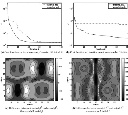
The results of the inversion are shown in Fig. 4, forLx

andLy equal to 40 km. The left column corresponds to

us-ingβ1as an initial guess, and the right toβ2. The top row

velocity position (m)

β

position (m)

0.5 1 1.5 2 2.5 3 3.5 x 104 0.5

1 1.5 2 2.5 3 3.5

x 104

−0.3 −0.25 −0.2 −0.15 −0.1 −0.05

velocity position (m)

β

position (m)

0.5 1 1.5 2 2.5 3 3.5 x 104 0.5

1 1.5 2 2.5 3 3.5

x 104

−0.3 −0.25 −0.2 −0.15 −0.1 −0.05

velocity position (m)

β

position (m)

0.5 1 1.5 2 2.5 3 3.5 x 104 0.5

1 1.5 2 2.5 3 3.5

x 104

−0.3 −0.25 −0.2 −0.15 −0.1 −0.05

(a) Calculation with finite differences (b) Calculation with complete adjoint (c) Calculation with incomplete adjoint

Fig. 3. Jacobian of surface velocities with respect to basal traction values. ∂u(xi)

∂β(xj)is plotted, wherexi is along the horizontal axis andxjthe vertical.

0 20 40 60 80 100

106

108

1010

1012

iteration #

J

incomp. adj. complete adj.

0 20 40 60 80 100

106

108

1010

1012

iteration #

J

incomp. adj. complete adj.

(a) Cost function vs. iteration count, Gaussian hill initialβ (b) Cost function vs. iteration count, wavenumber 3 initialβ

x (km)

y (km)

5 10 15 20 25 30 35

5 10 15 20 25 30 35

−100 −50 0 50 100 150

x (km)

y (km)

5 10 15 20 25 30 35

5 10 15 20 25 30 35

−800 −600 −400 −200 0 200 400 600 800 1000

(c) Difference between invertedβ2and actualβ2, (d) Difference between invertedβ2and actualβ2,

Gaussian hill initialβ wavenumber 3 initialβ

Fig. 4. Results of inversion in doubly-periodic domain,Lx=40 km. “Observed” surface velocities are from results of ISMIP-HOM 3-D

Jafter 100 iterations with either the complete or incomplete adjoint. However,J converges more quickly using the com-plete adjoint. Withβ2as an initial guess, there is almost no

decrease inJ using the incomplete adjoint, while using the complete adjoint achieves a decrease inJ comparable with theβ1case.

The bottom row of Fig. 4 showsβ2−β_ih2, whereβ here is found using the complete adjoint. In the case whereβ1is the

initial guess, the final invertedβ using the complete and in-complete adjoints are very similar, though this is not true for theβ2case. In theβ1case, traction in the “slippery regions”

(the top left and bottom right) is slightly overestimated and is slightly underestimated at the centers of the “sticky spots” (bottom left and top right), but overall the agreement is good. There is no remnant of the initial guess seen in the misfit. On the other hand, in theβ2case the misfit is overwhelmed by

a transverse strip at x=Lx

2, where β2 should be equal to

∼1000 Pa (m a−1)−1but is instead close to zero. This is in-deed a remnant of the initial guess, sinceβ2is zero along this

line. Since horizontal stresses tend to damp out small scales in basal traction this does not have a large effect on the cost functionJ, but it demonstrates some dependence on initial guess.

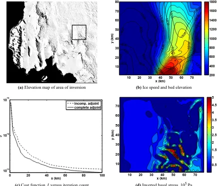
6 Plan view inversion – real data

In addition to synthetic surface velocities, inversions were done using InSAR- and speckle tracking derived surface ve-locities (Joughin, 2002) and 5 km gridded ice thickness and bed elevation data from the Airborne Geophysical Survey of the Amundsen Sea Embayment, Antarctica (AGASEA) conducted during the 2004–2005 austral summer (Vaughan et al., 2006) (these data are available from http://nsidc.org/ data/nsidc-0292.html). An 80×80 km region containing the grounded portion of Pine Island Glacier (PIG) was selected. (This region contains the areas referred to as the “ice plain”, the “steepening”, and the “trunk” by Payne et al., 2004.) The object of this exercise was not to ask specific glaciolog-ical questions; many studies have used established inversion methods to investigate basal properties of PIG (e.g. Payne et al., 2004; Joughin et al., 2009; Morlighem et al., 2010a). Rather, the purpose is to assess the convergence properties of the hybrid model inversion scheme with “real” data.

The boundary conditions of this inversion differ from the previous plan view inversions in that they are not periodic. The depth-averaged velocities at the boundary of the domain are constrained to be the interpolated InSAR surface veloci-ties. (As discussed in Goldberg (2011), lateral boundary con-ditions can only influence the solution through their depth average.)

Figure 5c shows the convergence behavior of the incom-plete and comincom-plete adjoints, with an initial, uniform guess for βof 10 Pa12_{(m a}−1₎−12_{. Basal stress}|τ|corresponding to the complete adjoint is shown in Fig. 5d. (We show basal stress

rather than β2, since in this experiment velocities are not derived synthetically using an analytical expression forβ.) Additionally, the relative importance of vertical shear in the corresponding forward model solution is shown by Fig. 5e, in which

|us−ub|

|us|

(22) is plotted. For much of the region speed due to vertical shear is less than 20% of the the surface speed, but there are areas (ones that coincide with high basal traction) where vertical shear accounts for up to 80% of the surface speed. Such ar-eas could not be resolved with the SSA model as the forward model, due to its assumption of no vertical shear. The cor-responding fields from the inversion with the incomplete ad-joint are very similar both in magnitude and spatial pattern, and are not shown.

The convergence behavior shown in Fig. 5c differs from that seen in the experiments using synthetic observations. First, the cost functionJis not lowered by as many orders of magnitude. This is expected, though, since the synthetic sur-face velocities were generated using a flow model to which the forward model is a very close approximant. Second, the difference in convergence rate between the complete and in-complete adjoints is not as dramatic. Inversion with both choices finds similar solutions, and at comparable iteration counts, the cost function in the incomplete adjoint inversion is at most twice that of the complete adjoint inversion. Still, the fact that this is achieved early in the inversion (between 10 and 20 iterations) shows that the complete adjoint could still have some utility.

In further contrast to the prior experiments, sensitivity to the initial guess of β was observed with the complete ad-joint. When the initial guess for β was very high (30– 40 Pa12(m a−1)−

1

2), no convergence was observed for either choice of adjoint. The observed behavior of J was simi-lar to that seen for the incomplete adjoint in the synthetic data experiments: almost no decrease in J was observed. Despite the results of the synthetic-observation experiments, this demonstrates a strong sensitivity of the inversion process to the initial guess of the inverted parameters. The techni-cal aspects of this issue are beyond the scope of the present study, and are the subject of further investigations.

An important consideration is whether the result of such an inversion is appropriate for the forward model. In Gold-berg (2011) solutions of the hybrid model were compared with First Order solutions. It was found that the models were in good agreement when the basal slope was smaller than

200 400

400

600 600

800

800

800

100 0 1000 1000

1000 1200

1200

120 0

1200

12 00 120

0 1400

1400

1400

1400 1400 1600

1600 1600

160 0 1800

1800 180

0

x (km)

y (km)

10 20 30 40 50 60 70

10 20 30 40 50 60 70 80

200 400 600 800 1000 1200 1400 1600 1800

(a) Elevation map of area of inversion (b) Ice speed and bed elevation

0 20 40 60 80 100

1013

1014

1015

x (km)

J

incomp. adjoint complete adjoint

x (km)

y (km)

10 20 30 40 50 60 70

10 20 30 40 50 60 70

0.5 1 1.5 2 2.5 3 3.5 4 4.5 5

(c) Cost functionJversus iteration count (d) Inverted basal stress, 105Pa

x (km)

y (km)

10 20 30 40 50 60 70

10 20 30 40 50 60 70

0.1 0.2 0.3 0.4 0.5 0.6 0.7 0.8

(e) Importance of vertical shear

surface velocities of Pine Island and Thwaites Glaciers us-ing an SSA forward model, note that the forward model bal-ance is not strictly applicable in strong-bedded regions. It is possible that inversions with a hybrid model can give more complete results without using a three-dimensional forward model.

However, it should be noted that the above statements may not apply for regions where First Order approximations are violated (i.e. near the grounding line). Morlighem et al. (2010a) compared inversions of PIG and its catchment and tributary region using SSA, First Order, and Full Stokes for-ward models. Their results showed that nonhydrostatic ef-fects were of leading-order importance in the grounding zone (part of which protrudes into the bottom of our domain, be-tween∼40 and 60 km in thex-direction), where the sharply rising bed exerts a backpressure on the flow.

7 Discussion and conclusions

Including the nonlinear terms in Eqs. (10) and (12) (i.e., us-ing the complete adjoint instead of the incomplete adjoint) does not change the solution of the inversion; it can only af-fect whether the inversion scheme finds a minimum of Eq. (5) and the speed of convergence. In this sense the flowline in-versions demonstrated a clear advantage in including these terms. Use of the complete adjoint resulted in fast conver-gence toward a minimum with relative independence on ini-tial guess, which was not the case for inversions using the incomplete adjoint.

In the plan view inversions of synthetic data, the rate of convergence improved with the inclusion of nonlinear terms. However, there was no convergence when the initial guess forβ was spatially uniform, whether nonlinear terms were included or not. This is due to specifics of the model set up, namely the periodic boundary conditions. With such condi-tions and a uniformβ, the forward model solution is a ve-locity field that does not vary inx ory, and so has a small effective strain rate (entirely due to vertical shear) and a high Glen’s Law viscosity. The result is that the search direction found by the adjoint model is nearly uniform, even though the misfit(u∗_s−us)has relatively large variation. This effect

was verified by decreasing the Glen’s Law coefficientB for the first few iterations (not shown).

In the plan view versions of observational data, the im-provement of convergence rate was not as dramatic as for of synthetic data, and also the relative insensitivity of the com-plete adjoint inversion to initial guess seemed to disappear. We point out that there are several reasons why performance of the complete adjoint model does not show a dramatic im-provement over the incomplete adjoint. First, there are limi-tations of the forward model associated with small scales in surface velocity and bed heterogeneity. Second, and perhaps more important, the data sets used in the inversion – bed ele-vation, ice thickness, and surface velocities – were obtained

by different techniques during different time periods, and are incompatible (Morlighem et al., 2010b). Such data incom-patibility has a strong effect on the inversion process. By contrast, complete versus incomplete adjoint may give a fine-tuning effect which is overshadowed by stronger factors. The effects of data compatibility on the results of inversion with a hybrid model are a subject of ongoing investigation.

Still, the PIG inversion shows a small but noticeable dif-ference was seen after a relatively small number of iterations. Since inversions might involve a cutoff after a target residual has been reached rather than a fixed number of iterations, this shows that the complete adjoint may still have some utility in such inversions, provided it is not too expensive to calculate relative to the incomplete adjoint.

Using a hybrid model that accounts for vertical shear within the ice as a forward model has several advantages. Among them are possibilities to invert (or optimize) for pa-rameters over regions that cannot be described by a single zero-order approximation (SIA or SSA) but do not require treatments of Full Stokes models. Bost fast, streaming and slow, vertical shear-driven flow regimes can be considered in the same domain. The hybrid model is computationally more efficient than First Order models, and produces solu-tions of the same order of accuracy in a wide range of condi-tions appropriate to ice modeling. The derived adjoint model could be used for numerous applications: from inversion for other model parameters to model sensitivity studies. The ad-joint is derived directly from the forward model equations rather than from their discretized equivalents, so the dis-cretization of the adjont does not depend on that of the for-ward model. The use of a glacial flow model and its adjoint to invert for unknown flow parameters is not new; however, such approaches typically ignore the dependence on strain rates of the nonlinear viscosity. In this study it is seen that, for this particular forward model, including this dependence can have a measured effect on the convergence of the inver-sion scheme. The model from Goldberg (2011) was the only one considered; however, similar flow models are being de-veloped or are already being used in large-scale ice models (e.g., Pollard and DeConto, 2009; Schoof and Hindmarsh, 2010), and the results of this study may indicate that inclu-sion of this dependence may be necessary for data assimila-tion using such models.

the initial guess. It is worth investigating whether the modi-fied cost function or regularization term of Morlighem et al. (2010a) changes any of the results of our study.

Inversion of surface velocities for basal traction numbers was the only application of an adjoint model considered in this study, but there are others. Heimbach and Bugnion (2009) examined the sensitivity of the evolution of the Green-land Ice Sheet to initial conditions by deriving an adjoint model for the ice sheet model SICOPOLIS (Greve, 1997) using automatic differentiation tools. While that version of SICOPOLIS made use of the SIA balance to calculate veloc-ities, the need for a similar study involving a model that uses a higher-order stress balance was underlined in their paper. The availability of continental-scale ice sheet models that do so, such as PISM (Bueler and Brown, 2009) or that of Pollard and DeConto (2009) present the possibility for such a study. In these models, the solution of the stress balance for veloci-ties is but a single component of a timestep (the others being evolution of thickness, temperature, and in some cases basal water and isostasy); however, it is the only component that requires the iterative solution of a nonlinear elliptic equation. Solvers of such equations involve indirect matrix solvers, preconditioners, stopping conditions and indeterminate iter-ation counts. Applying automatic differentiiter-ation techniques to these solvers could result in lengthy computation in the derivation of an adjoint. Instead, it may be possible to ana-lytically derive an adjoint for the elliptic solver and integrate it with the techniques used by Heimbach and Bugnion. With such a strategy it is worth considering both complete and in-complete adjoints. The structure of the inin-complete adjoint would make it somewhat easier to develop a solver. On the other hand, it was shown in the flowline experiments that the complete adjoint can, in some cases, give a more faithful representation of derivatives. With a time-dependent model, there is potential for accumulation of errors over multiple timesteps, and using a better representation of model deriva-tives would help to control these errors.

Appendix A

Deriving the adjoint model is basically the same as is done in MacAyeal (1993), but due to the complexity added by the inclusion of vertical shear and depth integration, the steps are shown and the form is given explicitly. Only the adjoint of the flowline version of the model is shown here; the form of the three-dimensional (plan view) adjoint is derived similarly but is more lengthy.

The flowline version of the hybrid model is stated again here:

∂x(4νH ux)−τ−ρgH sx=0, (A1)

τ=mβ2ub, m=

q 1+b2

x, (A2)

ν=B

2(u 2 x+ 1 4u 2 z)

1−n

2n _{. (A3)}

Additionally, νuz=

τ (s−z)

H . (A4)

Boundary conditions onuare periodic.

As in (MacAyeal, 1993), the adjoint model is derived by taking a first-order differential of J0 from Eq. (9). While taking the first variation does not involve any mathematical complexity, the fact that the viscosity is depth-integrated in Eq. (A1) anduz andτ seem to depend on each other in a

circular fashion makes things a bit more difficult. For that reason, it is shown here how perturbations inJ0 are related to perturbations inuandβ.

Under a perturbation inu, there is a corresponding pertur-bation inν, derived from Eq. (A3):

δν=

₁₋ n 2n

_ν(2u

xδux+1₂uzδuz)

u2_x+1

4u2z

. (A5)

Hereδuzis the vertical derivative ofδu, or equivalently the

perturbation inuz, and similarly forδux. Through Eq. (A4),

the perturbation ofuzcan be related toδτ andδu:

δuz=

δτ

νH(s−z)− τ

ν2_Hδν(s−z) (A6)

=uz

τ δτ− ₁₋ n 2n uz

2uxδux+1₂uzδuz

u2_x+1

4u2z

(A7)

=uz

τ δτ−

1−n 2n

uz

2uxδux u2_x+1

4u2z

−

1−n

2n

uz

1 2uzδuz

u2_x+1 4u2z

, (A8) which is rearranged to give

δuz



1+

1−n

4n

u2_z u2_x+1

4u2z

 =   δτ τ −

21₂−_nnuxδux

u2_x+1

4u2z



uz, (A9)

or

δuz=

uz

τ

u2_x+1

4u

2

z

u2_x+ 1

4nu2z

! δτ−

21₂−_nnuxuz

u2_x+ 1

4nu2z

δux. (A10)

Since ub=u−

1 H Z s b Z z b

uzdz0dz, (A11)

and since the perturbation and integration operators com-mute, the perturbation ofubis

δub=δu−

δτ H τ Z s b Z z b

u2_x+1

4u2z

u2_x+ 1

4nu2z

uzdz0dz

+2 _1−n

2n _u

xδux

H Z s b Z z b uz

u2_x+ 1

4nu2z

dz0dz. (A12) From the sliding law Eq. (A2), the perturbation inτ is

which leads to δτ= m

3_β2

1+m3β2γ

H τ

δu+ 2τ

β(1+m3β2γ

H τ )

δβ

+

41₂−_nnm3β2ux

H+m3β2γ

τ δux Z s b Z z b 1

2uz

u2_x+ 1

4nu2z

dz0dz. (A14)

The perturbation of the surface velocity can also be stated in terms of depth-averaged perturbations. This is done using us=u+

1 H Z s b Z s z

uzdz0dz, (A15)

along with the expressions for δuz andδτ, resulting in an

expression similar to Eq. (A12).

The pieces are now all in place. It remains to proceed as in MacAyeal (1993): finding the the first variation ofJ0 with respect to a perturbationδuand setting it to zero gives Eq. (10). Then settingδu=0 and considering a perturbation δβ leads to Eq. (12). The terms in Eqs. (10) and (12) that apply only to the complete adjoint are given here:

F{λ;u,β} =

∂x      4

_1−n n

u2_xα1+

21−_nn2α2mβ2uxψ

H τ+mβ2_γ



 λx

   −  

1−n

n

uxα2mβ2

τ+mβ2γ

H



λx−

" mβ2 1+mβ2γ

H τ

# λ

+∂x





21−_nnmβ2uxψ

H+mβ2γ

τ

λ 

, (A16)

K{λ;u,β} = 2 _1−n

n

α2uxλx, (A17)

G{u∗_s−us;u,β} =

−∂x

"

(u∗_s−us)

_1−n 2n

_4mγ

sβ2uxψ

H (H τ+mβ2_{γ )}

#

, (A18)

where α1=

Z s b

ν u2_x+ 1

4nu2z

dz, α2=

Z s b

νu2_z u2_x+ 1

4nu2z

dz, (A19) ψ= Z s b Z z b 1

2uz

u2_x+ 1

4nu2z

dz0dz,

ψs=

Z s

b

Z s

z

1

2uz

u2_x+ 1

4nu2z

dz0dz. (A20)

Acknowledgements. D. Goldberg is supported by AOS/GFDL fellowship, O. Sergienko is supported by NSF grants OPP-0838811 and CMG-0934534.

Edited by: G. H. Gudmundsson

References

Arthern, R. J. and Gudmundsson, G. H.: Initialization of ice-sheet forecasts viewed as an inverse Robin problem, J. Glaciol., 56, 527–533, 2010.

Bueler, E. and Brown, J.: The shallow shelf approximation as a “sliding law” in a thermomechanically coupled ice sheet model, J. Geophys. Res.-Earth, 114, F03008, doi:10.1029/ 2008JF001179, 2009.

Chandler, D. M., Hubbard, A. L., Hubbard, B. P., and Nienow, P. W.: A Monte Carlo error analysis for basal slid-ing velocity calculations, J. Geophys. Res., 111, F04005, doi:10.1029/2006JF000476, 2006.

Dahl-Jensen, D., Mosegaard, K., Gundestrup, N., Clow, G. D., Johnsen, S. J., Hansen, A. W., and Balling, N.: Past Tempera-tures Directly from the Greenland Ice Sheet, Science, 282, 268– 271, 1998.

Glen, J. W.: The creep of polycrystalline ice, Proc. R. Soc. Lon. Ser.-A, 228, 519–538, 1955.

Goldberg, D. N.: A variationally-derived, depth-integrated approxi-mation to a higher-order glaciologial flow model, J. Glaciol., 57, 157–170, 2011.

Goldberg, D. N., Holland, D. M., and Schoof, C. G.: Grounding line movement and ice shelf buttressing in marine ice sheets, J. Geophys. Res.-Earth, 114, F04026, doi:10.1029/2008JF001227, 2009.

Greve, R.: A continuum-mechanical formulation for shallow poly-thermal ice sheets, Philos. T. R. Soc. Lond., 355, 921–974, 1997. Greve, R. and Blatter, H.: Dynamics of Ice Sheets and Glaciers,

Springer, Dordrecht, 2009.

Gudmundsson, G. H. and Raymond, M.: On the limit to resolution and information on basal properties obtainable from surface data on ice streams, The Cryosphere, 2, 167–178, doi:10.5194/tc-2-167-2008, 2008.

Heimbach, P. and Bugnion, V.: Greenland ice-sheet volume sen-sitivity to basal, surface and initial conditions derived from an adjoint model, Ann. Glaciol., 50, 67–80, 2009.

Hutter, K.: Theoretical Glaciology, Dordrecht, Kluwer Academic Publishers, 1983.

Joughin, I.: Ice-sheet velocity mapping: A combined interferomet-ric and speckle-tracking approach, Ann. Glaciol, 34, 195–201, 2002.

Larour, E., Rignot, E., Joughin, I., and Aubry, D.: Rheology of the Ronne Ice Shelf, Antarctica, inferred from satellite radar interferometry data using an inverse control method, Geophys. Res. Lett., 32, L05503, doi:10.1029/2004GL021693, 2005. MacAyeal, D., Firestone, J., and Waddington, E.:

Paleothermome-try by control methods., J. Glaciol., 37, 326–338, 1991. MacAyeal, D. R.: Large-scale ice flow over a viscous basal

sed-iment: Theory and application to Ice Stream B, Antarctica, J. Geophys. Res.-Solid, 94, 4071–4087, 1989.

MacAyeal, D. R.: The basal stress distribution of Ice Stream E, Antarctica, inferred by control methods, J. Geophys. Res., 97, 595–603, 1992.

MacAyeal, D. R.: A tutorial on the use of control methods in ice-sheet modeling, J. Glaciol., 39, 91–98, 1993.

MacAyeal, D. R. and Thomas, R. H.: The effects of basal melting on the present flow of the Ross Ice Shelf, Antarctica, J. Glaciol., 32, 72–86, 1986.

MacAyeal, D. R., Bindschadler, R. A., and Scambos, T. A.: Basal friction of ice stream E, West Antarctica, J. Glaciol., 41, 247– 262, 1995.

Maxwell, D., Truffer, M., Avdonin, S., and Stuefer, M.: An itera-tive scheme for determining glacier velocities and stresses, Ann. Glaciol., 36, 197–204, 2008.

Morland, L. W. and Shoemaker, E. M.: Ice shelf balance, Cold Reg. Sci. Technol., 5, 235–251, 1982.

Morlighem, M., Rignot, E., Seroussi, G., Larour, E., Ben Dhia, H., and Aubry, D.: Spatial patterns of basal drag inferred using con-trol methods from a full-Stokes and simpler models for Pine Is-land Glacier, West Antarctica, Geophys. Res. Lett., 37, L14502, doi:10.1029/2010GL043853, 2010a.

Morlighem, M., Rignot, E. J., Seroussi, H. L., Larour, E. Y., Dhia, H. B., and Aubry, D.: Constructing high-resolution, consis-tent and seamless ice thicknesses using a new data assimilation technique based on mass conservation, AGU 2010 Fall Meeting Poster C11A-0521, 2010b.

Muszynski, I. and Birchfield, G. E.: A coupled marine ice-stream ice-shelf model, J. Glaciol., 33, 3–15, 1987.

Pattyn, F., Perichon, L., Aschwanden, A., Breuer, B., de Smedt, B., Gagliardini, O., Gudmundsson, G. H., Hindmarsh, R. C. A., Hubbard, A., Johnson, J. V., Kleiner, T., Konovalov, Y., Mar-tin, C., Payne, A. J., Pollard, D., Price, S., R¨uckamp, M., Saito, F., Souˇcek, O., Sugiyama, S., and Zwinger, T.: Benchmark ex-periments for higher-order and full-Stokes ice sheet models (IS-MIPHOM), The Cryosphere, 2, 95–108, doi:10.5194/tc-2-95-2008, 2008.

Payne, A. J., Vieli, A., Shepherd, A., Wingham, D. J., and Rig-not, E.: Recent dramatic thinning of largest West Antarctic ice stream triggered by oceans, Geophys. Res. Lett., 31, L23401, doi:10.1029/2004GL021284, 2004.

Pollard, D. and DeConto, R. M.: Modelling West Antarctic Ice Sheet growth and collapse through the past five million years, Nature, 458, 329–332, 2009.

Press, W. H., Teukolsky, S. A., Vetterling, W. T., and Flannery, B. P.: Numerical Recipes in C: the art of scientific computing, Cam-bridge University Press, CamCam-bridge, 1992.

Raymond, M. J. and Gudmundsson, G. H.: Estimating basal properties of ice streams from surface measurements: a non-linear Bayesian inverse approach applied to synthetic data, The Cryosphere, 3, 265–278, doi:10.5194/tc-3-265-2009, 2009. Reist, A.: Mathematical analysis and numerical simulation of the

motion of a glacier, Ph.D. thesis, Ecole Polytechnique Federale de Lausanne, 2005.

Rommelaere, V.: Large-scale rheology of the Ross Ice Shelf, Antarctica, computed by a control method, J. Glaciol., 24, 694– 712, 1997.

Schoof, C.: Coulomb friction and other sliding laws in a higher-order glacier flow model, M3AS, 0, 1–33, 2010.

Schoof, C. and Hindmarsh, R. C. A.: Thin-Film Flows with Wall Slip: An Asymptotic Analysis of Higher Order Glacier Flow Models, Q. J. Mech. Appl. Math., 63, 73–114, 2010.

Sergienko, O. V., Bindschadler, R. A., Vornberger, P. L., and MacAyeal, D. R.: Ice stream basal conditions from block-wise surface data inversion and simple regression models of ice stream flow: Application to Bindschadler Ice Stream, J. Geophys. Res., 113, F04010, doi:10.1029/2008JF001004, 2008a.

Sergienko, O. V., MacAyeal, D. R., and Thom, J. E.: Reconstruc-tion of snow/firn thermal diffusivities from observed tempera-ture variation: Application to iceberg C16, Ross Sea, Antarctica, 2004 07, Ann. Glaciol., 49, 91–95, 2008b.

Vaughan, D. G., Corr, H. F. J., Ferraccioli, F., Frearson, N., O’Hare, A., Mach, D., Holt, J., Blankenship, D., Morse, D., and Young, D. A.: New boundary conditions for the West Antarctic ice sheet: subglacial topography beneath Pine Island Glacier, Geophys. Res. Lett., 33, L09501, doi:10.1029/2005GL025588, 2006. Vieli, A. and Payne, A. J.: Application of controlmethods for

mod-elling the flow of Pine Island Glacier, West Antarctica, Ann. Glaciol., 36, 197–204, 2003.