A polynomial time algorithm for calculating the probability of a ranked gene tree given a species tree

R E S E A R C H

Open Access

A polynomial time algorithm for calculating

the probability of a ranked gene tree given a

species tree

Tanja Stadler

and James H Degnan

Abstract

Background: The ancestries of genes form gene trees which do not necessarily have the same topology as the species tree due to incomplete lineage sorting. Available algorithms determining the probability of a gene tree given a species tree require exponential computational runtime.

Results: In this paper, we provide a polynomial time algorithm to calculate the probability of arankedgene tree topology for a given species tree, where a ranked tree topology is a tree topology with the internal vertices being ordered. The probability of a gene tree topology can thus be calculated in polynomial time if the number of orderings of the internal vertices is a polynomial number. However, the complexity of calculating the probability of a gene tree topology with an exponential number of rankings for a given species tree remains unknown.

Conclusions: Polynomial algorithms for calculating ranked gene tree probabilities may become useful in developing methodology to infer species trees based on a collection of gene trees, leading to a more accurate reconstruction of ancestral species relationships.

Keywords: Incomplete lineage sorting, Coalescent history, Anomalous gene tree, Dynamic programming

Background

Phylogenetic reconstruction methods aim to infer the species phylogeny which gave rise to a group of extant species. Typically, this species phylogeny is obtained based on genetic data from representative individuals of each extant species. The ancestries of genes at different loci form gene trees which do not necessarily have the same topology as the species tree. Gene tree topologies and species tree topologies might be different due to such phenomena as incomplete lineage sorting, gene duplica-tion, recombination within gene loci, and horizontal gene transfer [1]. In this paper, we focus on incomplete lineage sorting as the mechanism for incongruence of gene tree and species tree topologies, in which two gene lineages do not coalesce in the most recent population ancestral to the individuals from which the genes were sampled. As an example, the lineages sampled from speciesAandBin

*Correspondence: [email protected]

1Institute of Integrative Biology, Universit¨atsstrasse 16, 8092, Z¨urich, Switzerland

Full list of author information is available at the end of the article

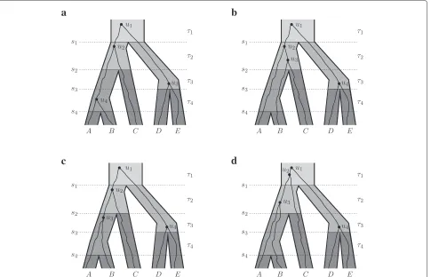
Figure 1b do not coalesce until the population ancestral to speciesA,B, andC, thus allowing theBandClineages in the gene tree to have a more recent common ancestor than lineagesAandB.

Given a fixed species tree, and assuming the gene tree evolved under the multi-species coalescent [1], the most probable gene tree topology can have a different topology from that of the species tree. Such a gene tree topology is called an anomalous gene tree. In fact, for every species tree topology with at least 5 leaves, we can choose edge lengths in the species tree topology such that anoma-lous gene trees exist [2]. This implies that the gene tree topology appearing most often when considering differ-ent genes might not agree with the species tree topology, thus we cannot use a simple majority-heuristic to infer the species tree from a collection of gene trees. Instead we need statistical tools rather than majority rule heuristics for inferring the species tree based on gene trees.

Current methods for inferring species trees from gene trees in this setting can be divided into topology-based and genealogy-topology-based methods, in which the input for a reconstruction algorithm accepts either gene tree

a

c

b

d

Figure 1In (a)–(d) the ranked species tree topology is(((A,B)₄,C)₂,(D,E)₃)₁.(a) The ranked gene tree matches the ranked species tree. (b) The (ranked or unranked) gene tree does not match the species tree, and there is an incomplete lineage sorting event (a deep coalescence) because the lineages from speciesAandBfail to coalesce more recently thans2. (c) The gene tree and species tree have the same unranked

topology but have different ranked topologies, asDandEcoalesce in the gene tree more recently thanAandB, whileAandBis the most recent divergence in the species tree. The gene tree in (c) has ranked topology(((A,B)3,C)2,(D,E)4)1. In (c), there are no incomplete lineage sorting events

(no deep coalescences); however, there is an extra lineage at times3which leads to the gene tree and species tree having different rankings. In (c),

all coalescences occur in the most recent possible interval consistent with the ranked gene tree, and we have1=2,2=3,3=5,4=5, and

g1=2,g2=3,g3=5,g4=5. (d) A gene tree with the same ranked topology as the gene tree in (c) but with coalescences occurring in different

intervals.

topologies or genealogies, i.e., gene trees with branch lengths (coalescence times). Topology-based methods include Minimize Deep Coalescence (MDC) [3,4], STAR [5], STELLS [6], rooted triple consensus [7] and other consensus and supertree methods [8,9]. Genealogy-based methods include Bayesian and likelihood methods such as BEST, *BEAST, and STEM [10-12] and clustering and distance-based methods [5,13-15]. Possible pros and cons of the two approaches are that topology-based meth-ods can be computationally faster and less sensitive to errors in estimating gene trees (and gene tree branch lengths) from sequence data [16], while methods that use coalescence times, particularly using Bayesian modelling, can be the most accurate when model assumptions are correct [17].

Another possibility that has been so far unexplored in methods for inferring species trees from gene trees is

to use ranked gene trees, in which the temporal order

of the nodes of the gene tree (the coalescence times) is used, but not the continuous-valued branch lengths. This approach might therefore be intermediate between purely topology-based methods and genealogy-based methods. By preserving more of the temporal information in the gene tree nodes, the hope is to develop methods that are more powerful than purely topology-based methods and that are still computationally efficient and robust to errors in estimating gene trees and gene tree branch lengths from sequence data.

paper, we improve this previous (computationally ineffi-cient) approach, by providing a method for computing probabilities of ranked gene trees given species trees which is polynomial in the number of leaves using a dynamic programming approach.

Methods for computing probabilities of ranked gene trees efficiently may also be of interest in the context of computing probabilities of unranked gene trees, partic-ularly because no polynomial time algorithm has been found for calculating the probability of a gene tree topol-ogy given a species tree under the multispecies coalescent [6,19-21]. The probability of an unranked gene tree topol-ogy can be obtained by summing over all ranked gene tree topologies with the same topology. Thus, for unranked gene trees with particular shapes where the number of rankings increases in polynomial time, using ranked gene trees can potentially increase the speed of computing probabilities of unranked gene trees as well. We note that a completely unbalanced gene tree has only one ranking, while the number of rankings can be exponential in the number of leaves when gene trees become more balanced. Thus, our approach for calculating unranked gene tree probabilities will be most useful for less balanced ranked gene trees.

The bulk of the paper consists of the derivation of the polynomial time method for computing ranked gene tree probabilities. The algorithm is summarized in section ‘An algorithm’. This is followed by a discussion of applications to computing probabilities of unranked gene tree topolo-gies and to inferring ranked species trees under maximum likelihood and a modification to the MDC criterion.

Calculating the probability of a ranked gene tree topology

In the following, we will derive the probability of a ranked gene tree topology given a species tree,P[G|T]. Equations (1, 2, 3, 4, 8, 10) allow the calculation of P[G|T] in timeO(n5). The model giving rise to the gene tree is the multi-species coalescent with constant popu-lation sizes [1]. Each species consists of a popupopu-lation of constant size where lineages merge according to the coa-lescent. Thus, lineages from two different species may coalesce any time previous to the split of the two species.

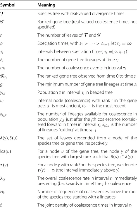
We begin with some notation, which is also summarized in Table 1. Let time be 0 today and increasing going into the past. LetT be a species tree withnspecies, and thus n−1 speciation events (denoted by 1,. . .,n−1) occur-ring at timess1>· · ·>sn−1. Denote the interval between speciation eventi− 1 and speciation event i by τ_i, see Figure 1.

LetG be a ranked gene tree topology. It is convenient to use the same labels for the leaves ofG and ofT. This is a slight abuse of notation, as leafAofT refers to a popula-tion (or species), andAofG refers to a gene sampled from

Table 1 Notation used in the paper

Symbol Meaning

T Species tree with real-valued divergence times

G Ranked gene tree (real-valued coalescence times not specified)

n The number of leaves ofT andG

si Speciation times, withs1>· · ·>sn−1, lets0= ∞

τi Intervals between speciation times,τi=[si,si−1)

i The number of gene tree lineages at timesi

mi The number of coalescence events in intervalτi Gi,i The ranked gene tree observed from time 0 to timesi

gi The minimum number of gene tree lineages at timesi

yi,z Populationzin intervalτiin beaded tree

ui Internal node (coalescence) with rankiin the gene

tree,u1is most ancient,un−1is the most recent

ki,j,z The number of lineages available for coalescence in

populationyi,zjust after thejth coalescence

(consid-ered forward in time) in intervalτi;ki,0,zis the number

of lineages “exiting” at timesi−1

δ(y),δ(u) The set of leaves descended from a node of the species tree or gene tree, respectively

lca(u) For a nodeuof the gene tree, the nodeyof the species tree with largest rank such thatδ(u)⊂δ(y) τ (y) For a nodeywith rankion the species tree, we denote

τ (y)=τi(the interval immediately abovey)

λi,j The overall coalescence rate in intervalτiimmediately

preceding (backwards in time) thejth coalescence

Hk Number of sequences of coalescences above the root

of the species tree starting withklineages

fi The joint density of coalescence times in intervalτi

populationA. We denote the nodes ofG (which are coa-lescence events) byu1,. . .,un−1, where nodeujhas rankj,

and where higher rank indicates a more recent coales-cence. A ranked tree topology can be notated similarly to Newick notation, putting the rank as a subscript for each node, see also Figure 1.

Let Gi,i be part of a ranked gene tree evolving on a species tree between timesiand time 0 (i.e. the present). Gi,iconsists ofi gene tree lineages at speciation timesi and the coalescent history ofGi,i in time interval(0,si) is consistent with the ranked gene treeG. Letgi be the

minimum number of lineages required in the ranked gene

tree at time si such that G can be embedded into the

species tree T. Note that n ≥ _i ≥ gi > i. Next we

provide a dynamic programming approach for calculat-ing the probability of a ranked gene tree given a species tree. An efficient way to determine the required quantities g1,. . .,gn−1 is provided in Section ‘Calculation ofgi and ki,j,z’.

(formalized in Theorem 2), and calculate the probability of the appropriate coalescent events occurring in

inter-val τi based on how many coalescent events happened

in the later intervals τi+1,. . .,τn−1 (Theorem 3). Finally with Theorem 1, we account for the most ancestral time intervalτ1.

Theorem 1.The probability of a ranked gene tree given a species tree is,

P[G|T]=

n

1=g1

P[G1,1|T]/H1 (1)

where

H1 =1!(1−1)!/2

1−1 ₍₂₎

is the probability for the coalescences above the root appearing in the right order[22].

For precalculatedP[G1,1|T] (1 = 2,. . .,n) the

com-plexity of calculating P[G|T] is thus O(n). Next, we will provide a recursive way to calculate P[G1,1|T] for

1 = 2,. . .,nin polynomial time, thus P[G|T] can be calculated in polynomial time.

Theorem 2.The probability P[Gi,i|T] can be

calcu-lated for all i recursively (with li≥gi),

P[Gi,i|T]

=

n

i+1=max(i,gi+1)

P[Gi,i|Gi+1,i+1,T]P[Gi+1,i+1|T]

(3)

with

P[Gn−1,n|T]=1.

The complexity of calculating P[G1,1|T] for 1 =

2,. . .,n is O(n3_{), given we knowP[G}

i,i|Gi+1,i+1,T]for all

i,i,i+1.

Proof. At the time of the most recent speciation event, sn−1, we havenlineages with probability 1, which is the initial value of the recursion. Calculating P[Gi,i|T] for

i<n−1 can be done in the following way, P[Gi,i|T]

=

n

i+1=max(i,gi+1)

P[Gi,i,Gi+1,i+1|T]

=

n

i+1=max(i,gi+1)

P[Gi,i|Gi+1,i+1,T]P[Gi+1,i+1|T] .

Suppose P[Gi,i|Gi+1,i+1,T] is known. Given we

calcu-lated the probabilityP[Gi+1,i+1|T] fori+1=i+2,. . .,n,

then calculatingP[Gi,i|T] fori = i+1,. . .,nrequires

On_j=−₁ij

= On−₂i+1 calculations. Summing up overi=1,. . .,n−1 yields a complexity ofOn_i=22i=

On+₃1=O(n3).

It remains to determinePGi−1,i−1|Gi,i,T . Note that during the intervalτ_i, we haveibranches in the species tree. Letmibe the number of coalescent events inτi, so mi = i−i−1. Let the number of lineages on branchz just after thejth coalescent event (going forward in time) inτibeki,j,z. Calculation ofki,j,zcan be done efficiently as

shown in Section ‘Calculation ofgiandki,j,z’.

Theorem 3.We have,

PGi−1,i−1|Gi,i,T =

mi

j=0

e−λi,j(si−1−si) mi

k=0,k=j(λi,k−λi,j)

(4)

whereλi,j=iz=1 _ki,j,z

2

and1₂:=0.

Proof. The density for the coalescence events in interval τ_ican be obtained by considering the waiting time to the “next” coalescent event (going backwards in time) as being due to competing exponentials in the different branches, where the coalescence rate within branchziski,j,z

2

. Thus, the waiting time until the next coalescent event has rate λi,j=iz=1

_ki,j,z 2

.

We denote the time between thejth and(j+1)st coa-lescent event asvj, wherev0is the time betweensi−1and the first (least recent) coalescent event inτiand withvmi being the time betweensiand coalescent eventmi.

The density for the coalescent events in the intervalτ_i is [18],

fi(v0,v1,. . .,vmi)=e

−mi j=0

i z=1(ki,2j,z)vj

=e− _mi

j=0λi,jvj_.

It remains to integrate overv, for which we distinguish between case (i)λi,0=0, and case (ii)λi,0>0.

Case (i): Ifλi,0 = 0 (which occurs ifi−1 = i, i.e., all lineages within each population coalesce), then we rewrite fias,

fi(v0,v1,. . .,vmi)= mi

j=1λi,je−λi,jvj mi

j=1λi,j

. (5)

Using the fact that the integral of the numerator of Equation (5) is a hypoexponential distribution based on the sum of mi exponential random variables [23] (with

density functionsλi,je−λi,jvj,j=1,. . .,mi), the probability

distribution functionof the hypoexponential distribution evaluated atsi−1−si=m_j=i₀vi. Thus, withλi,j< λi,j+1,

P[Gi−1,i−1|Gi,i,T]

= m1i

j=1λi,j

− mi

j=1

e−λi,j(si−1−si) λi,jm_k=i_1,k=j(λi,k−λi,j)

= m1i

j=1λi,j + mi

j=1

e−λi,j(si−1−si) mi

k=0,k=j(λi,k−λi,j)

= mi

j=0

e−λi,j(si−1−si) mi

k=0,k=j(λi,k−λi,j)

(6)

where the second line follows because−λi,j=λi,0−λi,j.

Case (ii): Ifλ_i,0>0, then we rewritefias,

fi(v0,v1,. . .,vmi)= mi

j=0λi,je−λi,jvj

mi

j=0λi,j

(7)

For integrating fi, we use the fact that the integral

of the numerator in Equation (7) is the convolution of

mi + 1 exponential random variables with parameters

λi,0,. . .,λi,mi, which is the hypoexponential distribution. Now, sinceλi,j < λi,j+1, we observe, using theprobability density functionof the hypoexponential distribution,

P[Gi−1,i−1|Gi,i,T]

=

v

fi(v0,v1,. . .,vmi)dv

= mi

j=0

e−λi,j(si−1−si) mi

k=0,k=j(λi,k−λi,j)

,

which is the same expression as for theλi,0 = 0 case (6). Note that for case (i) we made use of the cumulative distri-bution function of the hypoexponential distridistri-bution, while for case (ii) we made use of the density function of the hypoexponential distribution. Both cases yield the same final expression forP[Gi−1,i−1|Gi,i,T], which establishes the proof.

Corollary 4.The probabilities P[Gi−1,i−1|Gi,i,T] for

all possible i, mi andi (recall that mi = i −i−1) are calculated in O(n5), given allλi,j.

Proof.For a fixedi,miandi, we requireO(m2_i)

calcu-lations to evaluateP[Gi−1,i−1|Gi,i,T]. We need to deter-mineP[Gi−1,i−1|Gi,i,T] for all possiblei,miandi. First, we observe thati ≤ i−1 ≤n, and thus for a fixedi, we

have, 0 ≤ mi ≤ i−i. Second,i < i ≤ n. And third,

2≤i≤n−1. Thus, the number of calculations needed to calculateP[Gi−1,i−1|Gi,i,T] for all possiblei,miandiis,

O ⎛ ⎝n−1

i=2

n

i=i+1

i−i

mi=0

m2_i ⎞

⎠₌O

⎛ ⎝n−1

i=2

n

i=i+1 (_i−i)3

⎞ ⎠

=O _n−1

i=2 (n−i)4

=O(n5).

Corollary 5.The quantitiesλi,jcan be calculated for all possible i, mi,iand j in O(n5), given all ki,j,z.

Proof.For a fixedi,mi,iandj, we requireO(i)

calcu-lations to evaluate λi,j. As j = 0,. . .,mi, with the same

arguments as in Corollary 4, we obtain,

O ⎛ ⎝n−1

i=2

n

i=i+1

i−i

mi=0

mi

j=0 i

⎞

⎠₌O

⎛ ⎝n−1

i=2 i

n

i=i+1

i−i

mi=0

mi

⎞ ⎠

=O ⎛ ⎝n−1

i=2 i

n

i=i+1 (li−1)2

⎞ ⎠

=O _n−1

i=2

i(n−i)3

=O(n5).

We note that the termsP[Gi−1,i−1|Gi,i,T] are analo-gous to the functionsgi,jdefined in [24,25], which give the

probability thatilineages coalesce intojwithin timetin a single population and are used extensively in computing probabilities related to unranked gene trees [6,19,26,27]. In particular, if only one population, sayz∗, has coales-cence events, then we have r

P[Gi,i|Gi+1,i+1,T]

= gi+1,i(si−si+1)

z=z∗gki,0,z,ki,0,z(si−si+1) i+1−i

k=1

_i+1−k+1 2

,

a product ofgi,jfunctions with the denominator counting

the number of sequences in whichmicoalescences could

ranking constrains the coalescence ofAandBto be less recent than that ofDandE, so the probability for events in this interval is, r

P[G2,3|G3,5,T]=[g2,1(s2−s3)]2/2.

We illustrate that we get the same result from Theorem 3: there are two coalescence events in intervalτ3, so we use j=0, 1, 2, and calculate

λ3,0=

1 2

+

1 2

+

1 2

=0,

λ_3,1=

2 2

+

1 2

+

1 2

=1,

λ_3,2=

2 2

+

1 2

+

2 2

=2.

Thus, Equation (4) from Theorem 3 evaluates to

e−0(s2−s3)

(2−0)(1−0) +

e−1(s2−s3)

(0−1)(2−1)+

e−2(s2−s3)

(0−2)(1−2)

= 1

2 −e

−(s2−s3)+ 1

2e −2(s2−s3)

= 1

2

1−e−(s2−s3)

2

= [g2,1(s2−s3)]2/2.

Remark 6.The probability of a gene tree topology is the sum of the probabilities of each ranked gene tree with the given topology. A given tree topology has (n − 1)!/n_i=−₁1(ci−1) rankings, where ci is the number of descendant leaves of interior vertex i. A proof can be found in[28]. For a completely balanced tree on n = 2k leaves, the number of rankings grows faster than polynomial: the numerator can be approximated by,

n!≈√2πn(n/e)n,

and the denominator can be approximated by,

n−1

i=1

(ci−1)= k

i=1

(2i−1)n/2i≈nk=nlog2n_,

showing that the ratio grows faster than polynomial in n.

Calculation ofgiandki,j,z Calculation of gi

IfT andG have the same ranked topology, thengi=i+1.

In general, to computegi, we let lca(uj)be theleast com-mon ancestor node on the species tree for a nodeuj on

the ranked gene tree – i.e., the node with the largest rank on the species tree which is ancestral to all species repre-sented inuj. For a nodeyon the species tree, letτ (y)be the

interval immediately abovey. For example, in Figure 1c, τ (lca(u4))= τ3whereu4is the gene tree node with rank

4 — the node ancestral to D and E only. In order to com-pute gi, we count the number of gene tree nodes which

may occur closer to the present thansi. These are precisely

all gene tree nodesujwhere lca(uj)is in any of the

inter-valsτi+1,. . .,τn−1. Since at the present,nlineages are able to coalesce, we can expressgias,

gi=n− n−1

j=i+1

n−1

k=j

I(τ (lca(uk)) > τi) (8)

where τj < τi iff j < i, and whereI(·) is an indicator

function taking the value 1 if the condition holds and oth-erwise 0. Assuming each lca() operation isO(1)[29,30], preprocessing allows all lca terms to be computed inO(n) time. Thus, calculatingg1,. . .,gn−1can be done, based on Equation 8, inO(n3).

Calculation of ki,j,z

We let yi,j be the jth population (read left to right) in

intervalτi (equivalently, thejth branch or jth node

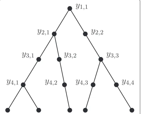
sub-tending the branch). In order to label every population before and after a speciation timesiuniquely, extra nodes

can be added to the species tree to form abeaded species tree(Figure 2), so that there are i nodes at timesi,i =

1,. . .,n−1. For eachi∈ {1,. . .,n−1}, there is one node of outdegree 2, andi−1 nodes of outdegree 1. Thus, pop-ulationyi,jcorresponds to a branch (equivalently, a node)

in the beaded species tree. We denote the outdegree of a nodeybyoutdeg(y).

In the remainder of this section, we compute the val-ueski,j,z, i.e. the number of lineages on branchyi,zof the

beaded species tree during the interval immediately after the jth coalescence event (going forward in time), with

ki,0,zbeing the number of lineages “exiting” the branch at

timesi−1. For example, in Figure 1b, we have

k2,0,1=1, k2,1,1=2, k2,2,1=3, k2,0,2=1, k2,1,2=1, k2,2,2=1,

The value ofki,j,z depends on the number of lineages

entering branch i, _i, as well as the number of lineages exiting the branch, and not just on the number of coa-lescence events in the interval. For example, in Figure 1c, k2,0,1 = 1 andk2,1,1 = 2, while in Figure 1d,k2,0,1 = 2 andk2,1,1= 3, although the two gene trees have the same ranked topology andm2=1 for both cases.

To determine the termski,j,zwe note that the number of

coalescences that have occurred more recently than inter-valτiisn−i. In a given intervalτi, we letz(1)andz(2)be

the left and right children, respectively, of populationzof outdegree 2, and letz(1)_=z(2)_{be the only child of a node}

zof outdegree 1.

The number of lineages available to coalesce in popula-tionzof intervalτ_iis

ki,mi,z=

outdeg(yi,z)

j=1

k_i+1,0,z(j) (9)

where thez(j)_{are the daughter populations (one or two)}

ofz. Further,kn,0,z =0 for allz. Since the beaded species

tree hasn2/2 nodes, precalculatingoutdeg(yi,z) requires O(n2). For 0≤j<mi, we have

ki,j,z=

ki,j+1,z−1 jth coalescence on branchz ki,j+1,z otherwise

(10)

Consequently, determining a particularki,j,zisO(1). Thus

determiningki,j,z for all possiblei,mi andi is (see also

Corollary 4),

=O ⎛ ⎝n−1

i=2

n

i=i+1

i−i

mi=0

mi

j=0 O(1)

⎞ ⎠

=O(n4).

Note that taking the sum over allzis not necessary, as in all but one branch theki,j,zequals theki,j+1,z.

An algorithm

In summary, we derived an algorithm with runtimeO(n5) for calculating the probability of a ranked gene tree given a species tree onntips:

1. Calculateg1,. . .gn−1using Equation (8).

2. Calculateki,j,z(fori,j=1,. . .,n;z=1. . .i), using Equations (9) and (10).

3. Calculateλ_i,j=

_i

z=1 ki,j,z

2

(fori,j=1,. . .,n). 4. CalculateP[Gi−1,i−1|Gi,i,T](fori=2,. . .,n;

i−1=gi−1,. . .,n;i=gi,. . .,n), using Theorem 3. 5. CalculateP[G1,1|T]using Theorem 2.

6. CalculateP[G|T]using Theorem 1.

Conclusions

In this paper, we provide a polynomial-time algorithm (O(n5)wherenis the number of species) to calculate the probability of a ranked gene tree topology given a species tree, summarized in Section ‘An algorithm’. We now dis-cuss applying these results to computing probabilities of unranked gene tree topologies and to inferring ranked species trees.

Computing probabilities of unranked gene tree topologies Previous work on computing probabilities of unranked gene tree topologies used the concept ofcoalescent his-tories, which specify the branches in the species tree in which each node of the gene tree occurs. An unranked gene tree probability can then be computed by enumerat-ing all coalescent histories and computenumerat-ing the probability of each. The number of coalescent histories grows at least exponentially when the (unranked) gene tree matches the species tree, making this approach computationally inten-sive. Coalescent histories can be enumerated either recur-sively (e.g., in PHYLONET [31] or [20]) or nonrecurrecur-sively (COAL [19]).

A much faster approach using dynamic programming similar to that used in this paper is implemented in STELLS [6], which conditions on the ancestral configura-tion in each branch rather than the number of lineages. Here an ancestral configuration keeps track not only of the number of lineages in a branch in the species tree, but also the particular nodes of the gene tree. Different ancestral configurations can potentially have the same number of lineages within a population. Enumerating ancestral con-figurations turns out to have exponential running time for arbitrarily shaped trees, but the number of ancestral con-figurations is still much smaller than the number of coa-lescent histories. When computing probabilities of ranked gene tree topologies, however, the ranking specifies the sequence of coalescence events, leading to a unique ances-tral configuration given the number of lineages in a time interval. This fortuitously enables probabilities of ranked gene tree topologies to be computed in polynomial time.

a pseudo-caterpillar, a tree made by replacing the sub-tree with four leaves of a caterpillar with a balanced sub-tree on four leaves [20], there are only two rankings possible, and for abicaterpillar[20], for which the left subtree is a caterpillar withnLleaves and the right subtree is a

cater-pillar withn−nLleaves, there are

_n−2

nL−1

rankings. Thus computing unranked gene tree probabilities by summing ranked gene tree probabilities can be done in polynomial time for some tree shapes. We note that for the approach used by STELLS, some tree shapes can also be computed in polynomial time, including the cases we mentioned with a polynomial number of rankings (caterpillar and pseudo-caterpillar). An open question is whether there are any classes of unranked gene trees which have a polyno-mial number of rankings but an exponential number of ancestral configurations, or vice versa.

Inferring species trees from ranked gene trees

Our fast calculation of the probability of ranked gene tree topologies can be used to determine the maximum likeli-hood species tree from a collection of known gene trees.

Assume we have observed N ranked gene trees (i.e.,N

loci). Now the maximum likelihood species treeTML(with

branch lengths on internal branches) is

TML=argmax

T P[G1,. . .,GN|T]

where

P[G1,. . .,GN|T]= N

k=1

P[Gk|T]=

Hn

i=1

P[G(i)|T]ni

(11)

is a multinomial likelihood. HereP[Gk|T] can be

deter-mined with our polynomial-time algorithm, we let G(i) denote theith ranked topology, andni is the number of

times ranked topologyiis observed, withHn

i=1ni = N.

Note in particular that the ranked topology ofTMLmight

differ from the most frequent ranked gene tree topology [18].

Our derivation of the ranked gene tree probability also suggests a way to infer a ranked species tree topology from ranked gene tree topologies with a similar flavor as the MDC criterion. In MDC, for an input gene tree and can-didate species tree, the number of extra lineages (lineages which necessarily fail to coalesce due to topological dif-ferences between gene and species trees) on each edge of the species tree is counted. For MDC, whether the edge of the species tree is long or short does not affect the deep coalescence cost. In working with ranked gene trees, how-ever, we can keep track of the minimum number of extra

lineages within each time intervalτi. The total number of

extra lineages in this sense is

n−1

i=1

gi−(i+1) (12)

Minimizing (12) as a criterion for the ranked species tree will tend to penalize long edges of the species tree which have multiple lineages persisting through multiple species divergence events. As an example, in Figure 1b, the gene tree has a MDC cost of 1 since there are two lineages exiting the population immediately ancestral toAandB; however the cost according (12) is 2 because there are two edges on the beaded version of the species tree (Figure 2) that each have an extra lineage. In Figure 1c, the gene tree has a MDC cost of 0 for the species tree since it has the matching unranked topology; however, the number of extra lineages from equation (12) is 1. We note that in Figure 1c, intervalτ₃, incomplete lineage sorting (and deep coalescence) have not occurred as these concepts are normally used. To capture the idea that coalescence has nevertheless occurred in a more ancient time interval than allowed, we might refer to the coalescence ofAandBin Figure 1c as an “ancient lineage sorting” event (rather than incomplete lineage sorting event) or an ancient coales-cence rather than a deep coalescoales-cence. We could therefore refer to minimizing equation (12) as the Minimize Ancient Coalescence (MAC) criterion, which would provide an interesting comparison to the usual topology-based MDC criterion.

In practice, a method of inferring a species tree from ranked gene trees would require estimating the ranked gene trees. This would require clock-like gene trees, or trees with times estimated for nodes, which can also be inferred under relaxed clock models in BEAST [32]. To account for the uncertainty in the gene trees, the counts for different ranked gene trees could be weighted by their posterior probabilities obtained from Bayesian estimation of the gene trees [33]. Thus, in equation (11), we would letnik be the posterior probability of ranked topologyiat

locusk, and useni = H_k=n₁nik as the estimated number

of times that ranked topologyi was observed. Similarly, for equation (12), the coalescence cost at a locus could be distributed over multiple topologies weighted by their posterior probabilities.

Competing interests

The authors declare that they have no competing interests.

Authors’ contributions

Both authors contributed equally to all parts of this work. Both authors read and approved the final manuscript.

Acknowledgements

and by a Sabbatical Fellowship at the National Institute for Mathematical and Biological Synthesis, an Institute sponsored by the National Science Foundation, the U.S. Department of Homeland Security, and the U.S. Department of Agriculture through NSF Award #EF-0832858, with additional support from The University of Tennessee, Knoxville. TS was funded by the Swiss National Science Foundation.

Author details

1_{Institute of Integrative Biology, Universit¨atsstrasse 16, 8092, Z ¨urich,}

Switzerland.2_{Department of Mathematics and Statistics, Private Bag 4800,} University of Canterbury, Christchurch 8140 New Zealand.3_{National Institute} of Mathematical and Biological Synthesis, Knoxville, Tennessee, USA.

Received: 30 September 2011 Accepted: 2 April 2012 Published: 30 April 2012

References

1. Degnan JH, Rosenberg NA:Gene tree discordance, phylogenetic

inference, and the multispecies coalescent.Trends Ecol Evol2009,

24:332–340.

2. Degnan JH, Rosenberg NA:Discordance of species trees with their

most likely gene trees.PLoS Genet2006,2:762–768.

3. Maddison WP, Knowles LL:Inferring phylogeny despite incomplete

lineage sorting.Syst Biol2006,55:21–30.

4. Than C, Nakhleh L:Species tree inference by minimizing deep

coalescences.PLoS Comput Biol2009,5:e1000501.

5. Liu L, Yu L, Pearl DK, Edwards SV:Estimating species phylogenies using

coalescence times among sequences.Syst Biol2009,58:468–477.

6. Wu Y:Coalescent-based species tree inference from gene tree topologies under incomplete lineage sorting by maximum

likelihood.Evolution2011, doi:10.1111/j.1558-5646.2011.01476.x.

7. Ewing GB, Ebersberger I, Schmidt HA, von Haeseler A:Rooted triple

consensus and anomalous gene trees.BMC Evol Biol2008,8:118.

8. Degnan JH, DeGiorgio M, Bryant D, Rosenberg NA:Properties of

consensus methods for inferring species trees from gene trees.Syst

Biol2009,58:35–54.

9. Wang Y, Degnan JH:Performance of matrix representation with

parsimony for inferring species from gene trees.Stat Appl Genet Mol

Biol2011,10:21.

10. Heled J, Drummond AJ:Bayesian inference of species trees from

multilocus data.Mol Biol Evol2010,27:570–580.

11. Kubatko LS, Carstens BC, Knowles LL:STEM: Species tree estimation using maximum likelihood for gene trees under coalescence. Bioinformatics2009,25:971–973.

12. Liu L, Pearl DK:Species trees from gene trees: Reconstructing bayesian posterior distributions of a species phylogeny using

estimated gene tree distributions.Syst Biol2007,56:504–514.

13. Liu L, Yu L:Estimating species trees from unrooted gene trees.Syst Biol2011,60:661–667.

14. Liu L, Yu L, Pearl DK:Maximum tree: a consistent estimator of the

species tree.J Math Biol2010,60:95–106.

15. Mossel E, Roch S:Incomplete lineage sorting: consistent phylogeny

estimation from multiple loci.IEEE/ACM Trans Comp Biol Bioinf2010,

7:166–171.

16. Huang H, He Q, Kubatko LS, Knowles LL:Sources of error for species-tree estimation: Impact of mutational and coalescent effects on accuracy and implications for choosing among different

methods.Syst Biol2009,59:573–583.

17. Liu L, Yu L, Kubatko LS, Pearl DK, Edwards SV:Coalescent methods for

estimating phylogenetic trees.Mol Phylogenet Evol2009,53:320–328.

18. Degnan JH, Rosenberg N, Stadler T:The probability distribution of

ranked gene trees on a species tree.Math Biosci2012,235:45–55.

19. Degnan JH, Salter LA:Gene tree distributions under the coalescent

process.Evolution2005,59:24–37.

20. Rosenberg NA:Counting coalescent histories.J Comput Biol2007, 14:360–377.

21. Than C, Ruths D, Innan H, Nakhleh L:Confounding factors in HGT detection: statistical error, coalescent effects, and multiple

solutions.J Comput Biol2007,14:517–535.

22. Edwards AWF:Estimation of the branch points of a branching

diffusion process.J R Stat Soc Ser B1970,32:155–174.

23. Ross S:Introduction to Probability Models. 9th ed. San Diego: Academic Press; 2007.

24. Tavar´e S:Line-of-descent and genealogical processes, and their

applications in population genetics models.Theor Popul Biol1984,

26:119–164.

25. Wakeley J:Coalescent Theory. Greenwood Village: Roberts & Company; 2008.

26. Pamilo P, Nei M:Relationships between gene trees and species trees. Mol Biol Evol1988,5:568–583.

27. Rosenberg NA:The probability of topological concordance of gene

trees and species trees.Theor Pop Biol2002,61:225–247.

28. Semple C, Steel M:Phylogenetics, vol. 24 of Oxford Lecture Series in Mathematics and its Applications. Oxford: Oxford University Press; 2003. 29. Harel D, Tarjan RE:Fast algorithms for finding nearest common

ancestors.SIAM J Comput1984,13:338–355.

30. Schiever B, Vishkin U:On finding lowest common ancestors:

simplification and parallelization.SIAM J Comput1988,17:1253–1262.

31. Than C, Ruths D, Nakhleh L:Phylonet: A software package for analyzing and reconstructing reticulate evolutionary relationships. BMC Bioinformatics2008,9:322.

32. Drummond AJ, Rambaut A:Beast: Bayesian evolutionary analysis by

sampling trees.BMC Evolut Biol2007,7:214.

33. Allman ES, Degnan JH, Rhodes JA:Identifying the rooted species tree from the distribution of unrooted gene trees under the coalescent. J Math Biol2011,62:833–862.

doi:10.1186/1748-7188-7-7

Cite this article as:Stadler and Degnan:A polynomial time algorithm for calculating the probability of a ranked gene tree given a species tree. Algorithms for Molecular Biology20127:7.

Submit your next manuscript to BioMed Central and take full advantage of:

• Convenient online submission

• Thorough peer review

• No space constraints or color figure charges

• Immediate publication on acceptance

• Inclusion in PubMed, CAS, Scopus and Google Scholar

• Research which is freely available for redistribution