R E S E A R C H
Open Access
Reducing the worst case running times of a
family of RNA and CFG problems, using Valiant
’
s
approach
Shay Zakov, Dekel Tsur and Michal Ziv-Ukelson
*Abstract
Background:RNA secondary structure prediction is a mainstream bioinformatic domain, and is key to
computational analysis of functional RNA. In more than 30 years, much research has been devoted to defining different variants of RNA structure prediction problems, and to developing techniques for improving prediction quality. Nevertheless, most of the algorithms in this field follow a similar dynamic programming approach as that presented by Nussinov and Jacobson in the late 70’s, which typically yields cubic worst case running time algorithms. Recently, some algorithmic approaches were applied to improve the complexity of these algorithms, motivated by new discoveries in the RNA domain and by the need to efficiently analyze the increasing amount of accumulated genome-wide data.
Results:We study Valiant’s classical algorithm for Context Free Grammar recognition in sub-cubic time, and extract features that are common to problems on which Valiant’s approach can be applied. Based on this, we describe several problem templates, and formulate generic algorithms that use Valiant’s technique and can be applied to all problems which abide by these templates, including many problems within the world of RNA Secondary Structures and Context Free Grammars.
Conclusions:The algorithms presented in this paper improve the theoretical asymptotic worst case running time bounds for a large family of important problems. It is also possible that the suggested techniques could be applied to yield a practical speedup for these problems. For some of the problems (such as computing the RNA partition function and base-pair binding probabilities), the presented techniques are the only ones which are currently known for reducing the asymptotic running time bounds of the standard algorithms.
1 Background
RNA research is one of the classical domains in bioin-formatics, receiving increasing attention in recent years due to discoveries regarding RNA’s role in regulation of genes and as a catalyst in many cellular processes [1,2]. It is well-known that the function of an RNA molecule is heavily dependent on its structure [3]. However, due to the difficulty ofphysicallydetermining RNA structure
via wet-lab techniques, computational prediction of
RNA structures serves as the basis of many approaches related to RNA functional analysis [4]. Most computa-tional tools for RNA structural prediction focus on RNA
secondary structures - a reduced structural
representation of RNA molecules which describes a set of paired nucleotides, through hydrogen bonds, in an RNA sequence. RNA secondary structures can be rela-tively well predicted computationally in polynomial time (as opposed to three-dimensional structures). This com-putational feasibility, combined with the fact that RNA secondary structures still reveal important information about the functional behavior of RNA molecules, account for the high popularity of state-of-the-art tools for RNA secondary structure prediction [5].
Over the last decades, several variants of RNA second-ary structure prediction problems were defined, to which polynomial algorithms have been designed. These variants include the basicRNA foldingproblem (predict-ing the secondary structure of a s(predict-ingle RNA strand
which is given as an input) [6-8], the RNA-RNA
* Correspondence: michaluz@cs.bgu.ac.il
Department of Computer Science, Ben-Gurion University of the Negev, P.O.B. 653 Beer Sheva, 84105, Israel
Interaction problem (predicting the structure of the complex formed by two or more interacting RNA mole-cules) [9], the RNA Partition Function and Base Pair
Binding Probabilitiesproblem of a single RNA strand
[10] or an RNA duplex [11,12] (computing the pairing probability between each pair of nucleotides in the input), the RNA Sequence to Structured-Sequence
Align-mentproblem (aligning an RNA sequence to sequences
with known structures) [13,14], and the RNA
Simulta-neous Alignment and Folding problem (finding a
sec-ondary structure which is conserved by multiple homologous RNA sequences) [15]. Sakakibara et al. [16] noticed that the basic RNA Foldingproblem is in fact a
special case of the Weighted Context Free Grammar
(WCFG) Parsing problem (also known asStochasticor
Probabilistic CFG Parsing) [17]. Their approach was
then followed by Dowell and Eddy [18], Do et al. [19], and others, who studied different aspects of the relation-ship between these two domains. The WCFG Parsing problem is a generalization of the simpler non-weighted
CFG Parsingproblem. Both WCFG and CFG Parsing
problems can be solved by the Cocke-Kasami-Younger (CKY) dynamic programming algorithm [20-22], whose running time is cubic in the number of words in the input sentence (or in the number of nucleotides in the input RNA sequence).
The CFG literature describes two improvements which allow to obtain a sub-cubic time for the CKY algorithm. The first among these improvements was a technique suggested by Valiant [23], who showed that the CFG
Parsing problem on a sentence with n words can be
solved in a running time which matches the running time of a Boolean Matrix Multiplication of two n ×n matrices. The current asymptotic running time bound for this variant of matrix multiplication was given by Coppersmith-Winograd [24], who showed an O(n2.376) time (theoretical) algorithm. In [25], Akutsu argued that the algorithm of Valiant can be modified to deal also with WCFG Parsing (this extension is described in more details in [26]), and consequentially with RNA Folding. The running time of the adapted algorithm is different from that of Valiant’s algorithm, and matches the
run-ning time of aMax-Plus Multiplication of two n× n
matrices. The current running time bound for this
var-iant isOn3log3logn log2n
, given by Chan [27].
The second improvement to the CKY algorithm was introduced by Graham et al. [28], who applied theFour
Russians technique [29] and obtained anO
n3 logn
run-ning time algorithm for the (non-weighted) CFG Parsing problem. To the best of our knowledge, no extension of this approach to the WCFG Parsing problem has been described. Recently, Frid and Gusfield [30] showed how
to apply the Four Russianstechnique to the RNA fold-ing problem (under the assumption of a discrete scorfold-ing scheme), obtaining the same running time ofOlogn3n.
This method was also extended to deal with the RNA simultaneous alignment and folding problem [31],
yield-ing anO
n6 logn
running time algorithm.
Several other techniques have been previously devel-oped to accelerate the practical running times of differ-ent variants of CFG and RNA related algorithms. Nevertheless, these techniques either retain the same worst case running times of the standard algorithms [14,28,32-36], or apply heuristics which compromise the optimality of the obtained solutions [25,37,38]. For some
of the problem variants, such as the RNA Base Pair
Binding Probabilities problem (which is considered to
be one of the variants that produces more reliable pre-dictions in practice), no speedup to the standard algo-rithms has been previously described.
In his paper [23], Valiant suggested that his approach could be extended to additional related problems. How-ever, in more than three decades which have passed since then, very few works have followed. The only extension of the technique which is known to the
authors is Akutsu’s extension to WCFG Parsing and
RNA Folding [25,26]. We speculate that simplifying Valiant’s algorithm would make it clearer and thus more accessible to be applied to a wider range of problems.
Indeed, in this work we present a simple description of Valiant’s technique, and then further generalize it to cope with additional problem variants which do not fol-low the standard structure of CFG/WCFG Parsing (a preliminary version of this work was presented in [39]). More specifically, we define three template formulations, entitledVector Multiplication Templates (VMTs). These templates abstract the essential properties that charac-terize problems for which a Valiant-like algorithmic approach can yield algorithms of improved time com-plexity. Then, we describe generic algorithms for all pro-blems sustaining these templates, which are based on Valiant’s algorithm.
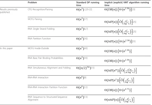
Table 1 lists some examples of VMT problems. The table compares between the running times of standard dynamic programming (DP) algorithms, and the VMT algorithms presented here. In the single string problems, ndenotes the length of the input string. In the double-string problems [9,12,13], both input double-strings are
assumed to be of the same length n. For the RNA
Simultaneous Alignment and Folding problem, m
O(n2.376), due to Coppersmith and Winograd [24]. MP (n) denotes the time complexity of a Min-Plus or a
Max-Plus Multiplication of two n × n matrices, for
which the current best theoretical result is
On3log3logn log2n
, due to Chan [27]. For most of the pro-blems, the algorithms presented here obtain lower run-ning time bounds than the best algorithms previously known for these problems. It should be pointed out that the above mentioned matrix multiplication running times are the theoretical asymptotic times for suffi-ciently large matrices, yet they do not reflect the actual multiplication time for matrices of realistic sizes. Never-theless, practical fast matrix multiplication can be obtained by using specialized hardware [40,41] (see Sec-tion 6).
The formulation presented here has several advantages over the original formulation in [23]: First, it is consid-erably simpler, where the correctness of the algorithms follows immediately from their descriptions. Second, some requirements with respect to the nature of the problems that were stated in previous works, such as operation commutativity and distributivity requirements
in [23], or thesemiringdomain requirement in [42], can be easily relaxed. Third, this formulation applies in a natural manner to algorithms for several classes of pro-blems, some of which we show here. Additional problem variants which do not follow the exact templates pre-sented here, such as the formulation in [12] for the RNA-RNA Interaction Partition Function problem, or the formulation in [13] for the RNA Sequence to Struc-tured-Sequence Alignment problem, can be solved by introducing simple modifications to the algorithms we present. Interestingly, it turns out that almost every var-iant of RNA secondary structure prediction problem, as well as additional problems from the domain of CFGs, sustain the VMT requirements. Therefore, Valiant’s technique can be applied to reduce the worst case run-ning times of a large family of important problems. In general, as explained later in this paper, VMT problems are characterized in that their computation requires the execution of many vector multiplication operations, with respect to different multiplication variants (Dot Product,
Boolean Multiplication, andMin/Max Plus
Multiplica-tion). Naively, the time complexity of each vector
Table 1 Time complexities of several VMT problems
Problem Standard DP running
time
Implicit [explicit] VMT algorithm running time
Results previously published
CFG Recognition/Parsing (n3)) [20-22] (DB(n))n2.38[23]
WCFG Parsing (n3)[17]
(MP(n))
˜ O
n3 log2n [25]
RNA Single Strand Folding (n3)[6,7]
(MP(n))O˜ n3 log2n [25]
RNA Partition Function (n3)[10]
(MP(n))n2.38[25]
In this paper WCFG Inside-Outside (n3)[43]
(DB(n))n2.38
RNA Base Pair Binding Probabilities (n3)[10]
(DB(n))n2.38
RNA Simultaneous Alignment and Folding ((n/2)3m)[15]
(MP(nm))O˜ n3m mlog2n
RNA-RNA Interaction (n6)[9]
(MP(n2))
˜ O
n6 log2n
RNA-RNA Interaction Partition Function (n6)[12]
(DB(n))n4.75
RNA Sequence to Structured-Sequence
Alignment (n
4)[13]
(nMP(n))O˜ n4 log2n
multiplication is linear in the length of the multiplied vectors. Nevertheless, it is possible to organize these vector multiplications as parts of square matrix multipli-cations, and to apply fast matrix multiplication algo-rithms in order to obtain a sub-linear (amortized) running time for each vector multiplication. As we show, a main challenge in algorithms for VMT pro-blems is to describe how to bundle subsets of vector multiplications operations in order to compute them via the application of fast matrix multiplication algorithms. As the elements of these vectors are computed along the run of the algorithm, another aspect which requires attention is the decision of the order in which these matrix multiplications take place.
Road Map
In Section 2 the basic notations are given. In Section 3 we describe theInside Vector Multiplication Template- a template which extracts features for problems to which Valiant’s algorithm can be applied. This section also includes the description of an exemplary problem (Section 3.1), and a generalized and simplified exhibition of Vali-ant’s algorithm and its running time analysis (Section 3.3). In Sections 4 and 5 we define two additional problem tem-plates: theOutside Vector Multiplication Template, and theMultiple String Vector Multiplication Template, and describe modifications to the algorithm of Valiant which allow to solve problems that sustain these templates. Sec-tion 6 concludes the paper, summarizing the main results and discussing some of its implications. Two additional exemplary problems (an Outside and a Multiple String VMT problems) are presented in the Appendix.
2 Preliminaries
As intervals of integers, matrices, and strings will be extensively used throughout this work, we first define some related notation.
2.1 Interval notations
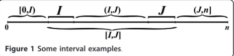
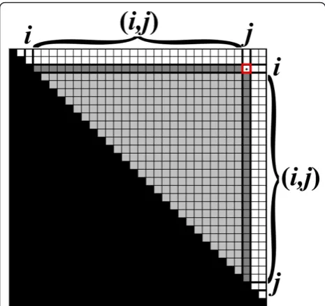
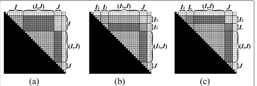
For two integersa, b, denote by [a,b] the interval which contains all integers q such that a ≤ q ≤ b. For two intervalsI = [i1, i2] andJ = [j1,j2], define the following intervals: [I,J] = {q: i1≤q ≤j2}, (I,J) = {q: i2< q < j1}, [I,J) = {q: i1 ≤q < j1}, and (I, J] = {q :i2 < q≤ j2} (Fig-ure 1). When an integerr replaces one of the intervalsI or Jin the notation above, it is regarded as the interval
[r,r]. For example, [0,I) = {q: 0≤q < i1}, and (i,j) = {q : i < q < j}. For two intervalsI= [i1, i2] and J = [j1,j2] such that j1 =i2 + 1, define IJ to be the concatenation ofIand J, i.e. the interval [i1,j2].
2.2 Matrix notations
LetX be ann1 ×n2matrix, with rows indexed with 0, 1, ..., n1 - 1 and columns indexed with 0, 1, ..., n2 - 1. Denote byXi, jthe element in the ith row andjth col-umn of X. For two intervals I⊆[0,n1) and J⊆ [0,n2), letXI,Jdenote the sub-matrix ofX obtained by project-ing it onto the subset of rowsIand subset of columnsJ. Denote by Xi, J the sub-matrixX[i,i],J, and by XI, j the sub-matrix XI,[j,j]. LetDbe a domain of elements, and⊗ and⊕be two binary operations onD. We assume that (1)⊕is associative (i.e. for three elementsa,b,cin the domain, (a⊕b)⊕c=a⊕(b⊕c)), and (2) there exists
a zero element j in D, such that for every element
a∈Da⊕j=j⊕a=aanda⊗j=j⊗a=j. LetXandYbe a pair of matrices of sizesn1×n2andn2×
n3, respectively, whose elements are taken fromD. Define the result of thematrix multiplication X⊗Yto be the matrixZof sizen1×n3, where each entryZi,jis given by
Zi,j=⊕q∈[0,n2)(Xi,q⊗Yq,j) = (Xi,0⊗Y0,j)⊕(Xi,1⊗Y1,j)⊕. . .⊕(Xi,n2−1⊗Yn2−1,j).
In the special case where n2 = 0, define the result of the multiplication Z to be an n1 ×n3 matrix in which all elements arej. In the special case wheren1 =n3 = 1, the matrix multiplication X⊗Yis also called avector multiplication (where the resulting matrixZ contains a single element).
Let X and Y be two matrices. When X and Yare of
the same size, define the result of thematrix addition X
⊕ Yto be the matrix Z of the same size as X and Y, where Zi, j=Xi,j⊕Yi, j. When XandYhave the same
number of columns, denote by
X Y
the matrix obtained
by concatenating Y below X. WhenX and Yhave the
same number of rows, denote by [XY] the matrix
obtained by concatenatingYto the right ofX. The fol-lowing properties can be easily deduced from the defini-tion of matrix multiplicadefini-tion and the associativity of the
⊕operation (in each property the participating matrices are assumed to be of the appropriate sizes).
X1 X2
⊗Y =
X1⊗Y X2⊗Y
(1)
X⊗[Y1Y2] = [(X⊗Y1)(X⊗Y2)] (2)
(X1⊗Y1)⊕(X2⊗Y2) = [X1X2]⊗
Y1 Y2
(3)
Under the assumption that the operations ⊗and ⊕
between two domain elements consumeΘ(1)
computa-tion time, a straightforward implementacomputa-tion of a matrix multiplication between twon×nmatrices can be com-puted inΘ(n3) time. Nevertheless, for some variants of multiplications, sub-cubic algorithms for square matrix multiplications are known. Here, we consider three such variants, which will be referred to asstandard multipli-cationsin the rest of this paper:
• Dot Product: The matrices hold numerical
ele-ments,⊗stands for number multiplication (·) and⊕ stands for number addition (+). Thezero element is 0. The running time of the currently fastest algo-rithm for this variant isO(n2.376) [24].
• Min-Plus/Max-Plus Multiplication: The matrices
hold numerical elements,⊗stands for number addi-tion and⊕stands for min or max (whereaminbis
the minimum between a and b, and similarly for
max). The zero element is∞for the Min-Plus var-iant and -∞ for the Max-Plus variant. The running time of the currently fastest algorithm for these
var-iants isO
n3log3 logn log2n
[27].
•Boolean Multiplication: The matrices hold boolean
elements, ⊗ stands for boolean AND (⋀) and ⊕
stands for boolean OR(⋁). The zeroelement is the
false value. Boolean Multiplication is computable
with the same complexity as the Dot Product, having the running time of O(n2.376) [24].
2.3 String notations
Let s =s0s1 ... sn- 1 be a string of length n over some alphabet. Aposition q insrefers to a point between the characterssq - 1andsq(a position may be visualized as a vertical line which separates between these two char-acters). Position 0 is regarded as the point just befores0, and positionnas the point just aftersn- 1. Denote by ||
s|| = n + 1 the number of different positions in s. Denote bysi,jthe substring ofsbetween positionsiand
j, i.e. the string sisi+1...sj- 1. In a case wherei=j, si, j corresponds to an empty string, and fori > j, si, j does not correspond to a valid string.
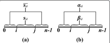
An inside property bi,j is a property which depends only on the substring si, j(Figure 2). In the context of RNA, an input string usually represents a sequence of nucleotides, where in the context of CFGs, it usually represents a sequence of words. Examples of inside properties in the world of RNA problems are the maxi-mum number of base-pairs in a secondary structure of si,j [6], the minimum free energy of a secondary struc-ture of si, j [7], the sum of weights of all secondary structures of si, j [10], etc. In CFGs, inside properties
can be boolean values which state whether the sub-sen-tence can be derived from some non-terminal symbol of the grammar, or numeric values corresponding to the weight of (all or best) such derivations [17,20-22].
Anoutside property ai,j is a property of the residual string obtained by removingsi, jfrom s(i.e. the pair of stringss0,iandsj,n, see Figure 2). Such a residual string is denoted bysi,j. Outside property computations occur in algorithms for the RNA Base Pair Binding Probabil-ities problem [10], and in the Inside-Outside algorithm for learning derivation rule weights for WCFGs [43].
In the rest of this paper, given an instance string s, substrings of the form si, jand residual strings of the form si,j will be considered assub-instances of s. Char-acters and positions in such sub-instances are indexed according to the same indexing as of the original string s. That is, the characters in sub-instances of the form si, jare indexed fromi toj- 1, and in sub-instances of the form si,j the first i characters are indexed between 0 and i - 1, and the remaining characters are indexed
between j and n - 1. The notation b will be used to
denote the set of all values of the formbi,jwith respect to substringssi, j of some given strings. It is conveni-ent to visualize bas an ||s|| × ||s|| matrix, where the (i, j)-th entry in the matrix contains the valuebi,j. Only entries in the upper triangle of the matrix b corre-spond to valid substrings of s. For convenience, we define that values of the formbi,j, when j < i, equal to
j (with respect to the corresponding domain of
values). Notations such asbI, J, bi, J, andbI, j are used in order to denote the corresponding sub-matrices of
b, as defined above. Similar notations are used for a set aof outside properties.
3 The Inside Vector Multiplication Template
In this section we describe a template that defines a class of problems, called theInside Vector Multiplication
Template (Inside VMT). We start by giving a simple
motivating example in Section 3.1. Then, the class of Inside VMT problems is formally defined in Section 3.2, and in Section 3.3 an efficient generic algorithm for all Inside VMT problems is presented.
3.1 Example: RNA Base-Pairing Maximization
The RNA Base-Pairing Maximizationproblem [6] is a
simple variant of theRNA Folding problem, and it exhi-bits the main characteristics of Inside VMT problems. In this problem, an input strings =s0s1 ...sn- 1 repre-sents a string ofbases(ornucleotides) over the alphabet A, C, G, U. Besides strong (covalent) chemical bonds which occur between each pair of consecutive bases in the string, bases at distant positions tend to form addi-tional weaker (hydrogen) bonds, where a base of typeA can pair with a base of typeU, a base of typeCcan pair with a base of type G, and in addition a base of typeG can pair with a base of type U. Two bases which can pair to each other in such a (weak) bond are called com-plementary bases, and a bond between two such bases is called abase-pair. The notationa•b is used to denote that the bases at indices aandb insare paired to each other.
A folding(or asecondary structure) of s is a setF of base-pairs of the form a • b, where 0 ≤ a < b < n, which sustains that there are no two distinct base pairs a•b andc•dinFsuch thata≤c≤b ≤d(i.e. the par-ing is nested, see Figure 3). Denote by |F| the number of
complementary base-pairs in F. The goal of the RNA
base-paring maximization problem is to compute the maximum number of complementary base-pairs in a folding of an input RNA strings. We call such a num-ber the solutionfor s, and denote by bi, jthe solution for the substringsi,j. For substrings of the formsi, iand
si,i+1 (i.e. empty strings or strings of length 1), the only possible folding is the empty folding, and thusbi,i=bi,
i+1= 0. We next explain how to recursively computebi,
jwhenj > i + 1.
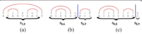
In order to compute values of the formbi,j, we distin-guish between two types of foldings for a substringsi, j: foldings of typeIare those which contain the base-pair i•(j- 1), and foldings of typeIIare those which do not containi•(j- 1).
Consider a foldingFof typeI. Sincei•(j- 1) ÎF, the foldingF is obtained by adding the base-pairi •(j - 1) to some foldingF’for the substringsi+1,j- 1(Figure 3a). The number of complementary base-pairs in Fis thus | F’| + 1 if the bases siandsj- 1are complementary, and otherwise it is |F’|. Clearly, the number of complemen-tary base-pairs inFis maximized when choosingF’such that |F’| =bi+1,j- 1. Now, Consider a foldingFof type
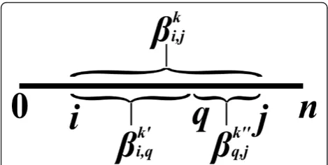
II. In this case, there must exist some positionqÎ (i,j), such that no base-pair a•b in Fsustains that a < q≤ b. This observation is true, since if j - 1 is paired to some indexp(where i < p < j- 1), then q =psustains the requirement (Figure 3b), and otherwiseq=j- 1 sus-tains the requirement (Figure 3c). Therefore,q splitsF into two independent foldings: a foldingF’for the prefix si,q, and a foldingF” for the suffixsq, j, where |F| = |F’| + |F”|. For a specific split position q, the maximum number of complementary base-pairs in a folding of typeII forsi, jis then given bybi, q +bq, j, and taking the maximum over all possible positionsqÎ (i,j) guar-antees that the best solution of this form is found.
Thus,bi, jcan be recursively computed according to the following formula:
βi,j= max
(I) βi+1,j−1+δi,j−1,
(II) max
q∈(i,j){βi,q+βq,j}
,
where δi, j - 1 = 1 if si and sj - 1 are complementary bases, and otherwiseδi,j- 1= 0.
3.1.1 The classical algorithm
The recursive computation above can be efficiently implemented using dynamic programming (DP). For an input string s of length n, the DP algorithm maintains the upper triangle of an ||s|| × ||s|| matrixB, where each entry Bi,j inBcorresponds to a solutionbi, j. The entries in B are filled, starting from short base-case entries of the form Bi, i and Bi,i+1, and continuing by computing entries corresponding to substrings with increasing lengths. In order to compute a value bi, j according to the recurrence formula, the algorithm needs to examine only values of the form bi’,j’such that
si’,j’is a strict substring ofsi,j(Figure 4). Due to the bot-tom-up computation, these values are already computed
and stored in B, and thus each such value can be
obtained inΘ(1) time.
Upon computing a valuebi, j, the algorithm needs to compute term (II) of the recurrence. This computation is of the form of avector multiplication operation⊕qÎ(i, j)(bi, q⊗bq, j), where the multiplication variant is the
Max Plusmultiplication. Since all relevant values in B are computed, this computation can be implemented by computingBi, (i,j)⊗B(i,j),j(the multiplication of the two darkened vectors in Figure 4), which takesΘ(j-i) run-ning time. After computing term (II), the algorithm
Figure 3An RNA string s=s0,9= ACAGUGACU, and three corresponding foldings. (a) A folding of typeI, obtained by adding the base-pairi•(j- 1) = 0•8 to a folding forsi+1,j-1=s1,8.
(b) A folding of typeII, in which the last index 8 is paired to index 6. The folding is thus obtained by combining two independent foldings: one for the prefixs0,6, and one for the suffixs6,9. (c) A
folding of typeII, in which the last index 8 is unpaired. The folding is thus obtained by combining a folding for the prefixs0,8, and an
needs to perform additional operations for computingbi,
jwhich takeΘ(1) running time (computing term (I), and taking the maximum between the results of the two terms). It can easily be shown that, on average, the run-ning time for computing each valuebi, j isΘ(n), and thus the overall running time for computing all Θ(n2) values bi, j is Θ(n3). Upon termination, the computed matrix Bequals to the matrix b, and the required result
b0,nis found in the entryB0,n.
3.2 Inside VMT definition
In this section we characterize the class of Inside VMT
problems. TheRNA Base-Paring Maximizationproblem,
which was described in the previous section, exhibits a simple special case of an Inside VMT problem, in which the goal is to compute a single inside property for a given input string. Note that this requires the computa-tion of such inside properties for all substrings of the input, due to the recursive nature of the computation. In other Inside VMT problems the case is similar, hence we will assume that the goal of Inside VMT problems is to compute inside properties for allsubstrings of the input string. In the more general case, an Inside VMT problem defines several inside properties, and all of these properties are computed for each substring of the input in a mutually recursive manner. Examples of such problems are the RNA Partition Function problem [10]
(which is described in Appendix A), the RNA Energy
Minimizationproblem [7] (which computes several fold-ing scores for each substrfold-ing of the input, correspondfold-ing
to restricted types of foldings), and the CFG Parsing problem [20-22] (which computes, for every non-term-inal symbol in the grammar and every sub-sentence of the input, a boolean value that indicates whether the sub-sentence can be derived in the grammar when start-ing the derivation from the non-terminal symbol).
A common characteristic of all Inside VMT problems is that the computation of at least one type of an inside property requires a result of a vector multiplication operation, which is of similar structure to the multipli-cation described in the previous section for the RNA Base-Paring Maximization problem. In many occasions, it is also required to output a solutionthat corresponds to the computed property, e.g. a minimum energy sec-ondary structure in the case of the RNA folding pro-blem, or a maximum weight parse-tree in the case of the WCFG Parsing problem. These solutions can usually be obtained by applying a traceback procedure over the computed dynamic programming tables. As the running times of these traceback procedures are typically negligi-ble with respect to the time needed for filling the values in the tables, we disregard this phase of the computation in the rest of the paper.
The following definition describes the family ofInside
VMT problems, which share common combinatorial
characteristics and may be solved by a generic algorithm which is presented in Section 3.3.
Definition 1A problem is considered an Inside VMT
problemif it fulfills the following requirements.
1. Instances of the problem are strings, and the goal of the problem is to compute for every substring si, j
of an input string s, a series of inside properties
β1
i,j, βi2,j, . . ., βiK,j.
2. Let si,jbe a substring of some input string s. Let 1
≤k≤K, and letμki,jbe a result of a vector multiplica-tion of the formμki,j=⊕q∈(i,j)
βk i,q⊗βk
q,j
, for some 1
≤k’, k” ≤ K. Assume that the following values are available:μki,j, all valuesβik,jfor 1≤k’≤K and si’,j’a
strict substring of si,j, and all valuesβk
i,jfor1≤ k’< k. Then,βik,jcan be computed in o(||s||) running time. 3. In the multiplication variant that is used for com-putingμki,j, the ⊕operation is associative, and the domain of elements contains a zero element. In addi-tion, there is a matrix multiplication algorithm for this multiplication variant, whose running time M(n) over two n×n matrices satisfies M(n) =o(n3).
Intuitively,μki,jreflects an expression which examines all possible splits ofsi, jinto a prefix substringsi,q and a suffix substringsq, j(Figure 5). Each split corresponds to
Figure 4The tableBmaintained by the DP algorithm. In order to computeBi,j, the algorithm needs to examine only values in
a term that should be considered when computing the propertyβik,j, where this term is defined to be the
appli-cation of the ⊗operator between the propertyβik,qof the prefix si, q, and the propertyβk
q,jof the suffix sq, j (where ⊗usually stands for +, ·, or ⋀). The combined valueμki,jfor all possible splits is then defined by apply-ing the ⊕operation (usually min/max, +, or ⋁) over these terms, in a sequential manner. The template allows examiningμki,j, as well as additional values of the formβik,j, for strict substrings si’,j’of si, jand 1 ≤ k’ <K, and values of the formβik,jfor 1 ≤ k’ < k, in order to compute βik,j. In typical VMT problems (such as the RNA Base-Paring Maximization problem, and excluding problems which are described in Section 5), the algo-rithm needs to performΘ(1) operations for computing βk
i,j, assuming that μki,jand all other required values are pre-computed. Nevertheless, the requirement stated in the template is less strict, and it is only assumed that this computation can be executed in a sub-linear time with respect to ||s||.
3.3 The Inside VMT algorithm
We next describe a generic algorithm, based on Vali-ant’s algorithm [23], for solving problems sustaining the Inside VMT requirements. For simplicity, it is assumed that a single property bi, j needs to be computed for each substringsi,jof the input strings. We later explain how to extend the presented algorithm to the more gen-eral cases of computing K inside properties for each substring.
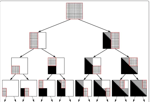
The new algorithm also maintains a matrix B as
defined in Section 3.1. It is a divide-and-conquer recur-sive algorithm, where at each recurrecur-sive call the algo-rithm computes the values in a sub-matrix BI, J of B (Figure 6). The actual computation of values of the form
bi, j is conducted at the base-cases of the recurrence, where the corresponding sub-matrix contains a single entry Bi, j. The main idea is that upon reaching this
stage the termμi,jwas already computed, and thusbi, j can be computed efficiently, as implied by item 2 of Definition 1. The accelerated computation of values of the form μi, j is obtained by the application of fast matrix multiplication subroutines between sibling recur-sive calls of the algorithm. We now turn to describe this process in more details.
At each stage of the run, each entryBi, jeither con-tains the valuebi,j, or some intermediate result in the computation ofμi, j. Note that only the upper triangle of
B corresponds to valid substrings of the input. Never-theless, our formulation handles all entries uniformly, implicitly ignoring values in entries Bi,jwhenj < i. The following pre-condition is maintained at the beginning of the recursive call for computingBI, J(Figure 7):
1. Each entryBi, jinB[I,J], [I,J]contains the valuebi, j, except for entries inBI,J.
2. Each entryBi, jin BI,J contains the value⊕qÎ(I,J) (bi, q⊗bq,j). In other words,BI,J =bI,(I,J)⊗b(I,J),J.
Letndenote the length ofs. Upon initialization,I=J = [0,n], and all values inBare set toj. At this stage (I, J) is an empty interval, and so the pre-condition with respect to the complete matrixB is met. Now, consider a call to the algorithm with some pair of intervalsI,J. If I= [i,i] and J = [j,j], then from the pre-condition, all valuesbi’,j’which are required for the computationbi, j of are computed and stored inB, andBi,j=μi,j(Figure 4). Thus, according to the Inside VMT requirements,bi,
jcan be evaluated ino(||s||) running time, and be stored inBi,j.
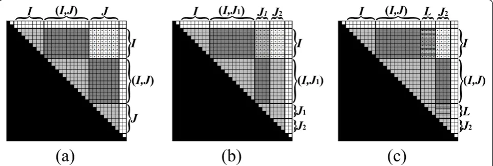
Else, either |I| >1 or |J|>1 (or both), and the algo-rithm partitionsBI, J into two sub-matrices of approxi-mately equal sizes, and computes each part recursively. This partition is described next. In the case where |I|
≤ |J|, BI,J is partitioned vertically (Figure 8). Let J1 and
J2 be two column intervals such thatJ =J1J2 and |J1| =
⌊|J|/2⌋ (Figure 8b). Since J and J1 start at the same index, (I, J) = (I, J1). Thus, from the pre-condition and Equation 2, BI,J1 =βI,(I,J1)⊗β(I,J1),J1. Therefore, the pre-condition with respect to the sub-matrix BI,J1is met, and the algorithm computes this sub-matrix recur-sively. AfterBI,J1is computed, the first part of the pre-condition with respect to BI,J2is met, i.e. all necessary values for computing values in BI,J2, except for those in
BI,J2itself, are computed and stored in B. In addition, at this stageBI,J2=βI,(I,J)⊗β(I,J),J2. LetLbe the interval such that (I, J2) = (I, J)L. Lis contained in J1, where it can be verified that either L= J1 (if the last index in I is smaller than the first index in J, as in the example of Figure 8c), or L is an empty interval (in all other cases which occur along the recurrence). To meet the full pre-condition requirements with respect to I and
J2, BI,J2 is updated using Equation 3 to be BI,J2⊕(BI,L⊗BL,J2) =
βI,(I,J)⊗β(I,J),J2
⊕βI,L⊗βL,J2
=βI,(I,J2)⊗β(I,J2),J2. Now, the pre-condition with respect toBI,J2is estab-lished, and the algorithm computesBI,J2recursively. In the case where |I|>|J|, BI,J is partitioned horizontally, in a symmetric manner to the vertical partition. The horizontal partition is depicted in Figure 9. The com-plete pseudo-code for the Inside VMT algorithm is given in Table 2.
3.3.1 Time complexity analysis for the Inside VMT algorithm In order to analyze the running time of the presented algorithm, we count separately the time needed for computing the base-cases of the recurrence, and the time for non-base-cases.
In the base-cases of the recurrence (lines 1-2 in Proce-dure Compute-Inside-Sub-Matrix, Table 2), |I| = |J| = 1, and the algorithm specifically computes a value of the form bi,j. According to the VMT requirements, each such value is computed in o(||s||) running time. Since
there areΘ(||s||2) such base-cases, the overall running time for their computation iso(||s||3).
Next, we analyze the time needed for all other parts of the algorithm except for those dealing with the base-cases. For simplicity, assume that ||s|| = 2x for some integerx. Then, due to the fact that at the beginning |I| = |J| = 2x, it is easy to see that the recurrence encoun-ters pairs of intervals I,J such that either |I| = |J| or |I| = 2|J|.
Denote by T(r) andD(r) the time it takes to compute all recursive calls (except for the base-cases) initiated from a call in which |I| = |J| =r (exemplified in Figure 8) and |I| = 2|J| = r (exemplified in Figure 9), respectively.
When |I| = |J| =r (lines 4-9 in Procedure Compute-Inside-Sub-Matrix, Table 2), the algorithm performs two recursive calls with sub-matrices of sizer× r2, a matrix multiplication between anr×2r and an 2r ×2r matrices, and a matrix addition of twor× r
2matrices. Since the
matrix multiplication can be implemented by perform-ing two2r × 2r matrix multiplications (Equation 1),T (r) is given by
T(r) = 2D(r) + 2M r
2
+(r2).
When |I| = 2|J| =r (lines 10-15 in Procedure Com-pute-Inside-Sub-Matrix, Table 2), the algorithm per-forms two recursive calls with sub-matrices of size r
2× r
2, a matrix multiplication between two
r 2×
r 2 matrices, and a matrix addition of two 2r ×2r matrices. Thus,D(r) is given by
D(r) = 2Tr 2
+M r
2
+(r2).
Therefore,T(r) = 4T(r 2) + 4M(
r 2) +(r
2). By the mas-ter theorem[44],T(r) is given by
•T(r) =Θ(r2logk+1r), ifM(r) =O(r2logkr) for somek
≥0, and
•T(r) =(M(r2)), if M(2r) =(r2+ε)for some ε>0, and 4M(2r)≤dM(r)for some constant d <1 and sufficiently larger.
The running time of all operations except for the computations of base cases is thusT(||s||). In both cases listed above,T(||s||) = o(||s||3), and therefore the over-all running time of the algorithm is sub-cubic running time with respect to the length of the input string.
The currently best algorithms for the three standard multiplication variants described in Section 2.2 satisfy that M(r) = Ω(r2+ε), and imply that T(r) =Θ(M(r)). When this case holds, and the time complexity of com-puting the base-cases of the recurrence does not exceed M(||s||) (i.e. when the amortized running time for
com-puting each one of the Θ(||s||2) base cases is
OM||(s||||s2||)
), we say that the problem sustains the
stan-dard VMT settings. The running time of the VMT
algo-rithm over such problems is thus Θ (M(||s||)). All realistic inside VMT problems familiar to the authors sustain the standard VMT settings.
3.3.2 Extension to the case where several inside properties are computed
We next describe the modification to the algorithm for the general case where the goal is to compute a series of inside property-setsb1,b2, ...,bK(see Appendix A for an
Figure 8An exemplification of the vertical partition ofBI,J(the entries ofBI,Jare dotted). (a) The pre-condition requires that all values in
B[I,J], [I,J], excludingBI,J, are computed, andBI, J=bI,(I,J)⊗b(I,J),J(see Figure 7). (b)BI, Jis partitioned vertically toBI,J1andBI,J2, whereBI,J1is computed recursively. (c) The pre-condition for computingBI,J2is established, by updatingBI,J2to beBI,J2⊕(BI,L⊗BL,J2)(in this example L=J1, sinceIends beforeJ1starts). Then,BI,J2is computed recursively (not shown).
Figure 7The pre-condition for computingBI,Jwith the Inside
VMT algorithm. All values inB[I,J], [I,J], excludingBI,J, are computed
(light and dark grayed entries), andBI,J=bI,(I,J)⊗b(I,J),J=BI,(I,J)⊗B(I,
example of such a problem). The algorithm maintains a series of matricesB1,B2, ...,BK, whereBkcorresponds to the inside property-set bk. Each recursive call to the algorithm with a pair of intervalsI, Jcomputes the ser-ies of sub-matricesB1
I,J, B2I,J, . . ., BKI,J. The pre-condition at each stage is:
1. For all 1≤ k ≤K, all values in Bk
[I,J],[I,J]are com-puted, excluding the values inBkI,J,
2. If a result of a vector multiplication of the form μk
i,j=⊕q∈(i,j)
βk i,q⊗βk
q,j
is required for the
compu-tation ofβik,j, thenBk I,J=βk
I,(I,J)⊗βk
(I,J),J.
Figure 9An exemplification of the horizontal partition ofBI,J. See Figure 8 for the symmetric description of the stages.
Table 2 The Inside VMT algorithm
Inside-VMT(s)
1: Allocate a matrixBof size ||s|| × ||s||, and initialize all entries inBwithjelements. 2: CallCompute-Inside-Sub-Matrix([0,n], [0,n]), wherenis the length ofs. 3: returnB
Compute-Inside-Sub-Matrix(I,J)
pre-condition:The values inB[I,J], [I,J], excluding the values inBI,J, are computed, andBI,J=bI,(I,J)⊗b(I,J),J. post-condition:B[I,J], [I,J]=b[I,J], [I,J].
1: ifI= [i,i] andJ= [j,j]then
2: Ifi≤j, computebi,j(ino(||s||) running time) by querying computed values inBand the valueμi,jwhich is stored inBi,j. UpdateBi,j¬bi,j.
3: else
4: if|I|≤|J|then
5: LetJ1andJ2be the two intervals such thatJ1J2=J, and |J1| =⌊|J|/2⌋.
6: CallCompute-Inside-Sub-Matrix(I,J1).
7: LetLbe the interval such that (I,J)L= (I,J2).
8: UpdateBI,J2 ←BI,J2⊕(BI,L⊗BL,J2). 9: CallCompute-Inside-Sub-Matrix(I,J2).
10: else
11: LetI1andI2be the two intervals such thatI2I1=I, and |I2| =⌊|I|/2⌋.
12: CallCompute-Inside-Sub-Matrix(I1,J).
13: LetLbe the interval such thatL(I,J) = (I2,J).
14: UpdateBI2,J ←(BI2,L⊗BL,J)⊕BI2,J. 15: CallCompute-Inside-Sub-Matrix(I2,J).
16: end if
The algorithm presented in this section extends to handling this case in a natural way, where the modifica-tion is that now the matrix multiplicamodifica-tions may occur between sub-matrices taken from different matrices, rather than from a single matrix. The only delicate aspect here is that for the base case of the recurrence, whenI= [i,i] andJ = [j,j], the algorithm needs to compute the values in the corresponding entries in a sequential order
B1
i,j, B2i,j, . . ., BKi,j, since it is possible that the computa-tion of a propertyβik,jrequires the availability of a value of the formβik,jfor somek’< k. SinceKis a constant which is independent of the length on the input string, it is clear that the running time for this extension remains the same as for the case of a single inside value-set.
The following Theorem summarizes our main results with respect to Inside VMT problems.
Theorem 1For every Inside VMT problem there is an
algorithm whose running time over an instance s is o(|| s||3). When the problem sustains the standard VMT set-tings, the running time of the algorithm isΘ(M(||s||)), where M(n) is the running time of the corresponding matrix multiplication algorithm over two n×n matrices.
4 Outside VMT
In this section we discuss how to solve another class of
problems, denotedOutside VMTproblems, by
modify-ing the algorithm presented in the previous section. Similarly to Inside VMT problems, the goal of Outside VMT problems is to compute sets of outside properties
a1
, a2, ...,aK corresponding to some input string (see notations in Section 2.3).
Examples for problems which require outside proper-ties computation and adhere to the VMT requirements
are the RNA Base Pair Binding Probabilities problem
[10] (described in Appendix A) and the WCFG
Inside-Outside problem [43]. In both problems, the
computa-tion of outside properties requires a set of pre-computed inside properties, where these inside properties can be computed with the Inside VMT algorithm. In such
cases, we call the problems Inside-Outside VMT
problems.
The following definition describes the family of
Out-side VMTproblems.
Definition 2 A problem is considered an Outside
VMTproblem if it fulfills the following requirements.
1. Instances of the problem are strings, and the goal of the problem is to compute for every sub-instance
si,jof an input string s, a series of outside properties
α1
i,j, αi2,j, . . ., αiK,j.
2. Let si,jbe a sub-instance of some input string s. Let 1 ≤ k ≤ K, and let μki,jbe a result of a vector
multiplication of the formμki,j=⊕q∈[0,i)
βk q,i⊗αk
q,j
or
of the formμki,j=⊕q∈(j,n]
αk i,q⊗βjk,q
, for some1 ≤k’
≤K and a set of pre-computed inside propertiesbk. Assume that the following values are available:μki,j, all valuesαik,jfor1 ≤k’≤K and si,ja strict substring
of si’,j’, and all valuesαk
i,jfor1 ≤k’< k. Then,αki,jcan be computed in o(||s||) running time.
3. In the multiplication variant that is used for com-putingμki,j, the ⊕operation is associative, and the domain of elements contains a zero element. In addi-tion, there is a matrix multiplication algorithm for this multiplication variant, which running time M(n) over two n×n matrices satisfies M(n) =o(n3).
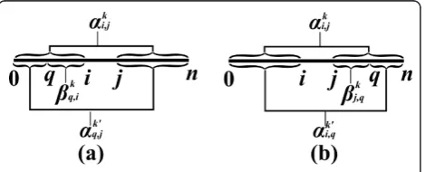
Here, for the case whereμki,j=⊕q∈[0,i)
βk q,i⊗αk
q,j
, the
valueμki,jreflects an expression which examines all pos-sible splits of si,j into a sub-instance of the form sq,j, whereq < i, and a sub-instance of the formsq,i(Figure 10a). Each split induces a term which is obtained by applying the⊗operation between a propertyβqk,iofsq,i and a propertyαkq,jofsq,j. Then,μki,jcombines the values of all such terms by applying the⊕operator.
Symmetri-cally, whenμki,j=⊕q∈(j,n]
αk i,q⊗βjk,q
,μki,jreflects a value
corresponding to the examination of all splits ofsi,jinto a sub-instance of the formsi,q, where q > j, and a sub-instance of the formsj,q(Figure 10b).
We now turn to describe a generic recursive algorithm for Outside VMT problems. For simplicity, we consider the case of a problem whose goal is to compute a single set of outside propertiesa, given a single pre-computed set of inside propertiesb. As for the Inside VMT algo-rithm, it is simple to extend the presented algorithm to the case where the goal is to compute a series of outside properties for every sub-instance of the input.
For an input string sof lengthn, the algorithm main-tains a matrix Aof size ||s|| × ||s||, corresponding to the required output matrix a. In order to compute a propertyai,j, the availability of values of the formai’,j’,
such thatsi,j is a strict substring ofsi’,j’, is required. In terms of the matrixA, this means that when computing Ai, j, all entries in the sub-matrixA[0,i], [j,n], excluding the entryAi, jitself, need to be computed (Figure 11a).
At each recursive call, the algorithm computes the values in a sub-matrix ofA. The following pre-condition is maintained when the algorithm is called over a sub-matrixAI, J(Figure 12):
1. Each entry Ai, jinA[0,I], [J,n]contains the valueai, j, except for entries inAI,J.
2. If the computation of ai, jrequires the result of a vector multiplication of the formμi, j =⊕qÎ[0,i)(bq, i
⊗ aq, j), thenAI, J = (b[0,I),I)T ⊗a[0,I),J. Else, if the computation of ai, j requires the result of a vector multiplication of the form μi,j =⊕qÎ(j,n](ai, q⊗bj,
q), thenAI, J=aI, (j, n]⊗(bj(J,n])T.
The pre-condition implies that whenI= [i, i] andJ= [j, j], all necessary values for computingai, jin o(||s||) running time are available, and thus ai, j can be effi-ciently computed and stored inAi,j. When |I|>1 or |J|
>1, the algorithm follows a similar strategy as that of the Inside VMT algorithm, by partitioning the matrix into two parts, and computing each part recursively. The vertical and horizontal partitions are illustrated in Figure 13 and 14, respectively. The pseudo-code for the complete Outside VMT algorithm is given in Table 3. Similar running time analysis as that applied in the case of the Inside VMT algorithm can be shown, yielding the result stated in Theorem 2.
Theorem 2For every Outside VMT problem there is
an algorithm whose running time over an instance s is
o (||s||3). When the problem sustains the standard VMT settings, the running time of the algorithm is
Θ(M(||s||)), where M(n)is the running time of the cor-responding matrix multiplication algorithm over two n ×n matrices.
5 Multiple String VMT
In this section we describe another extension to the VMT framework, intended for problems for which the instance is a set of strings, rather than a single string.
Examples of such problems are the RNA Simultaneous
Alignment and Folding problem [15,37], which is
described in details in Appendix B, and the RNA-RNA
Interaction problem [9]. Additional problems which
exhibit a slight divergence from the presented template,
such as the RNA-RNA Interaction Partition Function
problem [12] and the RNA Sequence to
Structured-Sequence Alignmentproblem [13], can be solved in simi-lar manners.
In order to define the Multiple String VMT variant in a general manner, we first give some related notation.
Aninstanceof a Multiple String VMT problem is a set
of strings S = (s0, s1, ..., sm-1), where the length of a stringspÎS is denoted bynp. ApositioninSis a set of indicesX = (i0,i1, ..., im-1), where each index ipÎ X is in the range 0≤ip≤np. The number of different posi-tions inSis denoted by||S|| =
0≤p<m||
sp|| .
LetX = (i0,i1, ...,im-1) andY= (j0,j1, ...,jm-1) be two positions inS. Say thatX ≤Yifip≤jpfor every 0≤ p <
m, and say that X < YifX ≤YandX ≠Y. WhenX ≤Y,
denote by SX, Y the sub-instance
SX,Y=
s0
i0,j0, s1i1,j1, . . ., s m−1 im−1,jm−1
of S (see Figure 15a).
Figure 11The base case of the Outside VMT algorithm. (a) An illustration of the matrixAupon computingAi,j. (b) An illustration
of the pre-computed matrixb. All required values of the formai’,j’
for computingai,jhave already been computed in the sub-matrix A[0,i], [j,n], excluding the entryAi,jitself.μi,jis obtained either by the multiplication (b[0,i),i)
T
⊗A[0,i),j(the multiplication of the transposed striped dark gray vector inbwith the striped dark gray vector inA), or by the multiplicationAi,(j, n]⊗(bj,(j, n])T(the multiplication of the
non-striped dark gray vector inAwith the transposed non-striped dark gray vector inb).
Figure 12The pre-condition of the Outside VMT algorithm. (a) An illustration of the matrixAupon computingAI,J(dotted entries). (b) An illustration of the pre-computed matrixb. The pre-condition requires that all entries in the sub-matrixA[0,I], [J,n], excludingAI,J, are
computed (dark and light gray entries). In addition,AI,Jis either the result of the matrix multiplication (b[0,I),I)T⊗a[0,I),J(the
multiplication of the transposed striped dark gray matrix inbwith the striped dark gray matrix inA), or the multiplicationaI,(J, n]⊗(bJ,
(J,n])
T
Say thatSX’, Y’is astrict sub-instance ofSX,YifX≤X’≤
Y’≤Y, and SX’,Y’≠SX,Y.
The notation X ≰Yis used to indicate that it is not true that X ≤ Y. Here, the relation ‘≤’ is not a linear relation, thusX ≰Ydoes not necessarily imply thatY < X. In the case whereX ≰Y, we say thatSX, Ydoes not correspond to a valid sub-instance (Figure 15b). The notations0¯ andN will be used in order to denote the first position (0, 0, ..., 0) and the last position (n0,n1, ...,
nm-1) in S, respectively. The notations which were used previously for intervals, are extended as follows: [X, Y] denotes the set of all positionsQ such thatX ≤Q≤ Y, (X,Y) denotes thesetof all positionsQsuch thatX < Q
< Y, [X,Y) denotes thesetof all positionsQsuch thatX
≤ Q < Y, and (X, Y] denotes the set of all positions Q such that X < Q≤ Y. Note that while previously these notations referred to intervals with sequential order defined over their elements, now the notations corre-spond to sets, where we assume that the order of ele-ments in a set is unspecified.
Inside and outside properties with respect to multiple string instances are defined in a similar way as for a sin-gle string: An inside property bX, Y is a property that depends only on the sub-instance SX, Y, where an out-side propertyaX, Ydepends on the residual sub-instance
of S, after excluding from each string in S the
Figure 13The vertical decomposition in the Outside VMT algorithm, for the case where |I|≤|J|. (a)AI,Jsustains the pre-condition (see Figure 12 for notations). (b)AI,Jis partitioned vertically toAI,J1andAI,J2, whereAI,J1is computed recursively. (c) Ifμi,jis of the form⊕qÎ(j,n]
(ai,q⊗bj,q), then the pre-condition for computingAI,J2is established, by updatingAI,J2to be
AI,L⊗(βJ2,L)T
⊕AI,J2(in this exampleL =J1, sinceIends beforeJ1starts. The corresponding sub-matrix ofbis not shown). In the case whereμi,j=⊕qÎ[0,i)(bq,i⊗aq,j), the
pre-condition is met without any need for performing a matrix multiplication. Then,AI,J2is computed recursively (not shown).
Figure 14The horizontal decomposition in the Outside VMT algorithm, for the case where |I|>|J|. (a)AI,Jsustains the pre-condition (see Figure 12 for notations). (b)AI,Jis partitioned horizontally toAI1,JandAI2,J, whereAI1,Jis computed recursively. (c) Ifμi,jis of the form⊕qÎ[0,
i)(bq,i⊗aq,j), then the pre-condition for computingAI2,Jis established, by updatingAI2,Jto beAI2,J⊕
(βL,I2)T⊗AL,J
(in this example L=I1, sinceI2ends beforeJstarts. The corresponding sub-matrix ofbis not shown). In the case whereμi,j=⊕qÎ(j,n](ai,q⊗bj,q), the
corresponding substring in SX, Y. In what follows, we defineMultiple String Inside VMTproblems, and show how to adopt the Inside VMT algorithm for such pro-blems. The “outside” variant can be formulated and solved in a similar manner.
Definition 3 A problem is considered a Multiple
String Inside VMT problem if it fulfills the following requirements.
1. Instances of the problem are sets of strings, and the goal of the problem is to compute for every sub-instance SX, Y of an input instance S, a series of
inside propertiesβX1,Y, β2
X,Y, . . ., βXK,Y.
2. Let SX, Ybe a sub-instance of some input instance
S. Let1 ≤k ≤K, and letμk
X,Ybe a value of the form
μk
X,Y=⊕Q∈(X,Y)
βk X,Q⊗βk
Q,Y
, for some 1 ≤ k’, k” ≤ K. Assume that the following values are available:
μk
X,Y,all valuesβk
X,Yfor 1≤k’≤K and SX’,Y’a strict
sub-instance of SX, Y, and all valuesβk
X,Yfor1 ≤k’< k. Then,βk
X,Ycan be computed in o (||S||)running time.
3. In the multiplication variant that is used for com-putingμk
X,Y, the⊕operation is associative and com-mutative, and the domain of elements contains a zero element. In addition, there is a matrix multipli-cation algorithm for this multiplimultipli-cation variant,
which running time M(n) over two n × n matrices
satisfies M(n) =o(n3).
Note that here there is an additional requirement with respect to the single string variant, that the⊕operator
is commutative. This requirement was added, since
while in the single string variant split positions in the interval (i,j) could have been examined in a sequential order, and the (single string) Inside VMT algorithm retains this order when evaluatingμki,j, here there is no such natural sequential order defined over the positions in the set (X, Y). The⊕commutativity requirement is met in all standard variants of matrix multiplication, and thus does not pose a significant restriction in practice.
Consider an instanceS= (s0,s1, ...,sm-1) for a Multiple String Inside VMT problem, and the simple case where a single property setbneeds to be computed (where b corresponds to all inside properties of the formbX, Y). Again, we compute the elements ofbin a square matrix
Table 3 The outside VMT algorithm
Outside-VMT(s,b)
1: Allocate a matrixAof size ||s|| × ||s||, and initialize all entries in Awithjelements.
2: CallCompute-Outside-Sub-Matrix([0,n], [0,n]), where nis the length ofs.
3: returnA
Compute-Outside-Sub-Matrix(I,J)
pre-condition:The values inA[0,I], [J,n], excluding the values inAI,J, are
computed.
Ifμi,j=⊕qÎ[0,i)(bq,i⊗aq,j), thenAI,J= (b[0,I),I)T⊗a[0,I),J. Else, ifμi,j=
⊕qÎ(j,n](ai,q⊗bj,q), thenAI,J=aI,(J,n]⊗(bJ,(J,n])
T .
post-condition:A[0,I], [J,n]=a[0,I], [J,n].
1: ifI= [i,i] andJ= [j,j]then
2: Ifi≤j, computeai,j(ino(||s||) running time) by querying computed values inAand the valueμi,jwhich is stored inAi,j. UpdateAi,j¬ai,j.
3: else
4: if|I|≤|J|then
5: LetJ1andJ2be the two intervals such thatJ2J1=J, and | J2| =⌊|J|/2⌋.
6: CallCompute-Outside-Sub-Matrix(I,J1).
7: ifμi,jis of the form⊕qÎ(j,n](ai,q⊗bj,q)then 8: LetLbe the interval such thatL(J,n] = (J2,n].
9: UpdateAI,J2 ←
AI,L⊗(βJ2,L)T
⊕AI,J2. 10: end if
11: CallCompute-Outside-Sub-Matrix(I,J2).
12: else
13: LetI1andI2be the two intervals such thatI1I2=I, and | I1| =⌊|I|/2⌋.
14: CallCompute-Outside-Sub-Matrix(I1,J).
15: ifμi,jis of the form⊕qÎ[0,i)(bq,i⊗aq,j)then 16: LetLbe the interval such that [0,I)L= [0,I2).
17: UpdateAI2,J←AI2,J⊕
(βL,I2)T⊗AL,J
. 18: end if
19: CallCompute-Outside-Sub-Matrix(I2,J).
20: end if
21: end if
Figure 15Multiple String VMT. (a) An example of a Multiple String VMT instance, with three strings. A sub-instanceSX,Yconsists of three substrings (whereX= {i0,i1,i2} andY= {j0,j1,j2}). (b) Here, sincej1< i1we have thatX≰Y, and thusSX,Ydoes not correspond to a valid sub-instance. (c) A valid split of the sub-instance is obtained by splitting each one of the corresponding substringsspip,jpinto a prefixspip,qpand a suffixspq
Bof size ||S|| × ||S||, and show that values of the form
μX, Ycorrespond to results of vector multiplications within this matrix. For simplicity, assume that all string spÎSare of the same lengthn, and thus ||S|| = (n+ 1) m
(this assumption may be easily relaxed).
Define a one-to-one and onto mapping h between
positions in S and indices in the interval [0, ||S||), where for a positionX = (i0, i1, ...,im-1) inS,
h(X) =mp=0−1ip·(n+ 1)p. Let h-1 denote the inverse mapping ofh, i.e. h(X) = i⇔h-1(i) =X. Observe thatX
≤Yimplies that h(X)≤h(Y), though the opposite is not necessary true (i.e. it is possible that i≤ jand yeth-1(i)
≰h-1(j), as in the example in Figure 15b).
Each value of the form bX, Y will be computed and
stored in a corresponding entryBi, j, wherei=h(X) and
j=h(Y). Entries ofB which do not correspond to valid sub-instances ofS, i.e. entriesBi,jsuch that h-1(i)≰h-1 (j), will hold the value j. The matrixB is computed by applying the Inside VMT algorithm (Table 2) with a simple modification: in the base-cases of the recurrence (line 2 in Procedure Compute-Inside-Sub-Matrix, Table 2), the condition for computing the entry Bi,jis thath-1 (i)≤h-1(j) rather thani≤j. Ifh-1(i)≤h-1(j), the property βh−1(i),h−1(j)is computed and stored in this entry, and otherwise the entry retains its initial valuej.
In order to prove the correctness of the algorithm, we only need to show that all necessary values for comput-ing a propertybX, Yare available to the algorithm when the base-case of computing Bi, j fori =h(X) and j=h (Y) is reached. Due to the nature of the mapping h, all propertiesbX’,Y’for strict sub-instancesSX’,Y’ofSX, Y cor-respond to entriesBi’,j’such thati’=h(X’) andj’=h(Y’)
andi’,j’Î [i,j]. Therefore, all inside properties of strict sub-instances ofSX,Yare available according to the pre-condition. In addition, at this stage Bi, j contains the value Bi,(i,j)×B(i,j),j. Note that for every QÎ (X, Y), q=
h(Q)Î (i,j) (Figure 16a), and thus bX,Q ⊗bQ,Y=Bi,q
⊗Bq,j. On the other hand, everyq Î (i,j) such that Q =h-1(q) ∉(X, Y) sustains that either X ≰Q orQ ≰Y (Figure 16b), and therefore eitherBi, q =jorBq, j=j, and Bi, q ⊗Bq, j= j. Thus,Bi, (i, j) ×B(i,j),j =⊕QÎ(X,Y) (bX, Q ⊗bQ, Y) = μX, Y, and according to the Multiple
String VMT requirements, the algorithm can compute
bX,Yino(||S||) running time.
The following theorem summarizes the main result of this section.
Theorem 3For every Multiple String (Inside or
Out-side) VMT problem there is an algorithm whose running time over an instance S is o (||S||3). When the problem sustains the standard VMT settings, the running time of the algorithm isΘ(M(||S||)), where M(n)is the running time of the corresponding matrix multiplication algo-rithm over two n×n matrices.
6 Concluding remarks
This paper presents a simplification and a generalization of Valiant’s technique, which speeds up a family of algo-rithms by incorporating fast matrix multiplication pro-cedures. We suggest generic templates that identify problems for which the approach is applicable, where these templates are based on general recursive proper-ties of the problems, rather than on their specific algo-rithms. Generic algorithms are described for solving all problems sustaining these templates.
The presented framework yields new worst case run-ning time bounds for a family of important problems. The examples given here come from the fields of RNA secondary structure prediction and CFG Parsing. Recently, we have shown that this technique also applies for the Edit Distance with Duplication and Contraction problem [45], suggesting that it is possible that more problems from other domains can be similarly acceler-ated. While previous works describe other practical acceleration techniques for some of the mentioned pro-blems [14,25,28,32-38], Valiant’s technique, along with the Four Russians technique [28,30,31], are the only two techniques which currently allow to reduce the theoreti-cal asymptotic worst case running times of the standard algorithms, without compromising the correctness of the computations.
The usage of the Four Russians technique can be viewed as a special case of using Valiant’s technique. Essentially, the Four Russians technique enumerates solutions for small computations, stores these solutions
Figure 16Thehmapping. The notationsX,Y, andQ, refer to the positions (i1,i2,i3), (j1,j2,j3) and (q1,q2,q3) which are illustrated in the figure,
respectively. (a) A positionQÎ(X,Y) is mapped to an indexqÎ(i,j), wherei=h(X) andj=h(Y). (b) Some indicesqÎ(i,j) correspond to positionsQ=h-1(q) such thatQ