M E T H O D O L O G Y
Open Access
Cluster ensemble based on Random
Forests for genetic data
Luluah Alhusain
*and Alaaeldin M. Hafez
* Correspondence: [email protected] College of Computer and Information Sciences, King Saud University, Riyadh, Saudi Arabia
Abstract
Background:Clustering plays a crucial role in several application domains, such as bioinformatics. In bioinformatics, clustering has been extensively used as an approach for detecting interesting patterns in genetic data. One application is population structure analysis, which aims to group individuals into subpopulations based on shared genetic variations, such as single nucleotide polymorphisms. Advances in DNA sequencing technology have facilitated the obtainment of genetic datasets with exceptional sizes. Genetic data usually contain hundreds of thousands of genetic markers genotyped for thousands of individuals, making an efficient means for handling such data desirable.
Results:Random Forests (RFs) has emerged as an efficient algorithm capable of handling high-dimensional data. RFs provides a proximity measure that can capture different levels of co-occurring relationships between variables. RFs has been widely considered a supervised learning method, although it can be converted into an unsupervised learning method. Therefore, RF-derived proximity measure combined with a clustering technique may be well suited for determining the underlying structure of unlabeled data. This paper proposes, RFcluE, a cluster ensemble approach for determining the underlying structure of genetic data based on RFs. The approach comprises a cluster ensemble framework to combine multiple runs of RF clustering. Experiments were conducted on high-dimensional, real genetic dataset to evaluate the
proposed approach. The experiments included an examination of the impact of parameter changes, comparing RFcluE performance against other clustering methods, and an assessment of the relationship between the diversity and quality of the ensemble and its effect on RFcluE performance.
Conclusions:This paper proposes, RFcluE, a cluster ensemble approach based on RF clustering to address the problem of population structure analysis and demonstrate the effectiveness of the approach. The paper also illustrates that applying a cluster ensemble approach, combining multiple RF clusterings, produces more robust and higher-quality results as a consequence of feeding the ensemble with diverse views of high-dimensional genetic data obtained through bagging and random subspace, the two key features of the RF algorithm.
Keywords: Cluster ensemble, Random Forests, Genetic population, Population structure analysis, Random Forest proximity, High-dimensional data, Ensemble diversity, Single nucleotide polymorphism, Normalized mutual information
Background
Clustering is an unsupervised learning technique aimed at uncovering the underlying natural structure of data. In data analysis, clustering is the process of partitioning objects into groups based on their similarities, where objects in the same group are more similar to one another than to objects in different groups. Clustering plays an essential role in several application domains, such as text mining, image segmentation, and bioinformatics. In bioinformatics, clustering has been extensively used as an approach for detecting interesting patterns in gen-etic data. Such an approach is formally used to find the underlying population substructure from genetic data without considering prior information. The analysis of population structures is a crucial prerequisite for any further analysis of genetic data, such as genome-wide associ-ation mapping [1] for reducing false positive rates, and forensics [2] for developing reference panels to provide information on an individual’s ancestry. This kind of analysis aims to group individuals into subpopulations based on shared genetic variations. Single nucleotide polymor-phisms (SNPs) are the most common type of genetic variation used to infer population struc-ture. SNPs occur when a single nucleotide from a DNA sequence differs at the same position between individuals. An SNP has three categories: homozygous with the common allele (genotype AA), heterozygous (genotype AB), and homozygous with the rare allele (genotype BB). Advances in DNA sequencing technology have facilitated the attainment of genetic data-sets with exceptional sizes. Genetic data usually contain hundreds of thousands of genetic markers genotyped for thousands of individuals. Thus, an efficient means for handling such high-dimensional data is desirable.
Two major clustering approaches have been developed to infer the structure of populations from genetic data: distance-based and dimension reduction-based ap-proaches. AWclust [3] is a distance-based approach that consists of constructing an allele-sharing distance (ASD) matrix between all pairs of individuals in the gen-etic data. It then applies hierarchical clustering to infer clusters of individuals from the ASD matrix using Ward’s algorithm. PCAclust [4] is a dimension reduction-based clustering approach that involves applying principal component analysis (PCA) to reduce the dimensions of the genetic data. It then applies a model-based clustering algorithm (i.e., a Gaussian mixture model clustering) to the set of rele-vant principal components.
RF clustering, in which RF-derived proximity is combined with a clustering tech-nique, is well suited for discovering the underlying structure of unlabeled data [6, 7]. However, the main concern underlying the RF algorithm is that, for each run, a different proximity matrix is generated due to its random nature, therefore produ-cing a different clustering result each time. Thus, this paper proposes a Random Forest cluster Ensemble (RFcluE) approach to discover the underlying structure of genetic data. Within this approach, a cluster ensemble framework is utilized to combine the results of multiple runs of RF clustering toward obtaining a more reli-able and robust clustering result than a single run of RF clustering.
Methods
Random Forests
Random Forests (RFs) has emerged as an efficient algorithm capable of handling high-dimensional data [8]. RFs was formally developed by Leo Breiman [8] as a classification and regression ensemble learning method. This method is based on a combination of bagging [9] and random subspace [10]. Baggingis the process of aggregating the results of multiple trees, where each tree is grown on a bootstrap sample of the objects. A bootstrap sample of a specified size is drawn with replacement from the original data. Random subspace refers to the selection of a random subset of variables as candidates for splitting at each node. Rather than considering all variables as candidates for split-ting, RFs considers only a subset of variables, thus reducing the correlation between trees.
In the context of population structure analysis, individuals are the objects, while SNP markers are the variables. Thus, in RFs, a forest is constructed by building multiple de-cision trees. To build a tree, the algorithm first creates a root node containing a boot-strap sample of the individuals. Then, at each node, the algorithm selects a random subset of the markers to search over, and subsequently determines the best split markers based on a splitting criterion. A splitting criterion usually maximizes some measure of node purity, which means the degree to which individuals of a node belong to one class. In RFs, the Gini index [11] is used as a splitting criterion to select the best split at each node. The Gini index measures how well a potential split of a node is in separating the individuals into two known classes. Consequently, the Gini index at nodenis defined as:
Gini nð Þ ¼X C
c¼1
^
pnc1 − p^nc ð1Þ
where p^nc ¼nc
n is the proportion of individuals that are of classc at node n. The Gini
index is minimized when all individuals in the node are of the same class, increasing as the individuals in the node are spread more evenly among different classes. The gain for splitting node n based on markerxi, Gain (xi,n), is defined as the difference be-tween the impurity at nodenand the weighted average of impurities at each child node ofn. That is,
Gain xð i;nÞ ¼Gini xð i;nÞ−wLGini xi;nL
−wRGini xi;nR
andwRare the proportions of individuals assigned to the left and right child nodes. Based on the gain value, the markerxiwith the lowest impurity is selected to split individuals at noden.
This process of splitting is repeated until an unpruned tree is formed. The generated forest contains a significant amount of information about the relationship between the markers and the individuals that can be used for prediction, variable importance, prox-imity calculation, missing data imputation, and outlier detection. RF-derived proxprox-imity, a byproduct of a random forest, is defined based on similar individuals ending up in the same leaf node more often than dissimilar individuals. This proximity can capture different levels of co-occurring relationships between markers.
RFs is widely considered a supervised learning method, although it can be adapted as an unsupervised learning method to derive proximity matrix from unlabeled data [6]. Recently, unsupervised RFs has been successfully applied in a wide variety of domains, including bioinformatics [6, 12], image and document analysis [13–15], networking [16], cloud computing [17, 18], manufacturing [19], remote sensing [20], and chemo-metrics [21].
To use RFs for unsupervised learning, the RF algorithm must first randomly generate synthetic data based on the original dataset, in which a random forest is built to distin-guish the original data from the synthetic data. One approach for generating the syn-thetic data is to randomly draw synsyn-thetic individuals from marginal distributions of each observed marker in the original data [4]. Hence, the synthetic class has a distribu-tion of independent random markers, where each marker follows the same distribudistribu-tion as the corresponding marker in the original data.
Cluster ensemble
A cluster ensemble is an effective approach for combining different clusterings of the same dataset into a more robust and higher-quality clustering than any individual clus-tering. A cluster ensemble typically consists of two components: an ensemble con-structor and a consensus function. An ensemble concon-structor generates a set of different partitions of the dataset, which is referred to as “base clusterings”or “ensemble mem-bers.” On the other hand, a consensus function combines the base clusterings of the ensemble and produces a single clustering as the ultimate output of the cluster ensemble.
Regarding the ensemble constructor, several methods have been proposed to obtain ensemble members, including applying different clustering algorithms [22, 23], applying the same clustering algorithm with random parameter initializations [24–26], project-ing data onto different subspaces [26–28], and data subsampling [25, 29, 30].
objects, which can be used as an input to any similarity-based clustering to derive the final partition [23, 25, 27, 33, 34].
Cluster ensemble based on Random Forests
The proposed approach, the Random Forest cluster Ensemble (RFcluE), is based on the concept of a cluster ensemble, where RF clustering is used as a base clustering method. The general framework for the RFcluE approach is shown in Fig. 1. The RFcluE ap-proach has two stages: The first stage is ensemble construction, followed by the con-sensus function stage. The first stage takes a genetic dataset as an input and then outputs a set of partitions. The second stage takes the set of partitions as an input and produces a final clustering result as an output.
Let G= {g1,g2,…,gN} represent a set of N individuals, where gi is a genotype pro-file of individual i that consists of l genetic markers. A cluster ensemble first con-structs a set of partitions (i.e., ensemble members), P= {P1,P2,…,PM}, by applying
the base clustering method M times. Each run of the base clustering method
returns a set of clusters, Pi¼ C1i;C2i;…:;C ki
i
n o
;such that ⋃ki
j¼1Cji¼G, where ki is
the number of clusters in the ith clustering and Cji is the jth cluster of the ith parti-tion, for i= 1, 2, …, M. Then, the consensus function is applied to the set of gen-erated partitions, P, in order to find a new partition, P∗, that better represents the properties of each partition in P of the cluster ensemble.
Ensemble construction
The ensemble construction based on RFs is used to create the base clusterings. Cluster-ing usCluster-ing RFs is generally composed of three steps:
(i) Constructing a forest in an unsupervised fashion.
(ii)Parsing the constructed forest to compute the proximities between individuals. (iii)Applying a clustering technique on the resulting proximity matrix.
The input of the ensemble constructor is a genetic dataset, GЄRN×l, whereNis the number of individuals and l is the number of genetic markers; and four parameters, specifically the number of trees (ntrees), the tree size controlled by specifying the max-imum number of leaf nodes (MN), the number of clusters in each partition (k), and the ensemble size (M).
Since the base clustering method of the ensemble is RF clustering, the ensemble constructor first computes the RF-derived proximity matrix. The algorithm that builds a random forest, RF, of size ntrees trees, where each tree has a maximum of MN leaf nodes in the unsupervised mode, is described in Algorithm 1. Based on the constructed forest, the RF-derived proximity matrix, which denotes the similarity between each pair of individuals of size N×N, is calculated. Then, the
proximity matrix S is converted to a dissimilarity matrix, D, by using D¼pffiffiffiffiffiffiffiffiffiffiffið1−sÞ. Lastly, the method applies K-means on this dissimilarity, after transforming it to Euclidean space using multidimensional scaling (MDS) [35], to partition the indi-viduals into k clusters. The MDS technique used is classical scaling, where a N× N distance matrix is converted into a N×p configuration matrix. The configur-ation matrix contains the coordinates of N individuals in p-dimensional space, where p<N; p is determined such that the dimension of the smallest space in which N individuals can be embedded, given D that contains the inter-distances between individuals.
The output of the base clustering, RF clustering, is a single partition of the data. To construct a cluster ensemble of size M partitions, the base clustering method is re-peated M times and, for each run, a different partition of data is generated such that the cluster ensemble isP= {P1,P2,…,PM}. The pseudo-code of the ensemble
Consensus function
Given a cluster ensembleP,Pcontains a set ofMpartitions,P= {P1,P2,…,PM}, produced
by the ensemble construction. Each partition Pi returns a set of clusters such that Pi
¼ C1i;C2i;…:;Cki
i
n o
, wherekiis the number of clusters inPi. Each partitionPicontains
the cluster labels ofNindividuals, such thatc(n) denotes the cluster label to which the in-dividualnbelongs. The goal of the consensus function is to find a new partition,P∗,that combines the information from the cluster ensemble P. The pseudo-code of the consen-sus function of RFcluE is outlined in Algorithm 3. It works as follows. First, the consenconsen-sus function calculates the co-association matrix (CO). CO summarizes the information in the ensemblePas theN×Nmatrix. This matrix denotes the similarity between any pair of N individuals as a proportion of M partitions in the ensemble P, in which they are assigned to the same cluster. Then, the consensus function applies agglomerative hier-archical clustering based on Ward’s minimum variance algorithm [36, 37] on the CO matrix to obtain the final partition,P∗. Ward’s algorithm is utilized because the inference of population structure needs an algorithm that minimizes the increase of within-cluster variance each time an individual is added to a cluster.
Datasets
Evaluation metrics
Many experiments were conducted to investigate the performance of the RFcluE ap-proach. The performance evaluation comprised an assessment of the quality of the final clustering result of the approach. Besides, an assessment of the quality and diversity of the base clusterings, which are generated by the ensemble constructor, was conducted in order to study their impact on performance. Both quality and diversity were evalu-ated based on normalized mutual information (NMI).
NMI is a measure of agreement between two partitions based on information theory [28]. It treats the two partitions as nominal random variables. The NMI score between two partitions, AandB, is computed as:
NMI Að ;BÞ ¼ MI Að ;BÞ H Að Þ þH Bð Þ
ð Þ=2 ð3Þ
MI(A,B) is the mutual information between two partitions, A and B, calculated as follows:
MI Að ;BÞ ¼X
kA
i¼1
XkB
j¼1
Nij
N log NijN
Ni:N:j
ð4Þ
H(A) and H(B) are the entropy of partition A and partition B, respectively, and are calculated as:
H Að Þ ¼−X
kA
i¼1
Ni:
N log Ni:
N ð5Þ
Table 1The description of real genetic datasets
Dataset Number of Individuals Number of SNPs Number of Populations
HapMap 762 46,256 11
Pan-Asian 443 54,794 10
H Bð Þ ¼−X
kB
j¼1
N:j
N log N:j
N ð6Þ
wherekAis the number of clusters in partitionA,kBis the number of clusters in parti-tion B,Niis the number of individuals in clusteri(Ci) of partitionA,Njis the number of individuals in clusterj(Cj) of partitionB, andNijis the number of shared individuals between clusteriof partitionAand clusterjof partitionB(Ci∈AandCj∈B).
Therefore, the NMI score becomes:
NMI Að ;BÞ ¼ − 2PkA
i¼1
PkB
j¼1Nij log NNi:ijNN:j
PkA
i¼1Ni: log NNi: þ
PkB
j¼1N:j log NN:j
ð7Þ
Note that 0≤NMI(A,B)≤1 , so it takes its maximum value if partitionsAandBare identical, and its minimum value if partitionsAandBare independent.
Let P represent a cluster ensemble that contains a set of generated M base parti-tions P= {P1,P2,…,PM}, P∗ is the final clustering result of the cluster ensemble
ap-proach, andLis the truth population labels of individuals.
Based on NMI, the quality of the final clustering result P∗of an ensemblePis calcu-lated as follows:
Q Pð Þ ¼ NMI Pð ;LÞ ð8Þ
The diversity between two partitions, Pi, Pj,is denoted as (1−NMI(Pi,Pj ) ). There-fore, the diversity of an ensemble P is the average of all pairwise diversities among all pairs of partitions—Pi,Pj∈P—and can be calculated as follows:
DS Pð Þ ¼ 2 M Mð −1Þ
X
M−1
i¼1
XM
j¼iþ1
1−NMI Pi; Pj
ð9Þ
where the higher theDS(P) value, the more diverse the ensemble.
The quality of cluster ensemble P is the average quality of all partitions, Pi∈P, and can be calculated as follows:
Q Pð Þ ¼ 1 M
XM
i¼1
NMI Pð i;LÞ ð10Þ
In the comparison study, the adjusted Rand index (ARI) and accuracy (AC) were used, in addition to NMI.
The ARI [42] is a variation of the Rand index [43] that measures how often similar individuals are assigned to the same cluster and dissimilar individuals to different clus-ters. Given two partitions,AandB, the ARI between A and B is calculated as follows:
ARI Að ;BÞ ¼
PkA
i¼1
PkB
j¼1
Nij
2
−
2PkAi¼1 Ni:
2
PkB j¼1
N:j
2
N Nð −1Þ
1 2
PkA i¼1
Ni:
2
þPkB j¼1
N:j
2
− 2PkA
i¼1
Ni:
2
PkB j¼1
N:j
2
N Nð −1Þ
ð11Þ
of individuals in both cluster iof partitionAand clusterjin partitionB;Ni.is the
num-ber of individuals in cluster i of partition A; and N.j is the number of individuals in
cluster jin partition B. Obtaining a higher value of ARI is better, while random parti-tions yield values close to zero.
AC is used to measure the purity of the resulting clusters. To compute AC, each cluster is first assigned to the population label that is most frequent in that cluster. Then, AC is computed by counting the number of correctly assigned individuals and dividing the sum by the total number of individuals,N, as follows:
AC¼X
i¼1
k ðn
i−miÞ
N ð12Þ
where Nis the number of individuals, kis the number of clusters,niis the number of individuals in cluster i, and miis the number of individuals with the majority popula-tion label in clusteri.
Since each run of ensemble clustering would generate different results, all the metrics are reported as an average value of 20 random runs.
Results and discussion
Many experiments were conducted on the real genetic datasets described previously to assess the RFcluE approach in clustering high-dimensional genetic data to infer popula-tion structure, including parameter analysis, consensus funcpopula-tion, comparison study, and diversity and quality analysis.
Parameter analysis
The objective of the parameter analysis was to study the impact of the change in the parameters on RFcluE performance. In this analysis, both the diversity and quality of the ensemble (i.e., base clusterings), in addition to the quality of the final clustering, were considered. Running RFcluE involves the choice of two RF parameters, the num-ber of trees in the forest (ntrees), and the tree size by specifying the maximum number of leaf nodes (MN). In addition to RF parameters, there is the ensemble sizeM, which is the number of times the base clustering method is executed. The last parameter is the number of clusters,k, as an input to the base clustering method. For the consensus function, the only parameter to be specified is the number of clusters for the final clus-tering result. To eliminate its effect in evaluation, the consensus function is forced to divide the individuals into K clusters, where Kis the number of the true populations for the examined datasets. Therefore, the final clustering result can be evaluated against the corresponding truth population labels for the dataset.
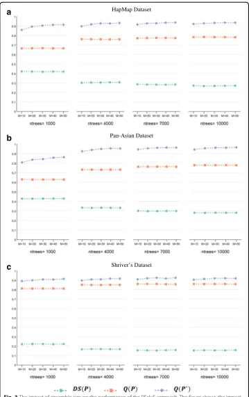
Figure 2 plots the values of the diversity and quality of the ensemble as well as the qual-ity of the ensemble’s final clustering to show the impact of the change in RF parameters. For each dataset, we tested these values (ntrees= {1000, 4000, 7000, 10000}, MN
value of the maximum number of leaf nodes,MN ¼pffiffiffiffiN, is empirically sufficient to con-trol the tree size in the forest. This value is also more efficient as it takes less time to run the RF algorithm. Additionally, the plots show that an increase in the number of trees is associated with a decrease in the diversity and an increase in the quality of the base clus-terings, as well as an increase in the quality of the ensemble’s final clustering. These trends varied for each dataset. For the Pan-Asian dataset, there was a positive correlation be-tween the performance improvement of the ensemble clustering and the number of trees, where a significant improvement was seen when the number of trees increased from 1000 to 4000. For the HapMap dataset, we observed similar, albeit minor, improvements as the number of trees increased. For Shriver’s dataset, the performance gain was negligible as the number of trees increased. From these observations, we can conclude that the number of trees is dataset-dependent and must be sufficient to uncover the structure of the exam-ined dataset.
Figure 3 shows the impact of ensemble size on the performance of ensemble cluster-ing, considering both ensemble size and the number of trees. In this figure, the plots report the values of the diversity and quality of the ensemble as well as the quality of the final clustering, where the parameters are: (M= {10, 20, 30, 40, 50}, ntrees= {1000, 4000, 7000, 10000},MN¼pffiffiffiffiN, andk¼pffiffiffiffiN). In general, we can see that the diversity and quality of the ensemble are similar across the five different ensemble sizes for all datasets. However, the quality of the ensemble’s final clustering improves as the ensem-ble size increases. The improvement in overall performance is dependent on the exam-ined dataset, with the Pan-Asian dataset demonstrating the most significant improvement. We can also see that the impact of the ensemble size parameter is diminished as the number of trees in the forest is increased. On the other hand, for Shriver’s dataset, we can see stable performance despite a change in the number of trees and only slight improvement when increasing the ensemble size.
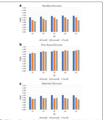
The last parameter is the number of clusters,k, as an input to the base clustering method. In order to study the impact of this parameter, three schemes were defined to determine the number of clusters, namelyTrueK,FixedK, andRandomK. Specifically, letKandNrepresent the number of true clusters and the number of individuals in the examined dataset, respect-ively. The number of clusters for TrueK is k=K; for FixedK, the number of clusters is k
¼pffiffiffiffiN, while forRandomKthe number is random, selected such thatk2;pffiffiffiffiN for each run of the base clustering method. To compare the performance of the three schemes, an ex-periment was conducted using these parameters (M={10, 20, 30, 40, 50},ntrees= 10000,MN
¼pffiffiffiffiffiffiN ). Fig. 4 shows, for each dataset, a bar plot of the NMI values of the three schemes across five ensemble sizes. Regardless of ensemble size, the FixedKscheme had higher NMI than the other two schemes for the HapMap and Shriver datasets. As for the Pan-Asian data-set, no significant difference was observed between the three schemes. This observation thus confirms the performance gain of the ensemble’s final clustering when the number of clusters in base clusterings is overproduced. Likewise, this observation also supports the recommenda-tion that the value ofkbe set to greater than the expected number of clusters [44–46].
Consensus function
b
Pan-Asian Dataseta
HapMap Datasetc
Shriver’s DatasetFig. 2The impact of the change of RF parameters on the performance of the RFcluE approach. The figure shows the impact of the number of trees (ntrees) and the tree size controlled by the maximum number of leaf nodes (MN) on the performance of the RFcluE approach measured using the diversity and quality of the base clusterings along with the quality of the ensemble’s final clustering, where M = 40.aHapMap Dataset.
a
HapMap Datasetb
Pan-Asian Datasetc
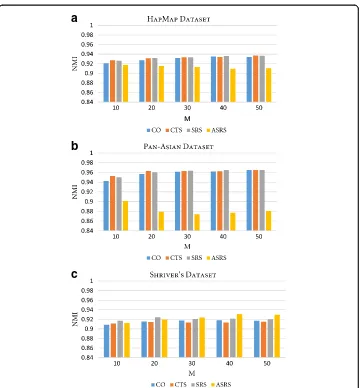
Shriver’s Datasetfunction performs effectively by exploiting the co-association between individuals in the en-semble. However, the ensemble can be explored by considering the association between clus-ters within different partitions in addition to the association between individuals. Link-based similarity measures were proposed in [47] to improve the performance of CO by considering the association between clusters. These measures include connected triple-based similarity (CTS), SimRank-based similarity (SRS) and, finally, the approximate SimRank-based similar-ity (ASRS), which was introduced as an efficient variation of the SRS. Therefore, an experi-ment was conducted to study the impact of these measures on RFcluE performance when utilizing those measures in the consensus function instead of CO. Fig. 5 shows the NMI of applying CO, CTS, SRS, and ASRS to measure the similarity between different partitions of data in the consensus function. The consensus function was applied to the same ensemble,
a
b
c
Fig. 4Performance of three schemes for selecting the number of clusters produced by the base clustering method of RFcluE. The figure shows a plot that compares the performance of three schemes—FixedK, RandomK, and TrueK—for selecting the number of clusters produced by the base clustering method in the RFcluE approach over different ensemble sizes, wherentrees= 10,000 andMN=pffiffiffiN.aHapMap Dataset.bPan-Asian Dataset.
which was generated using this parameter settings (ntrees= 10000, MN¼pffiffiffiffiN, and k
¼pffiffiffiffiN). For all datasets, CO, CTS, and SRS demonstrated comparable performance, while ASRS provided the worst performance compared with other measures for the Pan-Asian data-set. However, ASRS provided the best performance for Shriver’s dataset when the ensemble size was greater than 30. However, the difference in performance between these measures was not statistically significant, with ap-value < 0.05.
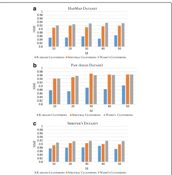
CO used in the consensus function of RFcluE, represents a similarity matrix in which any similarity-based clustering can be applied to obtain the final clustering result. In RFcluE, we applied Ward’s agglomerative hierarchical clustering. However, different clustering techniques can be applied to the CO, such as K-means and spectral clustering. Therefore, another ex-periment was conducted wherein these clustering techniques were applied to the CO to examine their impact on the performance of RFcluE. Fig. 6 shows the NMI of the three clus-tering techniques—Ward’s, K-means, and spectral clustering—when applied to the same ensemble. The parameter settings used for the base clustering method were (M= {10, 20, 30,
a
b
c
40, 50},ntrees= 10000,MN¼pffiffiffiffiN, andk¼pffiffiffiffiN). We can see that Ward’s clustering, ap-plied with RFcluE, has the best performance compared with K-means and spectral clustering across all the examined datasets, demonstrating statistically significant performance, with a p-value < 0.05.
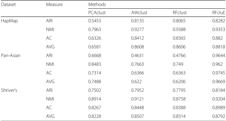
Comparison study
A comparison study was conducted to assess the performance of the proposed ap-proach, RFcluE, against AWclust [48] and PCAclust [4], the two most popular methods for population structure analysis. Moreover, the performance of the RFcluE approach was compared against RFclust. Table 2 and Fig. 7 present the performance of PCAclust, AWclust, RFclust, and RFcluE on the real datasets evaluated using ARI, AC, and NMI. In RFcluE, the clustering result is based on combining multiple runs of RF clustering using a cluster ensemble framework, while RFclust is a clustering method that calcu-lates the average of proximities derived from multiple runs of the RF algorithm and then applies Ward’s agglomerative hierarchical clustering. For RFcluE, the ensemble size M= 40 and FixedK scheme were used. For RFclust, the number of forests was equal to the ensemble size. For both RFcluE and RFclust, the RF parameters were set
a
b
c
such that ntrees= 10000 and MN ¼pffiffiffiffiN. All the compared methods were forced to divide the data into the real number of clusters in the examined dataset. Below, a dis-cussion of the performance of RFcluE, AWclust, and PCAclust is presented, followed by a detailed comparison between RFcluE and RFclust under the same RF parameter settings.
RFcluE, AWclust, and PCAclust
The performance of the RFcluE, AWclust, and PCAclust approaches, based on ARI, AC, and NMI measures, on three real datasets is compared in Table 2. Fig. 7 shows that RFcluE generally outperforms PCAclust and AWclust over the three datasets. The bar plot for the Pan-Asian dataset indicates that RFcluE yields a superior clustering re-sult when compared to the other approaches based on ARI, AC, and NMI. For the HapMap dataset, PCAclust had the worst performance, while RFcluE had the best per-formance. For Shriver’s dataset, all approaches had comparable performance, while RFcluE performed better than the other approaches considering all measures.
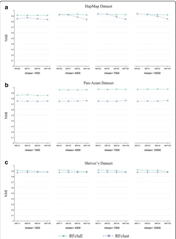
RFcluE versus RFclust
First, the effect of RF parameters was compared for both RFclust and RFcluE. As shown in Fig. 8, when RFclust is used, its performance is in most cases slightly changed as the tree size increases. An exception is HapMap, which shows a slight degradation in per-formance as the tree size increases. This confirms that, like RFcluE, building trees with
MN ¼pffiffiffiffiN is always sufficient for any dataset. On the other hand, RFclust performance was not affected by changing the number of trees per forest nor the number of forests, as shown in Fig. 9. However, its performance was slightly improved with HapMap when in-creasing the number of trees in the forest from 1000 to 4000, and was slightly improved thereafter. Overall, RFclust exhibited stable performance across different values of the number of trees per forest and the number of forests. In addition, small tree sizes are always efficient to provide robust results.
Table 2A performance comparison between PCAclust, AWclust, RFclust, and RFcluE
Dataset Measure Methods
PCAclust AWclust RFclust RFcluE
HapMap ARI 0.5453 0.8135 0.8065 0.8282
NMI 0.7963 0.9277 0.9388 0.9353
AC 0.6326 0.8412 0.8365 0.882
AVG 0.6581 0.8608 0.8606 0.8818
Pan-Asian ARI 0.6668 0.4631 0.4766 0.9644
NMI 0.8483 0.7663 0.749 0.962
AC 0.7314 0.6366 0.6363 0.9745
AVG 0.7488 0.622 0.6206 0.9669
Shriver’s ARI 0.7502 0.7952 0.7795 0.8184
NMI 0.8914 0.9121 0.8758 0.9204
AC 0.8267 0.8448 0.8388 0.8989
AVG 0.8228 0.8507 0.8314 0.8792
The plots in Fig. 8 show that when comparing the performance of RFcluE with that of RFclust under the same RF parameters, RFcluE performs significantly better for all param-eter settings, especially for Pan-Asian datasets. Another paramparam-eter is the number of for-ests to be constructed, which represents the ensemble size within the RFcluE approach. Unlike RFclust performance, RFcluE performance was improved when increasing the number of forests (M), especially when using a smaller number of trees. As shown in Fig. 9, the performance of RFcluE was improved over that of RFclust as the number of trees was increased over different numbers of forests (M). One exception was that RFcluE per-formance for HapMap became similar to that of RFclust when increasing the number of trees from 1000 to 4000, and subsequently stabilized for both approaches. However, the performance of RFcluE was much better than that of RFclust over different numbers of
a
b
c
Fig. 7Performance of PCAclust, AWclust, RFclust, and RFcluE evaluated using ARI, AC, and NMI. The figure shows a plot that compares the performance of PCAclust, AWclust, RFclust, and RFcluE, measured using three measures—ARI, AC, and NMI—along with the average of these measures.aHapMap Dataset.bPan-Asian Dataset.
trees for the Pan-Asian dataset. A similar observation can also be made for Shriver’s data-set, except that the performance of both approaches did not change much across different numbers of trees. This observation indicates that multiple forests with 1000 trees each were enough to discover the structure of Shriver’s dataset.
Overall, we can conclude that it is both crucial and more efficient to use RF cluster-ing as a base clustercluster-ing method within a cluster ensemble framework instead of aver-aging the proximities of several forests and then applying clustering. RFcluE exhibited
a
b
c
Fig. 8The impact of the change of RF parameters on the performance of RFclust vs. RFcluE. The figure shows the impact of the number of trees (ntrees) and the tree size controlled by the maximum number of leaf nodes (MN) om the performance of RFclust and RFcluE measured using NMI.aHapMap Dataset.bPan-Asian Dataset.
better performance than RFclust, especially for clustering in the Pan-Asian dataset. One important observation was that the clustering performance of RFcluE was signifi-cantly improved by increasing the number of forests and the number of trees per forest; unlike RFclust, where these parameters became irrelative. Moreover, the performance of RFcluE was more robust than that of RFclust with respect to tree size as long as suf-ficient trees per forest were constructed.
a
b
c
Fig. 9The impact of the change of the number of forests on the performance of RFclust vs. RFcluE. The figure shows the impact of the number of forests (nforests) on the performance of RFclust and RFcluE, which represents the ensemble size in RFcluE, measured using NMI across different numbers of trees (ntrees).aHapMap Dataset.
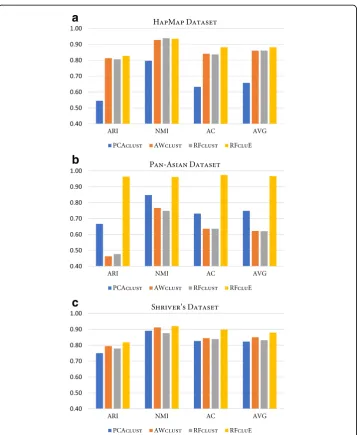
Diversity and quality analysis
The final experiment was conducted to assess the relationship between the diversity and quality of the generated ensemble and its influence on the quality of the ensemble’s final clustering. The diversity of base clusterings is a major factor that could affect the performance of the cluster ensemble approach. On the other hand, the evaluation of the quality of base clusterings is necessary to determine improvements in the quality of the final clustering of the cluster ensemble approach. To perform this experiment, the diversity and quality of base clusterings, as well as the quality of the ensemble’s final clustering, were calculated by applying Eq. (9), Eq. (10), and Eq. (8), respectively.
One source of diversity in base clustering is the number of clusters as an input to the base clustering method.TrueK,FixedK, andRandomKschemes, identified earlier, could generate different levels of diversity among base clusterings. Consequently, an experi-ment was conducted in order to study the diversity and quality of base clusterings
gen-erated by these different schemes with the following parameters: (
M¼40; ntrees¼10000; MN ¼pffiffiffiffiN). Table 3 reports the diversity and quality of base clusterings, as well as the quality of the ensemble’s final clustering over the three datasets. Based on this table, we can observe that the TrueK scheme has the least
Table 4The diversity and quality analysis of the three ensemble-based methods
Dataset Method DS(P) Q(P) Q(P*) Q(P*)-Q(P)
HapMap AWcluE 0.1912 0.8139 0.9148 0.1009
PCAcluE 0.1429 0.7078 0.7510 0.0432
RFcluE 0.2697 0.7823 0.9353 0.1529
Pan-Asian AWcluE 0.1802 0.8356 0.9497 0.1141
PCAcluE 0.0801 0.8427 0.8933 0.0506
RFcluE 0.2800 0.7794 0.9620 0.1826
Shriver’s AWcluE 0.1164 0.8804 0.8879 0.0074
PCAcluE 0.0896 0.8236 0.8351 0.0115
RFcluE 0.1543 0.8592 0.9204 0.0612
The table shows the diversity and quality of the base clusterings (denoted byDS(P) andQ(P), respectively) along with
the quality of the ensemble’s final clustering,Q(P∗), for three datasets using the three ensemble-based clustering
methods: PCAcluE, AWcluE, and RFcluE
Table 3The diversity and quality analysis of the three schemes
Dataset Scheme DS(P) Q(P) Q(P*) Q(P*)-Q(P)
HapMap FixedK 0.2697 0.7823 0.9353 0.1529
RandomK 0.2614 0.7909 0.9208 0.1299
TrueK 0.1542 0.8453 0.9057 0.0604
Pan-Asian FixedK 0.2800 0.7794 0.9620 0.1826
RandomK 0.3204 0.7727 0.9701 0.1974
TrueK 0.1438 0.8799 0.9669 0.0870
Shriver’s FixedK 0.1543 0.8592 0.9204 0.0612
RandomK 0.2555 0.7680 0.8958 0.1279
TrueK 0.1435 0.8530 0.8898 0.0368
The table shows the diversity and quality of the base clusterings (denoted byDS (P)andQ (P), respectively) along with
the quality of the ensemble’s final clustering,Q(P*
), for three datasets using the three different schemes:FixedK,
diversity and the best quality of base clusterings; however, it produces the lowest qual-ity of the ensemble’s final clustering. FixedK produces the highest quality of the final clustering among the three schemes for all datasets. This result confirms that selecting a greater number of clusters for base clustering methods than expected would intro-duce diversity within the ensemble. Thus, higher diversity could lead to more signifi-cant improvement in the quality of the ensemble’s final clustering. To this end, we can conclude that the quality of the base clusterings is not correlated with the quality of the cluster ensemble approach based on RFs, while combining base clusterings could produce a higher-quality final clustering result due to their diversity.
The other sources of diversity are bagging, random subspace, and synthetic data generation applied within unsupervised RF algorithms. Therefore, AWcluE and PCAcluE were developed as an ensemble version of the two single clustering methods, PCAclust and AWclust, to dem-onstrate how the diversity and quality of the base clustering method influence the perform-ance of the entire ensemble, especially RF clustering as a base clustering method of RFcluE. Accordingly, PCAcluE and AWcluE are defined as ensemble-based clustering methods that apply different base clustering methods but utilize the same consensus function of RFcluE. On the one hand, PCAcluE applies PCA and then K-means as a base clustering method. On the other hand, AWcluE calculates ASD and then applies K-means as a base clustering method. For both methods, K-means with a random initialization is considered as a source of diversity that can produce different partitions of the data with varying accuracy.
Table 4 reports the results for each ensemble method over the three datasets using the
same parameters (M= 40,k¼pffiffiffiffiN). By comparing the diversity and quality between the three ensemble-based clustering methods, we can see that RFcluE has the most diverse ensemble across the three datasets with moderate quality. However, it achieves the best performance and exhibits greater improvements in the quality of the ensemble’s final clus-tering over that of base clusclus-terings. From this experimental result, we conjecture that the RF clustering method is most beneficial when applied within a cluster ensemble frame-work. Computing the RF proximity enables viewing high-dimensional genetic data from different angles via bagging and random subspace, thus contributing to a more diverse en-semble than the two other enen-semble-clustering methods. Thus, combining multiple RF clustering results using an ensemble approach produces better clustering result than a sin-gle RF clustering.
Conclusions
indicated that combining multiple clusterings, generated based on RFs, within a cluster ensemble produces high quality and robust clustering results in comparison to a single run of RF clustering. This improvement in performance is a consequence of feeding the ensemble with diverse views of high-dimensional genetic data obtained through bag-ging and random subspace, the two key features of the RF algorithm. To conclude, the major contributions of this paper are proposing and evaluating a cluster ensemble approach based on RFs and demonstrating its effectiveness for high-dimensional, real genetic data. The paper also illustrated that applying a cluster ensemble approach to combine multiple RF clusterings produces more robust and high-quality clustering re-sults than clustering based on averaging the proximities derived from multiple forests. Future work should include the application of the RFcluE approach to other high-dimensional biological data.
Abbreviations
AC:Accuracy; ARI: Adjusted Rand index; ASD: Allele-sharing distance; ASRS: Approximate SimRank-based similarity; CO: Co-association matrix; CTS: Connected-triple-based similarity; LD: Linkage disequilibrium; MDS: Multidimensional scaling; NMI: Normalized mutual information; PCA: Principal component analysis; RFcluE: Random Forest cluster Ensemble; RFclust: Random Forest clustering; SNPs: Single nucleotide polymorphisms; SRS: SimRank-based similarity
Acknowledgements
Not Applicable.
Funding
This research project was supported by a grant from the“Research Center of the Female Scientific and Medical Colleges”, Deanship of Scientific Research, King Saud University.
Availability of data and materials
Pan-Asian dataset is available in the Pan-Asian SNP Consortium website, http://www4a.biotec.or.th/PASNP/, HapMap dataset is available at ftp://ftp.ncbi.nlm.nih.gov/hapmap/phase_3/, and Shriver’s dataset was provided by Prof. Mark D. Shriver.
Authors’contributions
LA designed and implemented the approach, designed and performed the experiments, analyze the results and wrote the manuscript; AH assisted with designing the approach and reviewed the manuscript. All authors read and approved the final manuscript.
Ethics approval and consent to participate
Not applicable.
Consent for publication
Not applicable.
Competing interests
The authors declare that they have no competing interests.
Publisher’s Note
Springer Nature remains neutral with regard to jurisdictional claims in published maps and institutional affiliations.
Received: 27 August 2017 Accepted: 21 November 2017
References
1. Marchini J, Cardon LR, Phillips MS, Donnelly P. The effects of human population structure on large genetic association studies. Nat Genet. 2004;36:512–7.
2. Kidd KK, Pakstis AJ, Speed WC, Grigorenko EL, Kajuna SL, Karoma NJ, Kungulilo S, Kim J-J, Lu R-B, Odunsi A. Developing a SNP panel for forensic identification of individuals. Forensic Sci Int. 2006;164:20–32.
3. Gao X, Starmer J. Human population structure detection via multilocus genotype clustering. BMC Genet. 2007;8:34. 4. Patterson N, Price AL, Reich D. Population structure and eigenanalysis. PLoS Genet. 2006;2:e190.
5. Reich DE, Cargill M, Bolk S, Ireland J, Sabeti PC, Richter DJ, Lavery T, Kouyoumjian R, Farhadian SF, Ward R, Lander ES. Linkage disequilibrium in the human genome. Nature. 2001;411:199–204.
6. Shi T, Horvath S. Unsupervised learning with random Forest predictors. J Comput Graph Stat. 2006;15:118–38. 7. Breiman L, Cutler A. Random forests manual (version 4.0). In Technical Report of the University of California.
9. Breiman L. Bagging predictors. Mach Learn. 1996;24:123–40.
10. Tin Kam H. The random subspace method for constructing decision forests. IEEE Trans Pattern Anal Mach Intell. 1998;20:832–44.
11. Breiman L, Friedman J, Stone CJ, Olshen RA. Classification and regression trees. Wadsworth, New York: Wadsworth Inc.; 1984.
12. Pouyan MB, Birjandtalab J, Nourani M. Distance metric learning using random forest for cytometry data. In: 2016 38th annual international conference of the IEEE engineering in medicine and biology society (EMBC); 16-20 Aug. 2016; 2016. p. 2590. 13. Kumar J, Doermann D. Unsupervised classification of structurally similar document images. In: 2013 12th
International Conference on Document Analysis and Recognition; 25-28 Aug. 2013; 2013. p. 1225–9. 14. Pei Y, Kou L, Zha H. Anatomical structure similarity estimation by random forest. In: 2016 IEEE international
conference on image processing (ICIP); 25-28 Sept. 2016; 2016. p. 2941–5.
15. Du S, Chen S. Detecting co-salient objects in large image sets. IEEE Sig Process Lett. 2015;22:145–8.
16. Wang Y, Xiang Y, Zhang J. Network traffic clustering using random Forest proximities. In: 2013 IEEE international conference on communications (ICC); 9-13 June 2013; 2013. p. 2058–62.
17. Uriarte RB, Tsaftaris S, Tiezzi F. Service clustering for autonomic clouds using random Forest. In: 2015 15th IEEE/ ACM international symposium on cluster, cloud and grid computing; 4-7 may 2015; 2015. p. 515–24. 18. Uriarte RB, Tiezzi F, Tsaftaris SA. Supporting autonomic Management of Clouds: service clustering with random
Forest. IEEE Trans Netw Serv Manag. 2016;13:595–607.
19. Puggini L, Doyle J, McLoone S. Fault detection using random Forest similarity distance. IFAC-PapersOnLine. 2015;48:583–8.
20. Peerbhay KY, Mutanga O, Ismail R. Random forests unsupervised classification: the detection and mapping of <italic>Solanum Mauritianum</italic> infestations in plantation forestry using Hyperspectral data. IEEE J Sel Top Appl Earth Obs Remote Sens. 2015;8:3107–22.
21. Afanador NL, Smolinska A, Tran TN, Blanchet L. Unsupervised random forest: a tutorial with case studies. J Chemom. 2016;30:232–41.
22. Swift S, Tucker A, Vinciotti V, Martin N, Orengo C, Liu X, Kellam P. Consensus clustering and functional interpretation of gene-expression data. Genome Biol. 2004;5:R94.
23. Ayad H, Kamel M. Finding natural clusters using multi-clusterer combiner based on shared nearest neighbors. In Proceedings of the 4th international conference on Multiple classifier systems. Guildford, UK: Springer-Verlag; 2003. p. 166-175.
24. Kim E-Y, Kim S-Y, Ashlock D, Nam D. MULTI-K: accurate classification of microarray subtypes using ensemble k-means clustering. BMC Bioinformatics. 2009;10:260.
25. Monti S, Tamayo P, Mesirov J, Golub T. Consensus clustering: a resampling-based method for class discovery and visualization of gene expression microarray data. Machine Learning. 2003, 52:91-118.
26. Yu Z, Wong H-S, Wang H. Graph-based consensus clustering for class discovery from gene expression data. Bioinformatics. 2007;23:2888–96.
27. Fern XZ, Brodley CE. Random projection for high dimensional data clustering: A cluster ensemble approach. In Proceedings of the 20th International Conference on Machine Learning (ICML-03), Washington, DC, USA. 2003: 186-193. 28. Strehl A, Ghosh J. Cluster ensembles - a knowledge reuse framework for combining multiple partitions. Journal of
Machine Learning Research. 2002;3:583-617.
29. Dudoit S, Fridlyand J. Bagging to improve the accuracy of a clustering procedure. Bioinformatics. 2003;19:1090–9. 30. Minaei-Bidgoli B, Topchy AP, Punch WF. A Comparison of Resampling Methods for Clustering Ensembles. In
Proceedings of the International Conference on Artificial Intelligence; Las Vegas, Nevada, USA. 2004. p. 939-945. 31. Topchy A, Jain AK, Punch W. A mixture model for clustering ensembles. In Proceedings of the 2004 SIAM
International Conference on Data Mining. Lake Buena Vista, Florida: Society for Industrial and Applied Mathematics (SIAM); 2004. p. 379-390.
32. Gionis A, Mannila H, Tsaparas P. Clustering aggregation. ACM Transactions on Knowledge Discovery from Data (TKDD). 2007;1:4.
33. Fred AL, Jain AK. Combining multiple clusterings using evidence accumulation. IEEE Transactions on Pattern Analysis and Machine Intelligence. 2005;27:835-850.
34. Iam-On N, Boongoen T, Garrett S, Price C. New cluster ensemble approach to integrative biological data analysis. International journal of data mining and bioinformatics. 2013;8:150-168.
35. Pekalska E, Duin RPW. The Dissimilarity Representation for Pattern Recognition: Foundations And Applications. Singapore: World Scientific Publishing Co., Inc.; 2005.
36. Ward Jr JH. Hierarchical grouping to optimize an objective function. Journal of the American statistical association 1963;58:236-244.
37. Ward Jr JH, Hook ME. Application of an hierarchial grouping procedure to a problem of grouping profiles. Educational and Psychological Measurement 1963.
38. The International HapMap C. A haplotype map of the human genome. Nature. 2005;437:1299–320.
39. Ngamphiw C, Assawamakin A, Xu S, Shaw PJ, Yang JO, Ghang H, Bhak J, Liu E, Tongsima S, Consortium HP-AS. PanSNPdb: the pan-Asian SNP genotyping database. PLoS One. 2011;6:e21451.
40. Shriver MD, Kennedy GC, Parra EJ. The genomic distribution of human population substructure in four populations using 8525 SNPs. Human Genomics 2004, 1.
41. Shriver MD, Mei R, Parra EJ, Sonpar V, Halder I, Tishkoff SA, Schurr TG, Zhadanov SI, Osipova LP, Brutsaert TD, et al. Large-scale SNP analysis reveals clustered and continuous patterns of human genetic variation. Human Genomics. 2005;2:81.
42. Hubert L, Arabie P. Comparing partitions. Journal of classification. 1985;2:193-218.
43. Rand WM. Objective criteria for the evaluation of clustering methods. Journal of the American Statistical association. 1971;66:846-850.
45. Hadjitodorov ST, Kuncheva LI, Todorova LP. Moderate diversity for better cluster ensembles. Information Fusion. 2006;7:264–75.
46. Kuncheva LI, Hadjitodorov ST. Using diversity in cluster ensembles. In Proceedings of the 2004 IEEE International Conference on Systems, Man, and Cybernetics (ICSMC). The Hague, Netherlands: IEEE; 2004. p. 1214-1219. 47. Iam-on N, Garrett S. LinkCluE: A MATLAB Package for Link-Based Cluster Ensembles. Journal of Statistical Software.
2010.36:9
48. Gao X, Starmer JD. AWclust: point-and-click software for non-parametric population structure analysis. BMC Bioinformatics. 2008;9:77.
• We accept pre-submission inquiries
• Our selector tool helps you to find the most relevant journal • We provide round the clock customer support
• Convenient online submission • Thorough peer review
• Inclusion in PubMed and all major indexing services • Maximum visibility for your research
Submit your manuscript at www.biomedcentral.com/submit