1333
Design And Simulation Of Path Planning
Algorithm For Autonomous Mobile Robot
Navigation System Using EKFSLAM
Kanchustambham Pallav, Gadamsetty Venkata Sai Siva Prasanth, Telaprolu P B M Shanmukha Sree Charan, Deepak Kumar Nayak, Selvakumar. R
Abstract: In the present generation, surroundings molding has become a primary task in the navigation of mobile robots. It is very important for an autonomous robot to automatically build an abstract over surroundings as it is not possible for human intervention all the time. A robot must work on both the localization and mapping to adapt itself to the surroundings. In this work, a surrounding molded algorithm has been developed which purely based on the Extended Kalman Filter (EKF). The mapping and localization issue, called Simultaneous Localization and Mapping (SLAM), is an operation of developing an abstract map on the surroundings to identify the robot coordinates. The SLAM algorithm mainly begins with a mobile robot in an undetermined position without previous knowledge of the surroundings on the map.
Index Terms: Extended Kalman Filter, Simultaneous Localization and Mapping, Mobile Robot Navigation, Path Planning. —————————— ——————————
1
INTRODUCTION
SLAM is an operation, employing an independent robot or an autonomous vehicle, develop or construct a path or track for its climatic or environmental conditions on an uncertain or unclear region on land [1]. At the same time, the autonomous vehicle limits its path or range of area by using the data retrieved before through the route map. At the end of the day, the self-sufficient vehicle attempts to do both mapping and limitation of its track or path simultaneously [4],[6]. The EKF SLAM approach to slam is to develop a filtering process for the system [7]. Our work operates on the two-dimensional SLAM in a three-dimensional environment [3]. It adds the carrying believe of having obstacles or having landmarks that are present in the ground plane. The system is modelled in a discrete-time system, with a variable state denoted by a vector known as state vector. The variables in the state vector can change over the motion of the vehicle, hence the system is dynamic. The EKF-SLAM system is like the estimation of a linear dynamic system.
2
RELATED WORK
The outcome of this work is an understanding of the need for reliable change in maps. Understanding several papers led to the practical implementation of autonomous mapping [8].
It was showed that a mobile robot moves through an unknown environment by knowing relative positions of landmarks, all these estimated landmarks are correlated due to error in estimated vehicle location [9],[10]. This states that a solution to the SLAM problem would require a continuous update of a joint state composed of the vehicle position and every landmark location, with each new landmark. These initial works did not consider the convergence properties of the map in steady state behavior. These map errors were assumed to be growing without bounds rather than converging. This introduced the convergence between Kalman-Filtered based SLAM and reliable methods for mapping and localization. The EKF based SLAM, which has been used in the work is the best way to approach for map building. The importance of this model compared to Kalman-Filter is the ability to represent the non-linear models.
3
PROPOSED WORK
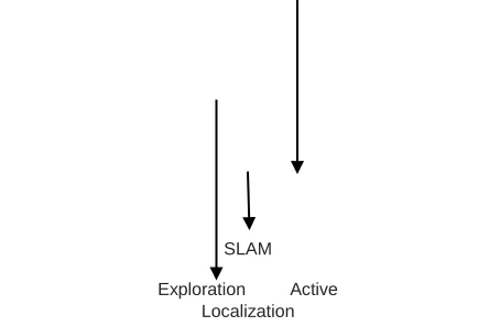
In general, making decisions by the autonomous vehicles in an unknown or unreal situation requires a collective decision of three subtasks, which are mapping, localization, and motion control. Mapping is the operation of inculcating the route map obtained by the vehicle sensors into a given section or region for further process. Ultimately, the movement of an autonomous vehicle is subjected to steer itself in a known path or along an estimated path. The chart in Fig. 1 describes the ————————————————
Kanchustambham Pallav is Final year B.Tech, in electronics & communication engineering in Koneru Lakshmaiah Education Foundation, Vaddeswaram Guntur District, India. E-mail: [email protected]
Gadamsetty Venkata Sai Siva Prasanth is Final year B.Tech, in
electronics & communication engineering in Koneru Lakshmaiah Education Foundation, Vaddeswaram Guntur District, India. E-mail: [email protected]
Telaprolu P B M Shanmukha Sree Charan is Final year B.Tech,
electronics & communication engineering in Koneru Lakshmaiah Education Foundation, Vaddeswaram Guntur District, India. E-mail: [email protected]
Deepak Kumar Nayak Associate Professor, Dept.of ECE,
Koneru Lakshmaiah Education Foundation, Vaddeswaram Guntur District, India.
E-mail: [email protected]
Selvakumar.R Assistant Professor, Dept.of ECE, Koneru
Lakshmaiah Education Foundation, Vaddeswaram Guntur District, India.
E-mail: [email protected]
SLAM
Exploration Active Localization
1334 regions and common regions of these three subtasks. SLAM
has a problem of updating the coordinates in present state where continuous localization helps to overcome the problem by updating the present coordinates.
3.1 Localization
Localization is the process of making an independent robot or autonomous vehicle adaptable to the route or map in that environmental conditions by updating its coordinates continuously. For this continuous updating, we have gone with Relative Filter which is used to compare its current state position with a previous state position. There is no need for connection between landmarks in Relative Filter making it quicker than different techniques.
From the Fig. 2, an independent robot or autonomous vehicle gets the coordinates of two landmarks with the distance of separation. By the coordinates received and the distance of separation it tries to calculate its position. By these assumptions, we can calculate the estimated positions of landmarks for the motion of a robot or vehicle. While Kalman Filter is used to adjust the estimated positions and identify the true positions of landmarks as appeared in Fig.3.
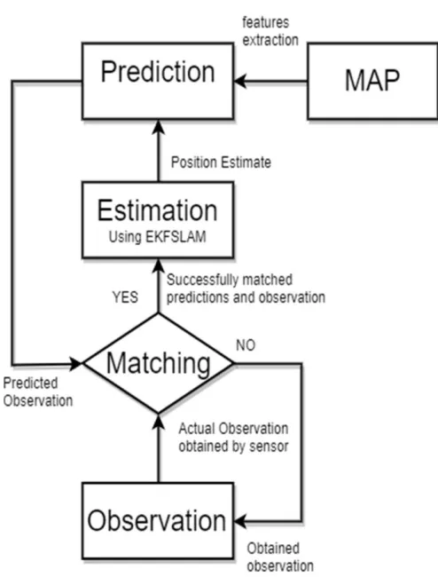
3.2 Flow Chart
4
EKF-SLAM MODEL
Our system uses an Extended Kalman Filter based SLAM which is an extension of the Kalman filter. The Kalman filter deals with only linear systems. However, most navigational problems as the SLAM problem, have non-linear models which renders the direct usage of a Kalman filter not possible. Numerous methods are used to deal with the non-linearity in different SLAM algorithms. An Extended Kalman Filter, one of the more popular methods for handling non-linearity, expects the system models to be differentiable and linearizes the non-linear functions around the current estimates. The SLAM algorithm differs from the Kalman and Extended Kalman filtering algorithms using a joint state that also includes observations.
4.1 The State Vector
The SLAM algorithm utilizes a single joint vector random variable consisting of both the position estimate of the robot and the feature estimates. The robot traverses through the environment, all the while sensing features that are visible and discernible. The state vector, is hence, not of a constant size. Rather, the size of the state vector keeps incrementing with the observation of new features that do not match with previously seen features. The state of the system at time k will be represented by the state vector x(k), consisting of vn scalar random variables for the robot position estimate, and fn vector random variables, each of the fn variables representing the position estimate of one unique feature
Fig. 2: Robot observing landmarks
Fig. 4: low Chart Of EKF-SLAM
1335 where all the coordinates xi,k in the state are denoted relative to
the global frame of reference. The cumulative state vector can be also be expressed by dividing it into two parts, the robot position vector and the feature vector:
where xv,k is the robot position vector and xm,k is the map vector, the vector of all features in the map. The robot is considered an Autonomous Ground Vehicle (AGV), so it travels only in the two-dimensional plane, and its location can be represented using two scalars. However, the robot also possesses a heading which also needs to be represented in the robot position. Thus,
and the map vector is
4.2 Vehicle Motion Model
The vehicle motion model or simply motion model, captures the fundamental relationship between the robot’s past state, xv,k, and current state, xv,k+1, given the control input, uk
xv,k = fv,k(xv,k−1, uk, vu,k) (6)
The scalars ruu, k and θu,k are part of the control command, uk, issued to the robot.
4.3 Feature Model
A feature in SLAM terminology, is a part of the environment which can be observed reliably using the robot’s sensors.
Features must be described in a parametric form for them to be incorporated into a state model. Point landmarks, corners, line and polyline feature models have all been used in SLAM. The scope of this work applies only to static environments which implies that the features shall be assumed to be stationary. Thus, it is only the robot position vector in the state which is dynamic in nature. That is, the feature model is simply
xm,k = xm,k−1 (8)
where xm,k are the feature estimates at time instant k.
4.4 Sensor Measurement Model
Measurement models describe the formation process by which the sensor measures in the physical world. Today’s robots use a variety of different sensor modalities like tactile sensors, range sensors or cameras. The state observation can be modelled as
zk = h(xk) + wk (9)
where zk∈ Rfn is the observation at time k. and h is a model of the observation of the system states as a function of time and w(k) is a random vector describing the measurement noise and uncertainties in the model.
5
EKF-SLAM ALGORITHM
The EKF-SLAM algorithm is an extension of the Kalman filter. The algorithm is divided into four different stages and each iteration goes through the stages in the same order. The four stages are:
5.1 Prediction Stage
The prediction stage involves updating the state mean and variance after a movement. This is done using the control information and the process error variance. The state of the system after the prediction stage is called the a priori state as this state is not yet updated using sensor information.
The predicted state or the a priori state xˆv,k+1|k for the robot is calculated as
xˆk+1|k = f (xˆk, uk, 0) (10)
The variance of the robot state can be found from the variance propagation equation:
Pxx,k+1 = FkPxx,kF jk + ttkQkttjk (11)
Pvv, k+1|k = FkPvv,k|kF jk + ttkQkttjk (12)
The feature mean and variance do not change during this phase as the motion of the robot does not affect past observations. Thus, the joint state equations for prediction can be written as
xv,k
xf1,k
xk = .
.
.
xfn,k
xv,k
xk =
xm,k
xv,k xv,k= yv,k
θv,
xfi,k
xfi,k =
yfi,k
XF1,K
xm,k = .
. xfn,k
ru,k uk =
θu,k
x ˆv, k+1|k f (xˆk, uk, 0)
=
1336 5.2 Observation Stage
The observation stage is the phase where the environment information is gathered through the sensor and feature association is performed. This subsection deals with the prediction of the mean and variance of features which is necessary to match them to observations.
The mean can be defined as
ˆzk = h(xˆk) (14)
Linearizing the observation model equation,
zk ≈ h(xˆk) + Hk[xk − xˆk] + wk (15)
The variance can be found as
Pzz,k = E[[zk − ˆzk][zk − ˆzk]j] (16)
which approximates to
Pzz,k ≈ E[Hk[xk − xˆk] + wk][Hk[xk − xˆk] + wk]j] (17)
Upon simplification and using the non-dependence of observation error on state and assuming the observation error is Rk,
we get
Pzz,k = HkPk+1|kHjk + Rk (18)
The variance Pzz,k is a necessity to be able to associate features.
5.3 Update Stage
The update stage uses the acquired information of associated features extracted from sensor readings to simultaneously update the robot position and the map. The update equation for the EKF-SLAM system is based on the Kalman filter update as
E(xˆk+1|k+1) = xˆk+1|k + PxzPzz −1(zk − zˆk) (19)
and the covariance
Pk+1|k+1 = Pk+1|k − Pxz,kPzz −1 Pzx (20)
The value Pzz is the observation variance which has been derived in the previous subsection. The value Pxz is the covariance between the robot position and the features:
Pxz|z = E [[x − xˆ][z − ˆz]j] (21)
This can be rewritten using the linearized observation equation
Pxz|z = E[[xk+1 − xˆk+1|k][Hk[xk − xˆk+1|k] + wk]j] (22)
which upon simplification and removing terms with no covariance with the observation noise simplifies to:
Pxz|z = Pxx|Hjk (23)
Similarly,
Pzx|z = E [[z − ˆz][x − xˆ]j] (24)
which simplifies to
Pzx|z = HkPxx|z (25)
Substitution of the factor by which the innovation effects the state by the value K, the Kalman gain:
E(xˆk+1|k+1) = xˆk+1|k + K(zk − zˆk) (26)
On simplification by substituting the Kalman gain,
Pk+1|k+1 = Pk+1|k − KHkPxx|z (27)
This can be written as:
Pk+1|k+1 = (I − KHk)Pk+1|k (28)
5.4 Augment Stage
The Augment stage in each iteration of the SLAM algorithm augments unmatched observations as new features in the state vector. An observation z is in the form of (r, θ) from the reference frame of the robot. However, the observation cannot be directly added to the state vector as the state vector is represented in the global frame of reference and the local reference frame is not save or estimated. Thus, the feature is added into the state as:
x
ˆfj = m (z, xˆk) (29)
where xˆv is the robot position estimate after the update in the same iteration, The variance matrix also needs to be
populated with the values corresponding to the added feature in the state. To find the variance, we use the Taylor series approximation of the observation:
xfj ≈ m (z, xˆk) + M [xk − xˆk] + N [yk (30)
where M and N are the Jacobians for the position and the error respectively. Upon Simplification, the variance of the feature is found as:
Pfj = M P M j + N RN j (31)
The new covariance rows are added into the matrix as
M Pvv M Pvm Pfj = M P M j
+ N RN j
(32)
6
SIMULATION RESULTS
1338 Fig. 6(a): For the state vector [0 0 0]
Elapsed time is 12.226831 seconds
Fig. 6(b): For the state vector [1 0 0]
Elapsed time is 12.725722 seconds
Fig. 6(c): For the state vector of [0 1 0]
Elapsed time is 12.907278 seconds
Fig. 6(d): For the state vector [0 0 0] for change in destination
Elapsed time is 17.091202 seconds
Fig. 6(e): For the state vector [1 0 0]
Elapsed time is 18.165220 seconds
Fig. 6(f): For the state vector [0 1 0]
1339
7
COMPARISON OF RESULTS
By comparing the EKF SLAM results with the other optimized based SLAM algorithms, the EKF-SLAM algorithm takes less time to move from starting point to destination point. Which is being discussed in the following paper [5].
8
CONCLUSION
The work has designed with algorithm EKF-SLAM. We have examined the issue of independent mapping and have built up a genuine mapping framework. We continued further to design algorithm in the formulations, prologue to the simultaneous localization and mapping and its significance in the area of prediction stage, observation stage, updating stage and augment stage the proposed design simulated in the MATLAB Robotics Toolbox, resultant closely to the optimal Elapsed time is 12.226831 seconds during complex decision, which is more efficient than other optimization-based SLAM algorithms. The following piece of this proposition dove into various types of highlights to be utilized as perceptions in the SLAM algorithm for the reason of guide building. Point highlight-based SLAM, which has been executed and tried as a genuine framework has been talked about in detail.
ACKNOWLEDGMENT
The work is carried out in the MEMS & Communication Research Centre, at Koneru Lakshmaiah Educational Foundation, Green Fields, Vaddeswaram, Vijayawada 522502 Andhra Pradesh, India. We are thankful to the Organization.
REFERENCES
[1] F. Hashikawa and K. Morioka, "Mobile robot navigation based on interactive SLAM with an intelligent space," 2011 8th International Conference on Ubiquitous Robots and Ambient Intelligence (URAI), Incheon, 2011, pp. 788-789.
[2] Sampath Dakshina Murthy A., Rao S.K., Application of fuzzy logic based kalman filter and vehicle rate sensor in optimizing differential global position system,2017 Journal of Advanced Research in Dynamical and Control Systems, Vol:9, issue:2,pp: 228-243, ISSN: 1943023X [3] L. Yaojun, P. Quan, Z. Chunhui and Y. Feng, "Scene
matching based EKF-SLAM visual
navigation," Proceedings of the 31st Chinese Control Conference, Hefei, 2012, pp. 5094-5099
[4] M. Liu and H. Leung, "EM-EKF based visual SLAM for simple robot localization," 2014 IEEE International
Conference on Systems, Man, and Cybernetics (SMC), San Diego, CA, 2014, pp. 3121-3125.
[5] Y. Zhang, T. Zhang and S. Huang, "Comparison of EKF
based SLAM and optimization-based SLAM
algorithms," 2018 13th IEEE Conference on Industrial Electronics and Applications (ICIEA), Wuhan, 2018, pp. 1308-1313.
[6] H. Wang, J. Wang, L. Qu and Z. Liu, "Simultaneous localization and mapping based on multilevel-EKF," 2011 IEEE International Conference on Mechatronics and Automation, Beijing, 2011, pp. 2254-2258.
[7] A. B. S. H. M. Saman and A. H. Lotfy, "An implementation of SLAM with extended Kalman filter," 2016 6th International Conference on Intelligent and Advanced Systems (ICIAS), Kuala Lumpur, 2016, pp. 1-4.
[8] F. Zhang, S. Li, S. Yuan, E. Sun and L. Zhao, "Algorithms analysis of mobile robot SLAM based on Kalman and particle filter," 2017 9th International Conference on Modelling, Identification and Control (ICMIC), Kunming, 2017, pp. 1050-1055.
[9] C. Chen and Y. Cheng, "Research of Mobile Robot SLAM Based on EKF and its Improved Algorithms," 2009 Third International Symposium on Intelligent Information Technology Application, Shanghai, 2009, pp. 548-552. [10]K. Wang, G. Xia, Q. Zhu, Y. Yu, Y. Wu and Y. Wang, "The
SLAM algorithm of mobile robot with omnidirectional vision based on EKF," 2012 IEEE International Conference on Information and Automation, Shenyang, 2012, pp. 13-18.
[11]T. Yan and Y. Zhang, "Mobile Robots Location and Mapping Based on Corner Features," 2018 5th International Conference on Information Science and Control Engineering (ICISCE), Zhengzhou, 2018, pp. 833-838.
[12]S. R. u. N. Jafri and R. Chellali, "A distributed multi robot SLAM system for environment learning," 2013 IEEE Workshop on Robotic Intelligence in Informationally Structured Space (RiiSS), Singapore, 2013, pp. 82-88. [13]Sarath Chandra S., Sastry A.S.C.S.., “Prototype survey of
path planning and obstacle avoidance in UAV systems”,2018, Lecture Notes in Electrical Engineering ,Vol: 434 ,Issue: ,pp: 555 to:: 563
![Fig. 6(a): For the state vector [0 0 0]](https://thumb-us.123doks.com/thumbv2/123dok_us/8619060.1408768/6.612.66.258.505.700/fig-state-vector.webp)
