1025
Volume 66 102 Number 4, 2018
https://doi.org/10.11118/actaun201866041025
COMPARISON OF APPROACHES TO
TESTING EQUALITY OF EXPECTATIONS
AMONG SAMPLES FROM POISSON
AND NEGATIVE BINOMIAL DISTRIBUTION
Martin Tejkal
1, Zuzana Hübnerová
21 Department of Econometrics, Faculty of Military Leadership, University of Defence in Brno, Kounicova 65, Brno, Czech Republic
2 Department of Mathematics, Faculty of Mechanical Engineering, Brno University of Technology, Technická 2896 / 2, Brno, Czech Republic
Abstract
TEJKAL MARTIN, HÜBNEROVÁ ZUZANA. 2018. Comparison of Approaches to Testing Equality of Expectations Among Samples from Poisson and Negative Binomial Distribution. Acta Universitatis Agriculturae et Silviculturae Mendelianae Brunensis, 66(4): 1025 – 1034.
The paper deals with testing of the hypothesis of equality of expectations among p samples from Poisson or negative binomial distribution. a comparison of two main approaches is carried out. The first approach is based on transforming the samples from either Poisson or negative binomial distribution in order to achieve normality or variance stability, and then testing the hypothesis of equality of expectations via the F‑test. In the second approach, test statistics coming from the theory of maximum likelihood appearing in generalised linear models framework, specially designed for testing the hypothesis among samples from the respective distributions (Poisson or negative binomial), are used. The comparison is done graphically, by plotting the simulated power functions of the test of the hypothesis of equality of expectations, when first or second approach was used. Additionally, the relationship between the power functions obtained via the respective approaches and sample sizes is studied by evaluating the respective power functions as functions of a sample size numerically.
Keywords: Poisson distribution, negative binomial distribution, ANOVA, F‑test statistic, generalized linear model, likelihood ratio, score statistic, variance stabilizing transformation, Yeo‑Johnson transformation, power function
INTRODUCTION
In applications, we often meet data involving counts. For modelling of such data Poisson distribution, or in case of heteroscedastic data, negative binomial distribution is often used. If we want to test the hypothesis of equality of expectations among a given number of independent samples of such data, we cannot use the classical analysis of variance framework, because the assumptions of the normality and variance stability of the data are not met. Hence a different strategy has to be developed.
One of the possible approaches is to transform the samples in order to meet the assumptions
example of the Yeo‑Johnson family (see Yeo and Johnson, 2000).
Another possible approach is to use wholly different test statistic, specially designed for testing the hypothesis among samples from a given distribution. Such test statistics come from the theory of maximum likelihood, and they appear in the framework of the generalised linear models (GLM).
The goal of this paper is to provide the reader with a comparison of the above mentioned approaches. This is done by comparing the power functions of the test statistics, when testing the hypothesis of equality of expectations among p samples of the same size from the Poisson and the negative binomial distribution. Additionally, the relationship between power functions and sample size is studied, and the comparison of power functions for different sample sizes is provided. The results of this comparison may be straightforwardly applied to experimental design to determine sample size.
MATERIALS AND METHODS
Assumed models
Let Yi = (Yi1, ..., Yin)T for i = 1, ..., p be the random samples of a size n from either Poisson distribution
Po(θi) with expectation parameter θi, or negative binomial distribution NBi(θi , κ) with expectation parameter θi and shape parameter κ. For the sake of convenience, the parameter of the Poisson distribution and the first parameter of the negative binomial distribution are denoted by the same symbol. Furthermore, assume that for both Poisson and negative binomial case we have EYij = θi for all
i = 1, ..., p and j = 1, ..., n. For completeness, we present the probability density function of the negative binomial distribution under this parametrisation:
(
)
(
( )
)
κ κ θ κ θ κ κ κ θ κ θ Γ + ∀ ∈ = Γ + + 0 , , ; , ! 0 . x x for xp x x
otherwise ,
(
)
(
( )
)
κ κ θ κ θ κ κ κ θ κ θ + ∀ ∈ = + + 0 , , ; , ! 0 . x x for xp x x
otherwise
(1)
For details about this parametrisation of negative binomial distribution see Tejkal (2017).
Assume that the p random samples are mutually independent. We want to test the hypothesis
H0 : θ1= ... = θp (2)
of equality of expectations among the p samples against the alternative
H1 : ∃i, k ∈ {1, ..., p}, i ≠ k, such that θi ≠ θk (3)
Approach via Transformations
For the samples from Poisson distribution we consider the following transformations, the logarithmic transformation
Z = ln (Y + 1), (4)
the square root transformation
= +
Z Y k, (5)
where the value of the constant k is chosen to be optimal according to Anscombe (1948), i.e. =3
8
k .
Finally, we consider the so called Yeo‑Johnson transformation given by
(
)
(
)
)
(
(
)
(
)
λ λ λ λ λ λ λ λ − − + − ≥ ≠ + ≥ = = − + < ≠ − − − < =
2
1 1
0, 0
ln 1 0, 0
Z 1
0, 2 2
ln 1 ,
1
0, 2 X
for X
X for X
X
for X
X for X
(6)
where he value of the parameter λ can be estimated by maximum likelihood estimation (see Yeo and Johnson, 2000).
For the samples from negative binomial distribution we consider again the logarithmic transformation (4), the Yeo‑Johnson transformation (6), and additionally also the argument of hyperbolic sine transformation κ − + = + 1
2sinh Y c ,
Z
d (7)
where = − ⋅1 κ κ( 3− κ2+ κ− )−κ2+κ
6 6 6 27 41 21 6 9
c = − ⋅1 κ κ( 3− κ2+ κ− )−κ2+ κ
6 6 6 27 41 21 6 9
c 2κ – 3
( )
κ κ κ κ κ κ
= − ⋅1 3− 2+ − − 2+
6 6 6 27 41 21 6 9
c and
d = – 2c are the optimal values of the constants c and κ
according to Anscombe (1948).
The formulas (5) and (7) are generalised versions of variance stabilising transformations for the respective distributions (see Anděl, 2011). Full derivations of the optimal values of the constants can be found in Anscombe (1948) or Tejkal (2017).
It is assumed, that after applying one of the introduced transformations to the initial model, the classical one‑way analysis of variance setting is obtained. I. e. for each i = 1, ..., p is Zi = (Zi1, ..., Zin) T the random sample of a size n from N(μi,σ2) and, furthermore, the p random samples are mutually independent. The extent of how much this was satisfied in the respective cases of different transformations was checked by computing the estimation of the variance and the estimation of skewness of the transformed sample. The following estimators were used
= = − −
∑
2 2 1 1 ž( ) , 1 n ij i js Z Z
n (Zij
= = − −
∑
2 2 1 1 ž( ) , 1 n ij i js Z Z
n (8)
for estimating variance, and
b n Z Z
n Z Z
for estimating skewness, where Zi= ∑1n nj=1Zij is
the arithmetic mean of the i‑th sample.
The F‑test statistic used to test the hypothesis of the equality of expectations of the transformed samples is given by
F p n p
n Z Z Z Z i p i i p
j ij i n
1 1 1 2 1 1 2 ( )( ) , (10)
where 1 1 1
p n i j ij np
Z= ∑ ∑= = Z . In what follows, we
will denote Qd( )p a quantile of a distribution
with d degrees of freedom. The F test is carried out by comparing the value of the test statistics with the respective quantile QFp−1,p n(−1)(1−α) for the selected level of significance α.
Approach via Tests from GLM Framework In the case of Poisson distributed samples, the following two test statistics will be used to test the hypothesis of the equality of expectations. The likelihood ratio test statistic (see Hrdličková, 2002), which is given by
LR Y Y Po i p j n ij i
2 1 1Y ln , (11)
and the score test statistic (see Hrdličková, 2006), which is given by
Sc n Y Y Y Po i p i
1 2 ( ), (12)
where 1 n i n j n ij
Y= ∑= Y and Y= ∑ ∑np1 ip=1 nj=1Yij. In the case of negative binomially distributed samples, the following two test statistics will be used. The likelihood ratio test statistic (see Hübnerová and Doudová, 2011), that is given by
LR n Y Y Y Y Y Y NBi i p
i i i i
2 1
ln ln , (13)
and the score test statistic, that for the negative binomial case (see Hübnerová and Doudová, 2011) is given by
Sc
Y Y n Y Y
NBi i p i
1 2( ) . (14)
For all the test statistics (11), (12), (13), and (14) the test is carried out by comparing the value of the test statistic with the respective quantile Qχ2p−1(1−α)
for the selected level of significance α. Comparing Power Functions
Let Ω be the parametric space, let θ be an element of Ω. Let us denote β(θ) the conditional probability of rejecting the null hypothesis, given that the alternative, characterised by the value of parameter θ, holds. The function β(θ) with values
θ ∈ Ω is called the power function of a test.
In this paper, the main focus will be on providing a comparison of power functions obtained via simulations. a more theoretical approach is developed in Tejkal (2017). Its use is, however, limited only for obtaining power functions of the F‑test after either transformation (4) or (5) is applied in the Poisson case or transformation (4) or (7) is applied in the negative binomial case. Additionaly, the p
samples have to be of the same size. The method used for obtaining the results of the theoretical approach will be explained briefly in the following subsection. For details see Tejkal (2017).
The process of computing power functions for Poisson case by any of the approaches does not differ from the negative binomial case, therefore, when providing the description, it will not be differentiated between the two distributions. Recall that the expectation parameters of both distributions are denoted θ.
Theoretical Power Functions
The theoretical approach to obtaining the approximations of power functions of the F‑test in cases described above is based on the following. The power function of the F‑test can be approximated as described in the Proposition 1.
Proposition 1.The power of the F‑test βα(θ) on the level of
significance α may be written as follows
βα
( )
(θ) ( )δ(
( )(
)
)
α
β α
− − − −
= −1 Fp1,n p1 , QFp1,n p1 1− ,
è (15)
where Fp−1,n p(−1 ,)δ is the distribution function of noncentral
F distribution with degrees of freedom d1 = p – 1,
d2 = p (n – 1) and a noncentrality parameter
n2 ip1( i )2, where θ= ∑1p pj=1θj.
Proof. Straightforward use of properties of conditional probability. □
Furthermore, it is assumed, that the expectation parameters of the distribution of the transformed random samples are known. In practical computations approximations of the numerical characteristics are used.
With these assumptions, the value of the power function of the F‑test given by formula (15) can be computed at any point θ. Approximations of the power functions of the tests in GLM can be found in Hrdličková (2008).
Simulated Power Functions
The simulated power functions are computed in the following way. An initial value of expectation parameter θ1 are chosen. Additionally, the value of
the parameter κ is selected for the negative binomial case. The significance level α = 0.05 is considered hereinafter.
The p random samples Yi for i = 1, ..., p of a size n from either Poisson or negative binomial distribution are generated. The values θ2, ..., θp are obtained from θ1 by adding and subtracting
θ θ
θ
+ =
=
−
− =
1
1
, 2, 4,..., ,
2
1
, 3, 5 ,..., ,
2
j
i
j
i
h for i p
i
h for i p
(16)
where j is the number of the run of the algorithm. Denote s a fixed step, and set h1 = s for j = 1. For j >1
the value of hj is given by the following formula
hj + 1 = hj + s (17) that characterises θ in β(θ). When using the approach via transformations, the random samples are transformed using (4), (5), and (6) for the Poisson case and (4), (7), and (6) for the negative binomial case, obtaining transformed random samples Zi for i = 1, ..., p. The optimal value of the parameter λ of transformation (6) is determined via maximum likelihood method (see Yeo and Johnson, 2000). The F statistic is computed using formula (10). The transformed samples Zi = (Zi1, ..., Zin)T for i = 1, ..., p stacked one above each other are used as the input vector Znp = (Z11, ..., Z1n, ...
..., Zp1, ..., Zpn)T. The value of the F statistic is then compared with quantile QFp−1,p n(−1)(1−α) to decide about the result of the test.
In case of the approach via test statistics of GLM framework, the original samples Yi for i = 1, ..., p are used as input. The values of the test statistics (11) and (12) in the Poisson case and (13) and (14) in negative binomial case are computed and compared with quantile Qχ2p−1(1−α).
This process is repeated k times for the same setting of parameters in order to compute the relative frequency of rejecting hypothesis H0
(see (2)). The value of hj increases with every run of the algorithm (see (17)). Hence, by re‑running the algorithm the values of the simulated power function are obtained.
The practical computation was done for the values of the parameters collected in Tab. I, from which the most interesting cases will be presented in the Results section of this paper. The number of repetitions of the algorithm used in the practical computation was k = 1000.
Notice that for p = 3 the value hj in each run of
the program is the difference between the fixed expectation parameter θ1 and the expectation
parameters θ2, θ3 of the other two distributions,
which increase and decrease respectively. I. e.
h1 = ǀθ1 – θ2ǀ = ǀθ1 – θ3ǀ.
Comparison of Power Functions for Different Sample Sizes
Lastly, the relation between the power functions and the size of the samples was studied via simulations. The method is based on the computations described in the section Simulated Power Functions and was carried out for values of parameters given by the Tab. I. By doing these computations for varying sample size n, a set of points of the simulated power function for chosen approach for different sample sizes was obtained. I. e. the set of values describing the relation
β = β(hj, n). By fixing the value hj, meaning that the difference between the expectations θ1, θ2, and θ3
is fixed, a set of points describing the relation β = β (n) for given hj is obtained. The described procedure is done for each method of the two approaches, and the graphical comparison of the results is presented for each method for selected choices of parameters.
The fixed values of hj were chosen to be in 1 / 4, 1 / 2 and 3 / 4 of the interval, on which the simulated power functions were computed. The value of hj in the quarter of the computational interval was chosen to observe what happens for varying sample sizes, when the differences between the expectations
θ1, θ2, and θ3 are relatively small. The value of hj in the half of the computational interval was picked to observe the changes, that happen for increasing differences between the expectations. Finally, the value in the three quarters of the computational interval was selected to observe what happens, when the differences between the expectations are relatively big. Nonparametric regression methods were applied to fit the obtained data.
RESULTS
Poisson Case
We will start with a comparison of the estimations of variance and skewness of the transformed random sample, when transformations (4), (5), and (6) were applied.
In the left graph of Fig. 1 one can see a comparison of sample variance estimates for
θ∈ [0, 100]. Notice, that only the transformation (5) has truly the variance stabilising property.
The comparison of sample skewness is represented graphically by the right graph of Fig. 1. Here one can observe that both transformation (5) and (6) perform very well. The skewness of the samples transformed via (5) and (6) is very close to zero, and therefore it can be assumed, that
I: Values of the parameters
Distribution Number of samples Sample size Expectation parameter Shape parameter
Po(θ) p = 3 n = 100 θ = 5, 10, 20, 50 –
the transformed sample is approximately normally distributed. Observe that when the transformation (4) is applied, however, for small values of expectation parameter, the departure from normality may be significant.
We will continue by presenting the graphical comparison of the power functions for the Poisson case. The smooth lines in Fig. 2 represent the power functions of transformations (4) and (5) obtained via the theoretical approach. The points represent power functions obtained via simulations. Observe that the transformation (4) performs the worst, (5) and (6) both perform similarly, better than (4). The approach via likelihood ratio test statistic (11) gives slightly better results than the approach via transformations. The score statistic simulated power function (12) attains the highest values out of all the power functions in the points, where the numerical computation was carried out. However, it does not attain the value β = 0.05 when the expectation parameters among the samples are equal. We conclude that the score test tends to have higher simulated test size than the chosen level of significance α = 0.05. The simulation results for transformations (4) and (5) are in accordance with
the theoretical power functions. For the increasing value of the parameter θ, the differences between the simulated power functions become negligible.
We assume that the weak performance of the transformation (4) is caused by the fact that the skewness of the transformed sample is different from zero (see Fig. 1) and hence, the departure from the normality of the transformed sample might be significant. Furthermore, the transformation (4) lacks the variance stabilising property (see Fig. 1).
We will conclude the Poisson case by providing figures of the comparison of the power functions for different sample sizes. From this graphical comparison one can observe, what the necessary sample size is to distinguish the difference hj with a required probability, for a given approach. Recall that the value of hj is the difference between the fixed θ1 and the computed θ2 and θ3
respectively. The sample size needed to distinguish the difference hj = 0.513 with the probability
β = 0.8 by score test statistic (12) is n = 82. By likelihood ratio test statistic (11) it is n = 89. By the worst performing method using logarithmic transformation the required sample size is n = 99 (see Fig. 3).
1: Poisson case ‑ variance (left) and skewness (right) estimates for transformations (3) (red), (4) (blue) and (6) (black)
Negative Binomial Case
As before, we will start by comparing the variance and skewness estimates of the transformed samples when transformations (4), (7), and (6) were applied.
In Fig. 4 we can see the comparison of sample variances for increasing values of κ. Notice that both transformations (4) and (7) have the variance stabilising property, while (6) clearly does not.
The graphical comparison of sample skewness for increasing values of is provided in Fig. 5. Notice that the sample skewness of the samples transformed via (6) is always close to 0. For the samples obtained by applying the other two transformations this is not true. We may, however, observe, that with increasing value of κ the value of skewness of these two samples gets closer to 0. Additionally, for smaller
3: Poisson case – power functions as functions of a sample size for hj= 0.513 (approximately a quarter of the computation interval),
θ1 = 5, θ2 = θ1 + h = 5.513,θ3 = θ1 – h = 4.487
4: Negative binomial case – variance estimation via sample variance for transformations (4) (red), (7) (blue) and (6) (black)
for values of parameter κ = 3, 5, 10 from left to right
5: Fig. 5: Negative binomial case – skewness estimation via sample skewness for transformations (4) (red), (7) (blue) and (6) (black)
values of θ the transformation (7) outperforms (4) in the terms of skewness. In general we may say that for the samples transformed via (4) or (7) the departure from normality may be significant especially for small values of κ. For greater values of
κ the performance of (7) slightly improves.
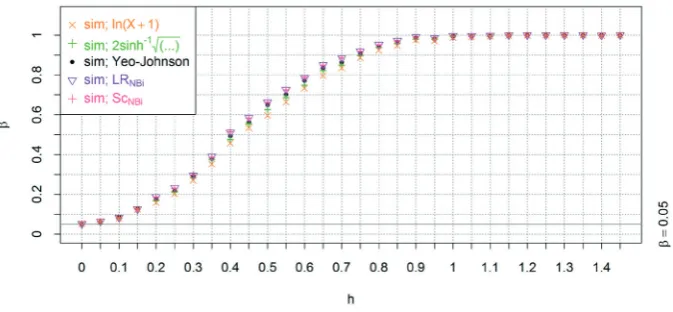
We will continue by presenting the graphical comparison of simulated power functions. Out of the multitude of computational results for various choices of parameters, we will present the cases for the following pairs of parameters
θ1 = 5, κ = 3; θ1 = 5, κ = 10; θ1 = 100, κ = 10; and θ1 = 50, κ= 5. The reason for the choice of
the first pair is to observe, how the methods of the different approaches tackle with the worst case scenario – a relatively small expectation parameter and a small shape parameter. The second pair represents the case of a relatively small value of the expectation parameter but relatively big value of the shape parameter. The third pair represents the choice of big values of both parameters and
finally, the last pair represents the choice of moderately big expectation and shape parameters. Additionally, for the case and the comparison is enriched by the theoretical power functions for samples transformed via (4) and (7) (see Fig. 9, red and blue lines respectively). For the other two cases that are covered in the graphical comparison, the theoretical power functions are not presented because the approximations of numerical characteristics used in the computations do not behave well (for more detail see Tejkal, 2017).
From the Figures 6, 7, and 9 we can see that the worst performance regardless of the setting of the parameters has the transformation (4). In case of small shape parameter κ (see Fig. 6), the difference between (4) and (7) is not very significant. However, in case of big value of the shape parameter κ (see Fig. 7) (7) performs better than (4). This ceases to be true for big values of the expectation parameter θ (see Fig. 8). The best performance out of the approach via transformations has transformation (6).
6: Negative binomial case – Power functions comparison for κ = 3, θ1 = 5, θ2 = θ1 + h, θ3 = θ1 – h
8: Negative binomial case – power functions comparison for κ = 10, θ1 = 100, θ2 = θ1 + h, θ3 = θ1 – h
9: Negative binomial case – power functions comparison for κ = 5, θ1 = 50, θ2 = θ1 + h, θ3 = θ1 – h
10: Negative binomial case – power functions as functions of a sample size at hj = 7.98 (approximately a half of the computation interval) for
Notice also, that for a good performance of a transformation it seems to be more important, that the skewness of the transformed sample is close to 0, than that the variances among the samples are equal. Observe that (6). that performs the best out of the considered transformations, does not stabilise variance in the particular studied case (see Fig. 4), however, the skewness of samples transformed via (6) is close to 0 (see Fig. 5).
Using test statistic coming from the theory of maximum likelihood seems to be the best approach since the power function of the test when either (13) or (14) is used attains higher values than any power function of the approach via transformations. The simulated power function of the test statistic (14) tends to attain slightly higher values than the one of (13). We may further observe, that for increasing values of θ and κ the differences between the power functions become smaller (cf. Fig. 6 with 9, and 6 with 7).
Lastly, we will present the graphical comparison of the power functions for different sample sizes for all the studied approaches. Recall that the value of hj is the difference between the fixed θ1 and
the computed θ2 and θ3 respectively.
From Fig. 10 we can observe, that for the best performing method (likelihood ratio test statistic (13)), to distinguish the difference hj = 7.98 with probability β = 0.8, samples of a size n = 23 are needed. For the worst performing pair of methods (logarithmic transformation (4) and argument of hyperbolic sine transformation (7)), to distinguish the difference hj = 7.98 with probability β =0,8, samples of a size n = 28 are needed.
DISCUSSION
The early trend in tackling the non‑normal heteroscedastic data involving counts in linear regression and the respective tests was to apply various transformations in order to achieve normality and homoscedasticity. To improve the desired effect
of the transformations of the random variables with Poisson and negative binomial distribution, Anscombe (1948) introduced generalisations of the variance stabilising transformations. For data involving counts it is often convenient to use the logarithmic scale, therefore the logarithmic transformation comes, perhaps, as a natural choice. The problem of zero observations is usually solved by adding a constant (usually one) into the argument of the logarithm. Some authors even suggest different constants. Anscombe (1948) derives the logarithmic transformation for negative binomially distributed random variable as an approximation of the more complicated argument of hyperbolic sine transformation and finds an optimal value of the constant added within the argument to be a function of the shape parameter κ of the distribution. Yamamura (1999) suggests using transformation Y = ln(X + 0.5) instead of Y = ln(X + 1). Numerical analysis carried out when collecting data for this paper, however, did not suggest, that there is a significant improvement in the power of the test when Anscombe’s or Yamamura’s choice of the optimal constant was used instead of adding one within the argument of the logarithm. On the other hand, the family of transformations developed by Yeo and Johnson (2000) performed in our comparison significantly better than both the logarithmic transformation with one added within the argument or the transformations proposed by Anscombe.
More recent development (see O’Hara and Kotze, 2010) has shown that for modelling data involving discrete counts, models based on Poisson or negative binomial distribution attain better results than the approach via transformations. The results of this paper in general support this statement. The GLM based tests outperformed the approach via transformations in all studied cases. However, for some cases, the difference between the GLMs and the approach via Yeo‑Johnson transformation, the best performing one out of the studied transformations, was rather small.
CONCLUSION
The presented analysis provides a comparison of different methods of testing the hypothesis of equality of expectations for data involving counts. Poisson and negative binomial distributions were used to model the data. Two main approaches were used, the approach via normalising and variance stabilising transformations, followed by applying the classical ANOVA towards the transformed data, and the approach via GLM test statistics.
In the Poisson case, the GLM test statistics performed better than the transformational approach. By far the highest values were attained by the simulated power function of the score test statistic (12) followed by the power function of the likelihood ratio test statistic (11). The likelihood ratio test statistic, in turn, performed slightly better than any of the transformations. It should be noted, however, that the score test tends to have greater simulated test size than the chosen level of significance α = 0.05, since the respective power function did not attain the value 0.05 for h = 0. The square root (5) and the Yeo‑Jonnson transformation (6) both performed similarly and both better than the logarithmic (4) transformation, which performed the worst. With increasing values of the expectation parameter
θ of the Poisson distribution, the differences between the power functions of the different approaches became negligible.
the GLM test statistics were used. The simulated power function of the score statistic (14) attained higher values than the one of the likelihood ratio statistic (13). All of the transformations performed worse than the GLM test statistics. The Yeo‑Johnson transformation (6) outperformed the argument of hyperbolic sine transformation (7) and the logarithmic transformation (4). The argument of hyperbolic sine achieved better results than the logarithm for small values of θ and big values of κ. The difference between these two transformations for small values of θ and κ and for big values of θ
independently of κ were not significant. For increasing values of the parameters θ and κ the differences between the power functions of the different approaches became negligible.
Finally, by comparing the power functions for different sample sizes we saw, that by choosing the right approach, we can obtain a given power of the test with significantly smaller sample, than in the case of picking a less suitable approach. Namely, the difference between the worst and best performing method in the comparison provided in this paper was 10 samples in the Poisson case and 5 samples in the negative binomial case.
REFERENCES
ANDĚL, J. 2011. Basics of mathematical statistics [in Czech: Základy matematické statistiky]. Praha: Matfyzpress. ANSCOMBE, F. J. 1948. The transformation of Poisson, binomial and negative binomial data. Biometrika,
35(3–4): 246–254.
HRDLIČKOVÁ, Z. 2006. Comparison of the power of the tests in one‑way ANOVA type model with Poisson distributed variables.Environmetrics, 17(3): 227–237.
HRDLIČKOVÁ, Z. 2008. Approximation of powers of some tests in one‑way MANOVA type multivariate generalized linear model.Computational Statistics & Data Analysis, 52(8): 4059–4075.
HRDLIČKOVÁ, Z. 2002. Log‑linear models with Poisson random variables [in Czech: Log‑lineární modely s Poissonovskými proměnnými]. Diploma Thesis. Masaryk University in Brno, Faculty of Science. Supervisor: doc. RNDr. Jaroslav Michálek, CSc.
HÜBNEROVÁ, Z. and DOUDOVÁ, L. 2011. Influence of estimate of shape parameter on tests in models with negative binomial distribution. In: Biometric Methods and Models in Current Science and Research. Brno: UKZUZ, pp. 119–126.
O’HARA, R. B. and KOTZE, D. J. 2010. Do not log‑transform count data.Methods in Ecology and Evolution, 1(2): 118–122.
MOSS, D. and MCPHEE, D. P. 2006. The impacts of recreational four‑wheel driving on the abundance of the ghost crab (Ocypode Cordimanus) on sub‑tropical sandy beaches in SE Queensland.Coastal Management, 34: 133–140.
SCHEFFÉ, H. 1999. The analysis of variance. Wiley classics library ed. New York: Wiley‑Interscience Publication. TEJKAL, M. 2017. Selected random variables transformations used in classical linear regression. Diploma thesis.
Brno University of Technology, Faculty of Mechanical Engineering. Supervisor: Doc. Mgr. Zuzana Hübnerová, Ph. D.
YAMAMURA, K. 1999. Transformation using (x + 0.5) to stabilize the variance of populations.Researches on Population Ecology, 41(3): 229–234.
YEO, I., and JOHNSON R. A. 2000. A new family of power transformations to improve normality or symmetry. Biometrika, 87(4): 954–959.
Contact information Martin Tejkal: [email protected]