Arctic sea ice and ocean topography from satellite altimetry

Arctic Sea Ice and Ocean Topography

from Satellite Altimetry

Neil Robert Peacock

A thesis submitted to the University of London for the degree of

Doctor of Philosophy

Mullard Space Science Laboratory

Department of Space and Climate Physics

University College London

ProQuest Number: U643155

All rights reserved

INFORMATION TO ALL USERS

The quality of this reproduction is dependent upon the quality of the copy submitted.

In the unlikely event that the author did not send a complete manuscript and there are missing pages, these will be noted. Also, if material had to be removed,

a note will indicate the deletion.

uest.

ProQuest U643155

Published by ProQuest LLC(2016). Copyright of the Dissertation is held by the Author.

All rights reserved.

This work is protected against unauthorized copying under Title 17, United States Code. Microform Edition © ProQuest LLC.

ProQuest LLC

789 East Eisenhower Parkway P.O. Box 1346

$

Frontispiece Arctic ice thickness distribution for December 1996

Abstract

T his th esis explores novel applications o f data from the ERS-1 and 2 satellite

altim eters in the Arctic. The use of such data in this region has been restricted in the

past by the presence o f sea ice, which vastly affects the radar écho received from the

surface. The altim eter instrum ents are optimised for operation in ice-free seas, w hich

gen erate diffuse, low pow er echoes. W hen sea ice is p resen t, h igher po w ered

specular echoes are observed. Evidence is presented to support the hypothesis that

these echoes originate from regions of calm w ater between ice floes, thus allow ing the

direct m easurem ent o f sea surface height in areas of very high ice concentration.

R esults from a full sim ulation of the ERS altim eter tracking system have enabled the

developm ent o f processing algorithm s which dram atically reduce short w avelength

instrum ent noise. This has enabled direct m easurem ents of sea surface height to be

m ade for the first tim e in ice-covered seas. M aps o f sea surface height variability and

eddy kinetic energy are presented, and compared with the corresponding output from

two A rctic Ocean models. An empirical tide model based purely on the altim eter data

has also been developed and is compared with existing models.

O pen ocean-like echoes have been observed in areas o f 100% ice cover, and are

show n to o rig in ate from the surfaces o f ice floes. T h e a sso c ia te d h eig h t

m easurem ents are seen to deviate from those o f the surrounding w ater by an am ount

w hich is attributed to ice elevation. From these m easurem ents, estim ates o f ice

thickness have been m ade, allowing the first direct large-scale observations o f this

param eter from space. A preliminary validation of these m easurem ents is perform ed

Acknowledgements

I w ould first like to thank Dr. Seym our Laxon for his ex cellent supervision and

guidance throughout the course of my studies, and for his thorough review o f this

thesis. I have benefited enorm ously from his enthusiasm for the subject, and his total

com m itm ent to seeing a successful outcome to this work. M y thanks also extend to

the other m em bers o f the Climate Physics Group, past and present, for their ideas and

com m ents w hich have helped along the way, in particular Justin M ansley for all his

hard work. I should also thank the many other people from outside M SSL w ho have

either provided m e w ith data or direction for my work. T hanks also to N E R C for

their financial support o f my project under grant num ber G T4/95/209/EO .

I am also grateful to the past and present students at M SSL w ho have prov id ed a

w elcom e break from work. In particular, cheers to G az and Laz for their excellent

com pany and beer drinking skills. My gratitude also extends to my friends M artin

and Linda who have so willingly opened up their hom e to me to allow m e to com plete

m y PhD w ithout having to worry about where to live.

An enorm ous thank you m ust also go to my M um and D ad w ho have given m e their

w holehearted support during the course of my education. T heir encouragem ent and

w isdom in all sorts o f areas has been invaluable to me. Thanks also to T heresa for her

support during the last few months of my studies, and for putting up w ith m e during

this time. I can't w ait for you to becom e my wife in July - I'll always love you!

Finally, I thank the L ord for His faithfulness tow ards m e and the m any blessings I

have received from H im throughout my life. I acknow ledge G od as the C reator o f the

U niverse, o f w hich I have had the privilege of studying a very sm all part.

"The earth is the Lord's, and everything in it, the w orld, and all who live in it; for he

Acknowledgements

I w ould first like to thank Dr. Seym our L axon for his ex cellent sup ervision and

guidance throughout the course o f my studies, and for his thorough review o f this

thesis. I have benefited enorm ously from his enthusiasm for the subject, and his total

com m itm ent to seeing a successful outcom e to this work. M y thanks also extend to

the other m em bers o f the Clim ate Physics Group, past and present, for their ideas and

com m ents w hich have helped along the way, in particular Justin M ansley for all his

hard work. I should also thank the m any other people from outside M SSL w ho have

either provided me w ith data or direction for my work. Thanks also to N E R C for

their financial support o f my project under grant num ber G T4/95/209/EO .

I am also grateful to the past and present students at M SSL w ho have p ro v id ed a

w elcom e b reak from work. In particular, cheers to Gaz and Laz for their excellent

com pany and beer drinking skills. My gratitude also extends to my friends M artin

and L inda w ho have so willingly opened up their home to me to allow me to com plete

my PhD w ithout having to worry about where to live.

An enorm ous thank you m ust also go to my M um and D ad who have given m e their

w holehearted support during the course o f my education. T heir encouragem ent and

w isdom in all sorts o f areas has been invaluable to me. Thanks also to T heresa for her

support during the last few m onths o f my studies, and for putting up w ith m e during

this time. I can't w ait for you to becom e my wife in July - I'll always love you!

F inally, I thank the L ord for H is faithfulness tow ards m e and the m any blessings I

have received from H im throughout my life. I acknow ledge G od as the C reator o f the

U niverse, o f w hich I have had the privilege o f studying a very sm all part.

"The earth is the Lord's, and everything in it, the world, and all who live in it; for he

List of contents

Title page

1

Frontispiece

2

Abstract

3

Acknowledgements

List of contents

6

List of figures

List of tables

Chapter 1

The Arctic climate system

1.0 Introduction 15

1.1 The global clim ate system 16

1.1.1 C om ponents o f the global climate system 16

1.1.2 Global climate change 17

1.1.3 Global clim ate models 19

1.2 Influence o f the Arctic on the global clim ate system 19

1.2.1 The global thermohaline circulation 19

1.2.2 O cean-ice-atm osphere interactions 21

1.2.3 Radiation balance of the Earth's surface 22

1.3 Circulation and structure of the Arctic Ocean 23

1.4 Characteristics of Arctic sea ice 26

1.4.1 Physical properties of sea ice 26

1.4.2 Seasonal variability of ice extent 28

1.4.3 Ice thickness distribution 28

1.5 M odelling Arctic processes 29

1.5.1 A review o f coupled ice-ocean m odels 29

1.5.2 Global climate models and their representation o f the A rctic 32

1.6 M onitoring the Arctic climate svstem 32

1.6.1 In situ observations of ocean circulation 33

1.6.2 D ata requirem ents for sea ice m onitoring 34

1.6.3 Rem ote sensing of sea ice 35

1.6.3.1 Ice extent and concentration 35

1.6.3.2 Ice motion 36

1.6.3.3 Ice thickness 37

1.6.3.4 Ice albedo and surface m elting 37

1.7 Summary 39

Chapter 2

Geophysical applications of satellite radar altimetry

2.0 Introduction 41

2.1 Fundam ental principles o f altimetry 42

2.1.1 The concept o f altim etry 42

2.1.2 Corrections in altim eter data processing 44

2.1.2.1 Satellite orbital position 45

2.1.2.2 A tm ospheric corrections 45

2.1.2.3 Tidal corrections 46

2.1.2.4 Inyerted barom eter effect 48

2.1.3 Past, present and future altim eter missions 49

2.2 Oceanographic applications o f altimetry 52

2.2.1 Studies o f m esoscale ocean processes 52

2.2.2 O bservations o f large-scale ocean circulation 52

2.2.3 V alidation o f ocean general circulation m odels 53

2.2.4 D eyelopm ent o f ocean tide models 54

2.3 Exploitation o f satellite altimetry in the Arctic Ocean 55

2.3.1 M easurem ent o f grayity anomalies 55

2.3.2 Ocean circulation studies and model yalidation 57

2.3.3 Ice extent and freeboard determ ination 57

2.4 Sum m ary and aims o f this study 58

Chapter 3

The ERS-1 and 2 radar altimeter systems

3.0 Introduction 60

3.1 O yeryiew of the ERS m issions 60

3.2 A ltim etry principles 62

3.2.1 Pulse-lim ited altim etry 62

3.2.2 Pulse transm ission and reception 63

3.2.3 The conyolutional w ayeform m odel 65

3.2.4 W ayeform ayeraging and tracking 68

3.3 The ERS tracking system 68

3.3.1 System oyeryiew 68

3.3.2 Sam pling o f return signals 70

3.3.3 Param eter error estimation 71

3.3.4 Tracking loop filters 74

3.4 ERS altim eter data products 77

3.4.1 ERS W aveform Product 77

3.4.2 ERS O cean Product 78

3.5 Sum m ary 79

Chapter 4

Retrieval of accurate altimetric height measurements

in ice-covered seas

4.0 Introduction 80

4.1 Origins o f the waveforms found in sea ice altim eter data 80

4.2 Sea surface height data processing 85

4.2.1 W aveform filtering scheme 85

4.2.2 W aveform categorisation 85

4.2.3 Retracking algorithms 87

4.2.4 Categorisation of diffuse w aveforms 88

4.2.5 H eight estimate quality controls 89

4.2.6 A long-track interpolation and filtering 89

4.2.7 Resam pling o f processed data 89

4.2.8 Orbit error reduction 90

4.3 Sim ulation o f the ERS tracking system 90

4.3.1 D escription o f the simulation software 90

4.3.1.1 M ain tracking module 91

4.3.1.2 SM LE algorithm 92

4.3.1.3 W aveform generator 92

4.3.2 Sim ulation results over open ocean 94

4.3.3 Sim ulation results over sea ice 95

4.3.4 Theoretical performance of the H TL over sea ice 97

4.4 A pplications o f the simulation results to data processing 101

4.4.1 Pulse blurring correction 101

4.4.2 Retracking bias correction 102

4.5 A ssessm ent o f improvements to altimeter data 106

4.5.1 Crossover analysis 106

4.5.2 A nalysis o f collinear tracks 107

4.5.3 Sea surface height measurement error budget 108

4.6 G eneration o f an Arctic mean sea surface 110

Chapter 5

Development and assessment of an Arctic tide model

5.0 Introduction 114

5.1 O verview of tidal constituents 114

5.2 O bservations o f tides using altimetrv 115

5.2.1 Tidal aliasing 115

5.2.2 The ERS aliasing problem 116

5.3 G enerating the ERS tide model 117

5.3.1 Preparation of altimeter data 117

5.3.2 The response method 118

5.3.3 D eriving amplitudes and phases o f tidal constituents 120

5.4 A ssessm ent o f the ERS tide model 122

5.4.1 Com parisons with existing tide models 122

5.4.2 Com parisons with tide gauge m easurem ents 125

5.5 A pplication o f tide models to altimeter data processing 130

5.6 Conclusions 131

Chapter 6

Observations of sea surface height in the Arctic Ocean

and comparisons with models

6.0 Introduction 133

6.1 D escription o f the ocean models 133

6.1.1 O CCAM 134

6.1.2 NFS 135

6.1.3 Com parisons between the models 135

6.2 Sea surface height variability 136

6.2.1 Variability from altimetry 136

6.2.2 M odel variability and comparisons w ith altim etry 138

6.2.3 Sea surface height wavenumber and frequency spectra 140

6.3 Eddy kinetic energv 143

6.3.1 Eddy kinetic energy from altimetry 143

6.3.2 M odel eddy kinetic energy and com parisons w ith altim etry 145

6.4 The seasonal cvcle 146

6.4.1 M onthly sea surface height anom alies 147

6.4.2 Seasonal sea surface height anom alies 149

6.4.3 A nnual harmonic in sea surface height 149

Chapter 7

Estimating sea ice thickness in the Arctic

7.0 Introduction 154

7.1 M ethod o f ice thickness determination from altim etrv 154

7.1.1 The origins of diffuse and specular w aveform s 154

7.1.2 H eight anomalies from diffuse w aveform s 155

7.1.3 Estim ating ice thickness from elevation m easurem ents 157

7.2 A ccuracv and limitations of the method 158

7.3 M onthly ice thickness maps 162

7.4 V alidation w ith upward-looking sonar data 167

7.5 A pplications o f the ice thickness estimates 172

7.5.1 Latitudinal dependence of ice ablation 172

7.5.2 Com parisons with the predictions o f a sea ice m odel 174

7.5.3 Seasonal and inter-annual variations in ice thickness 174

7.6 Conclusions 176

Chapter 8

Conclusions

8.0 Introduction 178

8.1 A ssessm ent o f achievements 178

8.1.1 Primary objectives 178

8.1.2 Sum m ary o f key results 180

8.2 D irections for future work 182

8.2.1 M odelling radar backscatter in sea ice-covered regions 182

8.2.2 A ssim ilation o f altimeter data into existing ocean tide m odels 183

8.2.3 A ltim eter and ocean model com parisons 183

8.2.4 Im proved estimates and validation o f ice thickness 183

8.2.5 Im provem ents to current polar gravity fields 184

8.2.6 Extending the work to studies of the A ntarctic region 185

8.3 Future spaceborne altim eter missions in the polar regions 185

List of acronyms

187

References

189

List of figures

Chapter 1

1.1 The clim ate system 16

1.2 G lobal tem perature variations 18

1.3 Carbon dioxide concentrations over the past 1000 years 18

1.4 The great ocean thermohaline conveyor belt 20

1.5 Sea ice albedo feedback mechanism 23

1.6 Surface circulation features of the Arctic Ocean 24

1.7 Circulation and w ater mass structure in the A rctic 25

1.8 A rctic pack ice from an altitude of 10,000 m etres 27

1.9 Physical properties o f various sea ice types 27

1.10 Sea ice concentration in the Arctic from SSM /I 28

1.11 Contours o f mean ice draft 30

Chapter 2

2.1 The altim eter measurement system 43

2.2 M odel vector differences for the M2 constituent 48

2.3 Tim escale and coverage of altimeter missions 51

2.4 G ravity field o f the Arctic Ocean from ERS-1 56

Chapter 3

3.1 ERS-1 and 2, and EN VIS A T -1 mission configurations 61

3.2 G eom etry for pulse-lim ited altimetry 62

3.3 Full deram p processing method 64

3.4 Typical ERS-1 altim eter waveforms 65

3.5 Construction o f a return echo over open ocean 66

3.6 The ERS tracking system 69

3.7 The ERS range window 70

3.8 ERS SM LE gate configuration 72

3.9 A second order low-pass aj3-filter 76

Chapter 4

4.2 C oincident altim eter track and ATSR-2 thermal im age 84

4.3 Sea surface height data processing scheme 86

4.4 Threshold re tracking scheme for specular w aveform s 88

4.5 A long-track resam pling of data points 90

4.6 Construction o f synthesised diffuse and quasi-specular w aveform s 94

4.7 D istributions o f the height error signal 95

4.8 H TL error signal versus retracked height error 97

4.9 A long-track retracked heights and HTL error signals 98

4.10 H eight error signal versus 99

4.11 Positions of average waveforms relative to centre o f range w indow 100

4.12 Sequences o f waveforms synthesised using the convolutional m odel 103

4.13 Relationship between peakiness and retracking bias 104

4.14 M ethod used to estimate specular-diffuse bias 105

4.15 Peakiness versus retracking bias for specular w aveform s 105

4.16 C rossover differences for ERS-2 107

4.17 C ollinear track differences from ERS-1 and 2 108

4.18 D ifference betw een ERS-2 mean sea surface and O SU M SS95 111

4.19 D ifference between ERS-2 mean sea surface and EG M 96 112

Chapter 5

5.1 A m plitudes and phases of the M] and K, constituents 122

5.2 V ector differences between ERS and F E S 95 .2 .1 tide m odels 124

5.3 Locations o f coastal and pelagic tide gauge stations 126

5.4 Com parisons between ERS tide model and gauge m easurem ents 128

Chapter 6

6.1 Sea surface height variability from ERS-2 138

6.2 Sea surface height variability from OCCAM and N PS m odels 139

6.3 Zonal averages o f variance between 70°N and 80°N . 141

6.4 W avenum ber and frequency power spectra 142

6.5 Eddy kinetic energy in the Arctic from ERS-2 144

6.6 Eddy kinetic energy from the OCCAM and NPS m odels 146

6.7 M onthly averaged sea surface height residuals 148

6.8 Seasonal sea surface height anomalies 150

6.9 A nnual sea surface height signal 151

Chapter 7

7.1 Peakiness and residual elevations over an ice floe 156

7.2 N um ber and distribution of diffuse echoes from ERS-2 160

7.3 Ice thicknesses for Decem ber 1996 from ERS-2 162

7.4 Contours o f m ean ice draft from submarine ULS m easurem ents 164

7.5 Ice thicknesses for M arch from ERS-2 and clim atology 165

7.6 Ice thicknesses for April 1996 from ERS-1 and 2 165

7.7 M onthly maps of ice thickness from ERS-2 166

7.8 Locations and periods of operation of A ITP ULS stations 167

7.9 Tim e series o f ice thicknesses from ULS and ERS-1 and 2 168

7.10 Frequency distribution of ice thickness from ERS-2 and ULS 170

7.11 Zonally averaged ice thickness from ERS-2 173

7.12 M onthly maps o f ice thickness from the NPS m odel 175

List of tables

Chapter 1

1.1 Freshw ater budget for the Arctic Ocean 21

1.2 D ata requirem ents for sea ice monitoring 34

1.3 Instrum ents used in the remote sensing of sea ice 35

Chapter 2

2.1 V ertical ranges of some oceanographic phenom ena 44

2.2 Past, present and future spaceborne altim eter m issions 50

Chapter 3

3.1 ERS SM LE gate configuration 72

3.2 E R S -1 and 2 ccjS-filter parameters 75

Chapter 4

4.1 Sea ice altim etry height error budget 109

Chapter 5

5.1 M ain low frequency tidal constituents 115

5.2 M ain sem idiurnal and diurnal tidal constituents 116

5.3 O rthotide coefficients 121

5.4 rms differences betw een various tide models 125

5.5 Com parisons between ERS tide model and gauge m easurem ents 129

5.6 Com parisons betw een various tide models and gauge m easurem ents 130

5.7 rm s crossover differences for ERS-2 with various tide m odels 131

Chapter 6

6.1 Sum m ary o f the OCCAM and NFS ocean m odels 136

6.2 V ariabilities from ERS-2 and ocean models 140

6.3 Eddy kinetic energy from ERS-2 and ocean m odels 147

6.4 A nnual signal from ERS-2 and ocean models 152

Chapter 1 The Arctic climate system

1.0 Introduction

The m ain aim o f the work presented in this thesis is to exploit the use o f satellite radar

altim etry in the A rctic O cean as a means o f m easuring param eters o f fun dam ental

im portance to studies o f the clim ate system. The A rctic region is a key com ponent o f

the global clim ate system , prim arily through its effects on the E arth's su rface h eat

balance and global therm ohaline circulation [Aagaard an d C arm ack, 1994]. T here

are m any potential clim atological applications of this w ork, som e o f w hich are listed

here:

• A R C TIC O CEA NO G RAPH Y - studies o f m esoscale and large-scale sea

surface height variability on intra-seasonal, seasonal and in ter-an n u al

tim e-scales.

• O C EA N M O D EL V A LID A TIO N - com pariso n o f the v aria b ility and

energy content on a range of temporal and spatial scales.

• C LIM A TO LO G Y - m easurem ents of A rctic sea ice thicknesses for the

monitoring o f global climate change.

• SEA ICE M O D E L V A LID A TIO N - com parison o f the tem p o ral and

spatial variations o f sea ice thickness.

This w ork has also enabled the development of:

• An Arctic Ocean tide model, the predictions o f w hich have been com pared

with those o f other models and in situ tide gauge m easurem ents.

• An accurate Arctic m ean sea surface, w hich is a vital starting point for the

above applications of altimeter data.

1.1 The global clim ate svstem

1.1.1 C om ponents o f the global climate system

The clim ate system consists of five com ponents, all o f w hich interact th ro u g h

complex and often non-linear processes [Cubasch and Cess, 1990]:

(i) atmosphere

(ii) ocean

(iii) cryosphere

(iv) biosphere

(v) geosphere

A schematic representation of this system with its internal processes and interactions can be seen in figure 1.1, along with sources of natural and anthropogenic external

forcing.

C h a n g e s in S olar Inputs

S \

C h a n g e s in the H ydrological Cycle C h a n g e s in I he A tm osphere

Composition, Circulation

A tm osphere _Clouds

Aerosols

HjO. Nr. O r. CO;, Oj. etc A ir-Biom ass Coupling

Precipitation- Terrestrial Evaporation Radiation H eat Wind

E xchange S tre ss

Human Influenc_

B iom ass L and-B iom ass

Coupling Rivers

L a k e s O cean

C oupling i

C h a n g e s in th e O cean: Circulation. Biogeochem istry

C h a n g e s in/on th e Land Surface: O rography. L and U se. Vegetation. E co sy stem s

F ig u re 1.1 A schem atic view of the climate system . Internal processes and

interactions are represented by the thin arrows, and the bold arrows show exam ples of aspects that may change (from Trenherth et al. [1996]).

Each com ponent o f the climate system reacts to external forcing w ith varying degrees

o f rapidity [Cubasch and Cess, 1990]. For exam ple, the atm osphere responds to its

forcing on a tim escale o f hours or days, whereas the ocean responds on tim escales

ranging from days for the surface layer to m illenn ia in the deep ocean. In the

cryosphere, a w hole spectrum o f timescales can be found, ranging from days for sea

ice, to m illennia for ice sheets. Land processes in the geosphere react on tim escales o f

days to m onths, w hile the biosphere can react on tim escales o f hours (p lank to n

grow th) to centuries (tree growth). The sea ice com ponent o f the clim ate system is

therefore influenced relatively rapidly by external factors.

1.1.2 Global climate change

The clim ate is a naturally varying system, with tim escales ranging from hundreds o f

m illions o f years to a few years [Folland et a l, 1990]. This is the result o f internal fluctuations in the chaotic system , and changes in external forcing, such as solar

variability or volcanic eruptions [IPCC, 1994]. F igu re 1.2 show s schem atically

variations o f global tem perature on three different tim escales. Since the late 19th

century to the present, global mean surface air tem peratures have risen by betw een 0.3

and 0.6°C with a corresponding increase in sea level o f betw een 10 and 25 cm [IPCC,

1995].

The influence o f m ankind on the global climate is difficult to ascertain, as it w ill be

superim posed on the background signal of natural clim ate variability. In spite o f this,

the available evidence suggests a discernible anthrop og en ic influence on glob al

clim ate [7PCC, 1995]. A m ajor factor in hum an-ind uced clim ate chan ge is the

increase in concentration o f greenhouse gases, such as carbon dioxide, m ethane and

chlorofluorocarbons. The result of these concentration increases is an en h anced

greenhouse effect, above that due to the presence o f natural concentrations o f such

ü

i

I

Y ears before p resen t 200,000 O (b) Little & age 0 2

1

I

Years before p resen t

2.000 0 10,000

Ü

& L ittle Ic e a g e

I

i

1000 AD 1500 AD Years before p rese n t

1900 AD

Figure 1.2 Schematic global temperature variations on three different timescales: (a)

the last million years, (b) the last ten thousand years, and (c) the last thousand years.

The dashed line represents the temperature at the beginning of the twentieth century

(from Folland et a l [1990]).

380

360

340

320

c 300

280

260 800

# D57

f S l p l e

• South Pole Mauna Loa Fossil CO2 emissions .— One hundred year

running moan ^ ? 3 G 0

2000

Figure 1.3 Carbon dioxide concentrations over the past 1000 years from ice-core

records (D47, D57, Siple and South Pole), and since 1958 from the M auna Loa,

Hawaii measurement site (from IPCC [1994]).

1.1.3 Global climate models

In order to assess the response o f the clim ate system to different external forcing,

coupled general circulation models (CGCMs) have been developed w hich are able to

m odel large-scale effects with a reasonable level o f skill [Gates et a i , 1996]. These m odels include representations of the atmosphere, ocean, cryosphere and land surface,

and their interactions.

T he usefulness o f these models lies in their ability to estim ate the effects o f changes

in greenhouse gas forcing on global surface air tem perature. F or exam ple, the IPC C

selec ted six greenhouse gas scenarios in order to m odel th e ir effect on g lo bal

tem perature [7PCC, 1992]. The results show ed an increase in global surface air

tem perature o f betw een T C and 3.5°C by 2100 in the b est and w orst case scenarios

resp ectiv ely [IPC C , 1995]. O ther models p redict d ifferent tem peratu re changes.

W ashington and M eehl [1996] used a global coupled ocean -atm osphere-ice m odel w ith C O2 increasing at 1% per year com pounded for 75 years to pred ict a globally

averaged surface air tem perature of 3.8°C at the time o f CO2 doubling.

T he developm ent o f CG CM s has increased rapidly since 1990 as ch eaper and m ore

pow erful com puters have becom e available, and the current generation o f m odels are

able to sim ulate the observed climate with a reasonable level o f skill. C onsiderable

u n certainties do still rem ain, and large, poorly understood discrepancies have been

o b serv ed in the predictions o f different m odels. In spite o f this, the an ticip ated

advances in our m odelling capability over the next few years w ill provide us w ith the

m ost pow erful tool available for the assessment o f future clim ate.

1.2 Influence of the Arctic on the global climate svstem

1.2.1 The global thermohaline circulation

T he A rctic O cean is know n to have a sig nificant in flu en ce on the larg e -sc ale

therm oh aline circulation o f the w orld ocean [JSC Study G roup on A C S Y S , 1992;

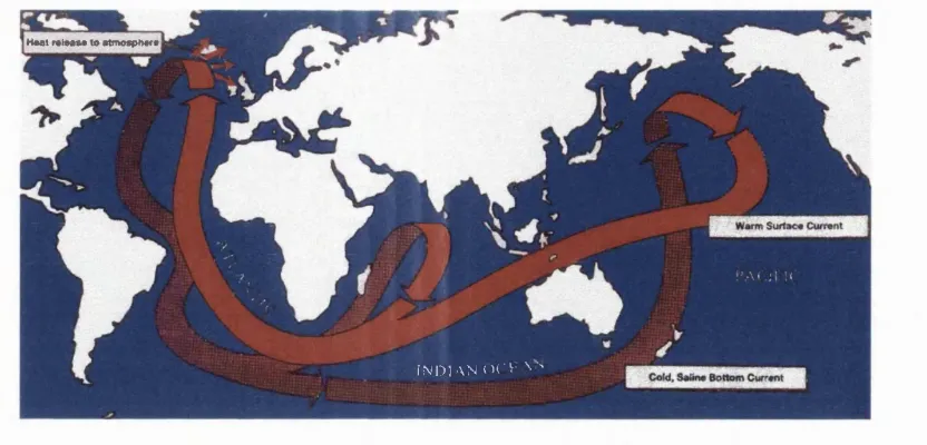
A a g a a r d a n d C a rm a ck, 1994], w hich is an im p o rtan t m ode o f g lo b a l heat redistribution. Figure 1.4 shows a schematic diagram o f w hat has becom e know n as

the great ocean therm ohaline conveyor belt, indicating the path o f th is circu lation

Meet r#*e#w to «tmotphort

I N D I A N D C V - A '

Figure 1.4 Schematic diagram of the great ocean thermohaline conveyor belt (from

JSC Study Group on ACSYS [1992]).

In this figure, the north Atlantic is shown as a region of ocean overturning, as a result

of the densification of water due to cooling at high latitudes [Dickson et a i, 1990]. A vast amount o f heat is released to the atm osphere by this deep w ater form ation,

corresponding to about 30% o f the solar heat reaching the surface o f the Atlantic

Ocean north o f 35°N [Broecker et al., 1985]. It is thought the changes in this

overturning, and hence heat release to the atm osphere, were responsible for past

climate change. For example, Broecker et al. [1985] discuss the possibility that the anom alous cooling in Europe during the Y ounger Dry as event was caused by a

weakening of the thermohaline circulation.

A agaard and Carmack [1989] suggest that the present-day G reenland and Iceland Seas are delicately poised with respect to their ability to sustain convection. These

convective gyres are thought to be conditioned by freshwater export from the Arctic

Ocean via the East G reenland Current, and that small variations in this export can

alter or stop the convective overturning. A significant increase in export would most

likely dim inish convection, whereas a decrease in export would result in m ore

vigorous convection [Aagaard and Carmack, 1994].

In the late 1960s, a significant freshening of the upper ocean north o f Iceland was

observed, resulting in a freshening and cooling o f the North A tlantic Deep W ater.

A aga ard and Carm ack [1989] hypothesised that this so-called "Great Salinity Anomaly" was the result o f an increase in the freshwater discharge from the Arctic

Ocean. Hakkinen [1993] confirm ed that the A rctic was indeed the source o f this

anomaly through a simulation of the ice-ocean system over the period 1955 to 1975.

F resh w ater export from the A rctic in the form o f both ice and w ater in 1968 w as

found to be anom alously high. Aagaard and Carm ack [1994] describe this event as

th e m o d e rn d ay e q u iv a le n t o f a h a lo c lin e c a ta s tr o p h e , p ro p o s e d by

paleoclim atologists, in w hich the convective gyres are capped by freshwater.

Table 1.1 shows the freshw ater budget for the Arctic Ocean, and highlights the extent

o f the freshw ater export through Pram Strait, predom inantly in the form o f sea ice, to

the convective gyres to the south.

Source or sink T ransport (k m ^ y r^

Ice export through Fram Strait -2790

W ater export through Fram Strait -820

R unoff 3300

Precipitation less evaporation 900

W ater im port through Bering Strait 1670

W ater export through Canadian Archipelago -920

Im port w ith N orw egian Coastal Current 250

Saline w ater im port through Barents Sea -540

Saline w ater im port with W est Spitsbergen Current -160

N et 890

T able 1.1 Freshw ater budget for the Arctic Ocean. V alues are positive for sources

and negative for sinks (from Aagaard and Carmack [1989]).

A a g a a rd and C arm ack [1989] suggest that the apparent im balance in the bu dget, m anifest as a net surplus o f freshwater, is probably indistinguishable from zero, after

uncertainties in the contributing terms have been taken into account.

1.2.2 Ocean-ice-atmosphere interactions

T he o cean -ice-atm o sp h ere system in the A rctic is in tim a tely co u p led , an d an

understanding o f the surface heat balance, the sea ice m ass balance, surface radiative

properties, and interactions betw een the three com ponents is essential for accurately

sim ulating present and future Arctic climate [Moritz and Perovich, 1996].

T he su rface energy balance is determ ined by the absorbed in solatio n, net long

w avelen gth radiation , atm ospheric sensible and laten t h eat fluxes, and th e heat

G roup on AC SYS, 1992]. The presence or absence o f sea ice is an im portant factor in determ ining this balance for two m ain reasons: (i) sea ice is an effective b arrier to

sensible and latent heat fluxes between the ocean and the atm osphere, and (ii) sea ice

and snow are highly effective reflectors of incom ing solar energy. W e begin here

w ith a discussion o f the first point.

The transfer o f heat from the A rctic O cean to the atm osphere occurs m ainly in the

sh elf regions w here the presence of leads, polynyas and seasonal open w ater perm it

large h eat fluxes. M aykut [1982] show ed that conversely, the short w avelen gth

radiation absorption by sum m er leads resulted in annual net radiation totals m ore than

double those over ice. By using a coupled atm osphere-m ixed layer ocean m odel,

Vavrus [1995] drew a sim ilar conclusion, highlighting the im portance o f including

leads in clim ate m odels. In addition, M aykut and M cP hee [1995] dem onstrated that

the oceanic heat flux to the ice in the central A rctic originates m ainly from the short

w avelength radiation entering the upper ocean through leads and thin ice.

In the central A rctic, the annual net surface heat fluxes are com paratively sm all, due

to strong stratification o f the upper ocean layer betw een about 50 and 150 m w hich

restricts vertical diffusion. It is this layer w hich basically insulates the surface from

the w arm deep A tlantic waters, resulting in the perennial sea ice cover. A a g a a rd and Carm ack [1994] discuss the effects o f p erturbations in the u p p er open forcing resulting in a m odification o f the vertical structure. They hypothesise that an increase

in the vertical heat flux across the m ixed-layer interface w ould lead to a reduction in

ice cover. This w ould result in m ajor changes to the surface radiation balance.

1.2.3 Radiation balance of the Earth’s surface

In the previous section, we m entioned that the effectiveness o f sea ice and snow in

reflecting incom ing solar energy was a key com ponent in the surface energy balance.

The prim ary way in w hich this property of sea ice and snow affects clim ate is through

the ice albedo feedback m echanism [Moritz a n d P ero vich, 1996] (albedo being

defined as the ratio o f the total scattered pow er to the total incident pow er w hen the

latter is distributed isotropically). If the surface tem perature rises, snow and ice cover

will decrease, leading to a decrease in surface albedo (since the albedo o f w ater is less

than that o f snow or ice). The result of this albedo decrease is an increase in the

absorption o f solar radiation at the surface, and consequent further w arm ing. The

im portance o f this m echanism in num erical clim ate m odelling studies has also been

em phasised (e.g., Ingram et a l [1989]; Rind et a l [1995]).

C urry et al. [1995] used a coupled sea ice-atm osphere model to show that this feedback m echanism also operates within the multiyear ice pack, as a result o f the

internal processes which occur there (e.g., snow cover duration, ice thickness and

distribution, lead fraction and melt pond characteristics). Figure 1.5 is a schem atic

representation o f the sea ice albedo feedback mechanism.

+ /

-Surface Tem p eratu re

Melt Ponds Lead Fraction

+ /

-Ice Thickness

Snow Cover Ice

Extent

Surface Albedo

Figure 1.5 Schematic representation of the sea ice albedo feedback mechanism. The

direction o f the arrow indicates the direction o f the interaction. "+" indicates a

positive interaction (an increase in A gives rise to an increase in B), and vice versa for

"±" indicates that either the sign is uncertain, or that the sign changes seasonally

(from Curry et al. [1995]).

1.3 C irculation and structure o f the Arctic O cean

Figure 1.6 shows qualitatively the mean surface circulation features o f the Arctic

Ocean and its marginal seas. This picture of circulation in the Arctic has historically

been deduced from the trajectories of sea ice, research stations and buoys. Underlying

their day-to-day motion, primarily due to surface wind and transient ocean currents, is

a mean field o f motion which can be attributed to the general circulation of the ocean

and atmosphere. Colony and Thorndike [1984] estim ated the m ean field o f sea ice motion from almost 100 years of research station drift data, which provided important

180'

missiA

RQEN B aren ts

D enm ark

Figure 1.6 M ean surface circulation features of the Arctic Ocean and its marginal

seas. The E T 0 P 0 5 bathymetry is shown at contour intervals of 2000m to highlight

the major bathymetric features. Prominent circulation features are represented by

numbered arrows: (1) Norwegian Atlantic CuiTent, (2) West Spitsbergen Current, (3)

East Greenland Current, (4) Greenland Gyre, (5) Iceland Gyre, (6) Beaufort Gyre, (7)

Transpolar Drift, (8) Bering Strait inflow, (9) Irm inger Current, and (10) W est

Greenland Current.

The Arctic Ocean receives water from the Pacific through the Bering Strait, for which

the mean transport is 0.8 Sv (1 Sv = 10^ m^s ') [Coachman and Aagaard, 1988], but its most dominant interaction is with the Atlantic. The inflow of warm Atlantic W ater

crossing the Greenland-Scotland Ridge is estimated to be 5-8 Sv [Rudels, 1995]. It

flows as the Norwegian Atlantic Current until it reaches the latitudes o f the Barents

Sea, where it bifurcates. One part enters the Barents Sea while the other continues as

the W est Spitsbergen Current through Pram Strait [Meincke et a l, 1997]. Through

the influence of cooling and salinity changes due to ice formation and melt, and river

run-off, the Atlantic W ater is separated into a low density surface layer and a denser

deep circulation [Rudels, 1995], part of which is exported southward through Pram

Strait [Aagaard et a i, 1985].

In the central Arctic, the main circulation features arc the Beaufort Gyre and the

T ranspolar Drift. These two features are largely controlled by wind patterns and

hence changes in atmospheric pressure. Recent modelling efforts by Proshutinsky

a nd Johnson [1997] have demonstrated the existence of two regimes o f w ind-forced circulation. They showed that the motion in the central Arctic alternates betw een

anticyclonic and cyclonic circulation, with each regime persisting for 5-7 years.

A tm ospheric forcing was highlighted as a key factor in driving variability in the

Arctic Ocean.

The export of cold low-salinity surface water and ice by the East Greenland Current,

w hich exits the Arctic Ocean through Fram Strait, has major consequences for the

convective gyres to the south [Aagaard and Carmack, 1994]. This in turn has an

effect on the global thermohaline circulation, and therefore is a key elem ent in the

global climate system. Figure 1.7 schematically shows the key com ponents o f the

circulation and water mass structure in the Arctic.

CHUKCHI S E A

(8) , (6)

B A F F I N

S A Y A T L A N T IC O CEAN

I MID-GYRE CONVECTION

n t e r m eoiate w a ter s

2 ,0 0 0

Figure 1.7 Schematic diagram of the key components of the circulation and water

mass structure in the Arctic (from Aagaard et al. [1985]). The surface currents are labelled using the same scheme as figure 1.6.

Several studies based on in situ observations have revealed the Arctic O cean to be

rich in mesoscale eddies, which occur predominantly in the Canada Basin [Manley

a n d Hunkins, \9%5\ A agaard and Carmack, 1994; Plueddem ann et al., 1998]. It is thought that they are advected into the central Arctic after formation in the margins of

the Arctic Ocean, and have lifetimes of several years. Aagaard and Carm ack [1994]

m ixing o f upper ocean w ater properties. The strong interactive processes w hich occur

betw een the ocean and ice near the ice edge are also a co ntrolling facto r in the

advance and retreat o f ice [Johannessen et a l , 1987]. P erpetual tidal m otion also

plays an im portant role in the mixing and stirring o f w ater in the deep A rctic Ocean,

and has an effect on ice cover in the shelf regions [Kowalik a nd Proshutinsky, 1994].

At present, our know ledge of the hydrographic structure and circulation o f the A rctic

O cean is sparse, and is based on observations m ade from a sm all n u m b e r o f

hydrographic stations and relatively short intensive sections [JSC Study G roup on

A C S Y S , 1992]. L arg e-scale observations are lack in g , w hich are cru c ia l for understanding the strength and variability of the circulation.

1.4 Characteristics of Arctic sea ice

1.4.1 Physical properties of sea ice

S ea ice is a com plex m aterial form ed by the freezing o f sea w ater, and exists in

several forms. The ice cover in the Arctic is often very com pact, although regions o f

open w ater are frequently present. W ind and ocean currents cause d ifferential ice

m otion and result in fracturing of the ice cover form ing open w ater regions. These

regions include leads w hich range in width from m etres to kilom etres, and broader

polynyas w hich can occupy thousands o f square kilom etres. D eform ation o f the ice

cover, com bined w ith the effects o f wave motion and ocean swell, breaks the ice into

irregular-shaped floes surrounded by regions o f open w ater, exam ples o f w hich can be

seen in figure 1.8.

P arkinson et a l [1987] discuss the form ation o f sea ice in som e detail, w hich is beyond the scope o f this thesis. W e will how ever point out the m ain ice types w hich

are found in the A rctic, and w hich are o f relevance to the w ork presented later on.

T hese are (i) new ice, (ii) first-year ice, (iii) m ultiyear ice, and (iv) sum m er ice.

Schem atic diagram s o f some o f the physical properties o f these ice types can be seen

in figure 1.9.

T he te rm new ice enco m passes a range o f ice types fo rm ed u n d e r d iffe re n t

environm ental conditions. Such ice exhibits thicknesses o f betw een 0.1 m m and 10

cm , w ith an elevation very close to sea level, and is unlikely to have any snow cover.

Further thickening o f the ice then occurs, to give a secondary category o f ice know n

as young ice. W hen the ice reaches a thickness o f 30 cm , it becom es first-year ice.

and remains so until it either disappears during the melt period, or survives the

summer season to become multiyear ice. First-year ice thicknesses rarely exceed 2 m,

but in regions of high deformation, local thicknesses can exceed 20 m [Parkinson et

a i, 1987]. Summer ice is characterised by the presence of melt ponds on the surface

caused by snow and ice melt.

'ST'

Figure 1.8 Arctic pack ice from an altitude of 10,000 metres, showing a variety of ice

types and floe sizes in the Beaufort Sea, August 1975 (from Parkinson et al. [1987]).

(a) New Ice (c) Multiyear Ice

r - 1. 5 mm

S < 1%,

p ■ 0.7 g/citf r * I 5 mm

5 = 4 -» 16%t

5 5 34%.

(b) First-Year Ice (d) Summer Ice

P ■ 0.7 g/cxD *

p - 0 .8 -0 .9 g /a n ' p » 0.92 g/an'

S S 34*.

5 = 34* .

Figure 1.9 Schematic diagrams showing the physical properties of the four sea ice

M ultiyear ice is characterised by a rough weather-beaten surface, and a low salinity

upper layer. This desalination is the result of summer melt-water percolating through

the ice. The average thickness of multiyear ice in the Arctic is around 3 m [Wadhams,

1995], although regional deformation can produce thicknesses o f up to 40 m [Bourke

and Paquette, 1989].

1.4.2 Seasonal variability of ice extent

In the Arctic Ocean, the seasonal cycle of sea ice extent is quite pronounced, with a

range o f between about 6 to 13 million km^ [Gloersen and Campbell, 1988]. Since

1972, with the launch of the Nimbus 5 Electrically Scanning M icrowave Radiometer

(ESM R), observations of the seasonal and inter-annual variations in extent of the

Arctic ice cover have been obtained. Figure 1.10 shows the sea ice concentration in

the Arctic Ocean for February and September 1997 derived from the m odem day

equivalent of the ESMR, the Special Sensor M icrowave/Imager (SSM/I). The NASA

Team algorithm [Cavalieri et a l, 1984] has been used to estimate ice concentration from brightness temperatures.

Figure 1.10 Sea ice concentration in the Arctic derived from the SSM/I instrument

for (a) February 1997, and (b) September 1997 (an azimuthal orthographic projection

has been used).

1.4.3 Ice thickness distribution

It is widely acknowledged that sea ice thickness is a key indicator of climate change

[Walsh, 1991; Wadhams, 1994; Yu and Rothrock, 1996; Vinje et a l, 1998], and has the potential to modify the ocean-atmosphere heat exchange through its insulating

properties. The ability to monitor changes in sea ice thickness is therefore very

important, not only for the detection of climate signals, but also for the validation of

sea ice m odels. Im provem ents to such m odels are h am p ered by the sparsity o f

im portant observations, in particular sea ice thickness {JSC Study G roup on A C SY S,

1992].

O ur current know ledge o f ice thickness distribution in the A rctic stem s m ainly from a

com bination o f subm arine cruises (e.g., M cLaren et al. [1994]), drillings (e.g., B ourke

a n d P aqu ette [1989]), and m ore recently m oored up w ard -lo o k in g so nar (U L S ) instrum ents (e.g., Vinje et a l [1998]). Figure 1.11 show s contour plots o f A rctic ice d raft in sum m er and w inter derived from subm arine m easurem ents spann ing the

period 1958 to 1987.

1.5 Modelling Arctic processes

1.5.1 A review of coupled ice-ocean models

W e now sum m arise som e o f the achievem ents o f past and curren t sea ice-o cean

m odels, and their contribution to furthering our understanding o f the interactions in

this com plex system. It is not intended to be exhaustive - for m ore com prehensive

review s o f ice-ocean m odelling in the Arctic, the reader is referred to B arry e t al.

[1993] diWdMellor and H akkinen [1994].

W e have already described the im portance o f the A rctic sea ice-ocean system in

influencing clim ate, through its control of the global therm ohaline circulation and

su rface h eat b alance. The ultim ate aim o f d ev elo p in g m odels d escrib in g the

exchanges o f heat and salt in the Arctic is therefore to enhance our understanding o f

the global clim ate and clim ate change, through the coupling o f the A rctic system to

m ore com plex global clim ate simulations.

The A rctic O cean is a difficult basin to model, due to its com plex bathym etry, and the

high resolution required to sufficiently represent energetic baroclinie eddies, w hich

are on the scale o f the local radius of deform ation o f 5-10 km [M aslowski e t a l ,

1998]. T he current m odels are approaching these resolutions, and once reached,

should significantly im prove the realism of their p redictions [JSC Study G roup on

A C SYS, 1992]. Zhang e t a l [1998] also recom mend an eddy-resolving m odel in order to adequately represent open w ater regions, w hich have a significant influence on the

(b)

\5

-Figure 1.11 Contours of mean ice draft (in metres) for (a) summer, and (b) winter

(from Bourke and McLaren [1992]).

S em tn er [1976] perform ed the first ocean m odelling study o f the A rctic Ocean. The m odel was based on the Bryan-Cox ocean m odel w ith prescribed ice properties, and

successfully sim ulated the general circulation pattern. M a yku t a n d U ntersteiner

[1971] developed a one-dim ensional therm odynam ic ice m odel and applied it to the

central Arctic. Such models were found to be highly sensitive to the param eterisation

o f surface albedo and the choice o f ice rheology, w hich describes the relationship

betw een ice stress and strain rate.

H ib ler [1979] extended the m odelling horizontally into tw o-dim ensions on a 125 km grid, and included dynam ic as well as therm odynam ic processes. The patterns o f ice

thickness produced by this m odel were realistic, w ith the thickest ice predicted to be

lo c a te d no rth o f G reenland and the C anad ian A rch ip elag o . P a r k in so n a n d W a sh in g to n [1979] produced a sim ilar m odel to sim ulate the annual cycle o f ice

ex tent and thickness in both the A rctic and A ntarctic. M ello r and K antha [1989]

co u p led a one-d im ension al, turbulence closure m odel to an ice m o del, w hich

explicitly param eterised leads, recognising their im portant role in heat exchange.

S e m tn e r [1987] developed a three-dim ensional coupled ice-o cean m odel w hich dem onstrated the im portance o f oceanic heat fluxes in determ ining properties o f the

ice cover. H akkinen and M ellor [1992] produced a three-dim ensional coupled ice-

ocean m odel w hich included the m ixed layer physics develo ped by M ello r and

K antha [1989]. This model was used to test the hypothesis o f A agaard and Carmack

[1989] that the G reat Salinity A nomaly discussed in section 1.2.1 was the result o f an

increase in ice export out of the Arctic Ocean. The m odel results o f H akkinen [1993] do indeed suggest that the Arctic was the source o f the anomaly.

M ore recent m odelling efforts have included the effects o f ice deform atio n and

ridging on ice thickness redistribution [Flato and H ibler, 1995; Steiner e t a l , 1998],

and studies o f the inter-annual variability of ice export through F ram Strait [Harder et

a l , 1998]. Webb et a l [1998] have produced a high resolution global ocean m odel w hich includes the Arctic, but w hich as yet has no coupling to sea ice. Fully coupled

high resolution ice-ocean m odels are now being run, w ith resolutions approaching the

local radius o f deform ation. For exam ple, the m odel described by M aslow ski et a l

1.5.2 Global climate models and their representation of the Arctic

C urrent clim ate m odels portray the A rctic as a region o f w idespread influence and

high sensitivity to perturbations in clim ate [Battisti et a l , 1997]. These m odels are particularly sensitive to the ice albedo feedback m echanism discussed in section 1.2.3

[W ashington and M eehl, 1996] and are know n to underestim ate natural variability in the A rctic [Battisti e t a l , 1997].

T he m ajority o f global clim ate models represent sea ice in a very sim ple w ay, often as

slabs o f u niform thickness on very coarse grids. The use o f clim ato lo g ical ice

param eters, such as thickness and extent, and the requirem ent to include substantial

heat and salinity flux corrections in order to m ake the m odels represent present day

conditions, result in a generally poor representation o f the Arctic. F or exam ple. Smith

et a l [1997] revealed the shortcom ings in the A rctic sea ice extent predictions o f the U .K . H adley C entre G C M by perform ing com parisons w ith data from the SSM /I

instrum ent. It is w idely agreed that m ore realistic sea ice and ocean m odels are

required, w ith an im proved param eterisation o f sea ice, in order to con strain the

response o f sea ice to perturbations in clim ate [Rind et a l , 1995; Curry et a l , 1995]).

JS C Study G roup on A C SYS [1992] suggest that incorporating regional sea ice m odels into global clim ate models will have a large im pact on m odel skill and our ability to

predict future clim ate change. It is also suggested that uncertainties in sea ice m odels

can be reduced by initialising them w ith realistic ice thickness data, and by using

accurate forcing fields, including w inds and ocean currents. C om parisons o f m odel

predictions o f ice thickness, extent and velocity with observations are also highlighted

as an im portant step in reducing uncertainties.

T he im po rtance o f developing ocean circulation m odels capable o f realistically

reproducing the circulation o f the A rctic O cean, and w hich can be coupled to global

clim ate m odels, has also been recognised [JSC Study G roup on A C SY S, 1992]. An

ex p an sio n o f the ex istin g A rctic O cean data base fo r pro viding v aiid atio n and

assessm ent o f these regional models is a necessary first step before using the results to

understand various aspects o f circulation [Stammer e t a l , 1996].

1.6 Monitoring the Arctic climate system

The A rctic clim ate system is m onitored using a variety o f airborne, spacebom e and in

situ te ch n iq u es (the la tter categ o ry in c lu d in g o b serv atio n s m ad e fro m ships.

subm arines and buoys). However, the inhospitable nature o f the region m akes in situ,

and even airborne observations both time consum ing and expensive. Satellite rem ote

se n sin g on the o th e r hand allo w s the c o n tin u o u s m o n ito rin g o f im p o rta n t

clim atological param eters, and provides coverage o f vast areas not possible using in

situ m ethods. The purpose o f this section is to provide a sum m ary o f the data

requirem ents for sea ice m onitoring and the rem ote sensing and in situ techniques

w hich can be used. A lthough the focus here is on sea ice m onitoring, w e begin w ith

som e o f exam ples o f in situ observations o f the ocean itself, w hich have provided

im portant insights into ocean circulation in the Arctic.

1.6.1 In situ observations of ocean circulation

O ur current know ledge o f ocean circulation in the A rctic has been accum ulated using

a num ber o f in situ observational techniques, including observations from drifting

research stations, drifting buoys, m oored current m eters, and shipborne surveys.

M ore recently, subm arines have been used to m ake observations o f the tem perature

and salinity structure o f w ater m asses found in the A rctic O cean as part o f the

S cientific Ice E xpeditions (SC IC EX ) research program m e (e.g., Steele a n d B o yd

[1998]).

Exam ples o f in situ observations w hich have been used to study ocean circulation in

the A rctic include the use o f ice drift data from buoys and research stations to deduce

the general circulation pattern [Colony and Thorndike, 1984], m oored current m eters

to m easure the annual and inter-annual variability o f transports through B ering Strait

[C oachm an a n d A agaard, 1988], and a drifting buoy equipped w ith an A coustic D oppler C urrent P rofiler to generate a tim e series o f upper ocean velocities in the

B eaufort Gyre [Plueddemann et al., 1998].

D ata collected from four m anned drifting ice cam ps during the A rctic Ice D ynam ics

Jo in t E x perim ent (A ID JEX ) betw een 1975 and 1976 yielded info rm ation on the

m e so scale ed d ies p resen t in the B eau fo rt S ea [M anley a n d H u n k in s, 1985]. M eso scale ed d ies in the F ram S trait m arginal ice zone w ere stu d ied u sin g a

com bination o f in situ and rem ote sensing techniques as part o f the M arginal Ice Zone

E xperim ent (M IZEX ), w hich took place betw een 1983 and 1984 [Johannessen et al.,

1987]. T em p eratu re and salinity data from past sh ipborne surv eys have been

extensively used to study the origin and transport o f the various w ater m asses found in

the A rctic Ocean, and their associated vertical structures. This inform ation form s the

basis o f current theories regarding the therm ohaline circulation in the A rctic (e.g.,

1.6.2 Data requirements for sea ice monitoring

A lthough there are large num ber o f param eters o f clim atological im portance w hich

m ust be m easured and m onitored in the Arctic clim ate system (see for exam ple the list

com piled by M oritz and Perovich [1996] as part o f the Surface H eat B udget o f the A rctic O cean (SH EBA ) Science Plan), we w ill only be co ncern ed h ere w ith the

techniques currently used to m onitor sea ice. Table 1.2 lists the data requirem ents for

sea ice m onitoring as defined for the Ice and C lim ate E xp erim en t (IC EX ) [ICEX

W orking G roup, 1979].

A requirem ent o f the A rctic Clim ate System Study (A CSY S) for the m onitoring o f

sea ice thickness is to resolve regional variations at m onthly intervals over a ten year

period, w ith thickness m easurem ent errors o f less than 25 cm over the range 0 to 20 m

[JSC Stu dy G roup on A C SY S, 1992]. This req uirem en t is sim ilar to the IC E X specifications given in table 1.2.

Resolution

Param eter Accuracv Spatial Tem poral

Extent 5(20) km 5(20) km 1(3) d

Concentration 2(5)% 25 km

Albedo 0.02(0.04) 25(100) km l( 3 ) d

M otion 0.1(1) km/d 5(100) km 1(7) d

Ridging:

Density 10(50)% 50(100) m 7(30) d

Orientation 10(30)° N /A 7(30) d

H eight 1(5) m N /A 1(30) d

Ice type 5(10)% 1(25) km 7 ( 3 0 ) d

Leads:

Fractional area 10(50)% 50(100) m K 3 ) d

O rientation 10(30)° N /A K 3 ) d

Floe position 20(100) m 20(100) m 0.25(2) d

Surface m elting W et/Dry 25 km K 3 ) d

Surface tem perature 1(3) K 25(100) km 1(3) d

Ice thickness 0 .2 (1 )m 25(100) km 7(30) d

ible 1.2 D ata requirem ents for sea ice monitoring as defined for the Ice and Clim ate

Experim ent (ICEX) [ICEX Working Group, 1979]. Figures quoted are for the desired

accuracy and spatial and temporal resolutions. V alues in parentheses are given as the

m inim um requirem ent.

1.6.3 Remote sensing of sea ice

T h o m a s [1986] and Laxon [1989] both provide excellent overview s o f the rem ote sen sing techn iq ues w hich can be u tilised in sea ice-co v ered reg io n s, and the

m easu rem en ts w hich they provide. In this section, w e in troduce the range o f

spacebom e instrum ents which have been or are currently used to m onitor sea ice, in

particular ice extent, concentration and motion. Table 1.3 lists som e o f the satellites

w hich carry or have carried instrum ents relevant to the rem ote sensing o f sea ice,

along w ith their associated periods of operation.

Satellite

NO A A series

Nim bus 5

N im bus 7

D M SP series

ERS-1

ERS-2

Period of operation R elevant instrum ents

1970-1973-76 1978-87 1987-1991-96

1995-A V H RR

ESM R

SM M R

SSM /I

SAR, A T S R -1 ,R A

SAR, A TSR-2, RA

Instrum ent abbreviations:

A TSR Along-Track Scanning Radiom eter

A VH RR Advanced Very High Resolution Radiom eter

ESM R Electrically Scanning M icrow ave Radiom eter

RA Radar Altimeter

SAR Synthetic Aperture Radar

SM M R Scanning M ultichannel M icrow ave R adiom eter

SSM /I Special Sensor M icrow ave/Im ager

Table 1.3 Instrum ents used in the remote sensing o f sea ice.

W e now discuss in detail some of the applications o f rem ote sensing data aim ed at

m easuring the clim atologically im portant param eters in the A rctic O cean specified in

table 1.2. The extent to w hich they m eet the accuracy and resolution requirem ents

specified in this table will also be discussed where appropriate.

1.6.3.1 Ice extent and concentration

Passive m icrow ave observations o f sea ice have been used for a num ber o f years in

the rem ote sensing o f sea ice, most notably in the m easurem ent o f sea ice extent and

tem perature during both night and day, and in the presence o f cloud cover. The

SM M R provided com plete coverage every 2 days at a resolution o f 30 km (to 84°N).

In contrast, the SSM /I instrum ents provide daily coverage to 87°N at a resolution o f

25 km , alm ost m eeting the m inim um observational requirem ents for ice extent and

concentration specified in table 1.2.

Ice extent m apping from passive m icrowave instrum ents relies on the high contrast

betw een ice and open w ater in both the visible and m icrow ave frequency bands.

Several authors have reported decreases in the areal extent o f sea ice in the A rctic

over the last tw o decades from passive m icrow ave observations (e.g., G loersen and

Cam pbell [1991]; Johannessen [1995]). M ost recently, a decrease in extent o f 2.9 ±

0.4% was observed betw een N ovem ber 1978 and D ecem ber 1996 by C avalieri et al.

[1997]. U sing the sam e observational technique, P a r k in s o n [1992] o b serv ed a

shortening in the sea ice season in much of the eastern A rctic betw een 1979 and 1986.

C avalieri et al. [1984] used data from the d u al-p o larised m u ltisp ectral SM M R instrum ent to estim ate ice concentration with a precision o f 5-9% , the low er end o f

w hich satisfies the accuracy requirem ents specified in table 1.2. D iscrim in ation

betw een first-year and m ultiyear ice was also shown to be possible, and the precision

o f the m ultiyear ice fraction was estimated to be in the range 13-25%.

Infra-red observations from either the AVHRR or A TSR instrum ents can also be used

to study ice extent and concentration at a much higher resolution (1 km), but w ith the

restrictions im posed by cloud cover. SAR can provide ice extent inform ation at an

even higher resolution (30 m) even in the presence o f cloud cover, but at the expense

o f a m uch greater data volum e and limited coverage. R adar altim etry has also been

used to m ap ice extent, both in the A ntarctic using G eosat [Laxon, 1990] and the

A rctic using ERS-1 [Laxon, 1994b].

1.6.3.2 Ice motion

E stim ates o f ice m otion are possibie from satellite im agery, using sop histicated

algorithm s to track the m ovem ent of distinguishable features in the ice cover over a

sequence o f im ages. Passive m icrowave, SAR and A V H R R observations can all be

used for this purpose, and the results assessed by com parison w ith the ice m otion

derived from buoys. K w ok et al. [1998] used passive m icrow ave observations to track

ice every 3 days in the A rctic Ocean and daily in the Fram Strait and B affin Bay

betw een O ctober 1992 and M ay 1993. The results w ere com pared w ith buoy- and