Numerical Solution of First Order Ordinary Differential Equations

(1)

IJSRR, 8(2) April. – June., 2019 Page 593

Research article Available online www.ijsrr.org

ISSN: 2279–0543

International Journal of Scientific Research and Reviews

Numerical Solution of First Order Ordinary Differential Equations

Inderdeep Singh

1

and Gurpreet Singh

2*

1, 2

Assistant Professor (Mathematics), Department of Physical Sciences, Sant Baba Bhag Singh University, Jalandhar, Punjab-144030, India.

Email: inderdeeps.ma.12@gmail.com, gurpreet20794@gmail.com

ABSTRACT

In this article, we are presenting numerical solutions of first order differential equations arising

in various applications of science and engineering using some classical numerical methods. We are

considering only such practical problems which contain differential equations of the first order.

Picard’s and Taylor series methods are used for solving such type of problems.

KEYWORDS:

First order differential equations, Picard’s method, Taylor series method,

Numerical examples.

*Corresponding author

Gurpreet Singh

Assistant Professor,

Sant Baba Bhag Singh University,

Jalandhar-144030, Punjab, India

(2)

INTRODUCTION:

Differential equations arise from many problems in oscillations of mechanical and electrical

systems, bending of beams, conduction of heat, velocity of chemical reactions etc. and as such play a

very important role in all modern scientific and engineering studies. For applied mathematics, there

are three phases for the study of a differential equation:

(a) Formulation of differential equation from the given physical situation, called modelling.

(b) Solutions of these differential equations by evaluating the arbitrary constants from the given

conditions.

(c) Physical interpretation of the solution.

An ordinary differential equation is formed in an attempt to eliminate certain arbitrary constant

from a relation in the variables and constants. In applied mathematics, every geometric or physical

problem when translated into mathematical symbols gives rise to a differential equation. There are

many classical numerical schemes which are used for solving linear aswell as nonlineardifferential

equations. Some common techniques are Picard method, Euler method, Taylor series method, finite

difference method, finite element method, finite volume method, spectral method, Runge-Kutta

method, etc.The Taylor series algorithm is one of the earliest algorithms for the approximate solution

of initial value problems for ordinary differential equations. Newton6 used it in his calculation and

Euler7 describes it in his work. Since then one can find many mentions of it such as Liouville8,

Peano9, Picard10. In Yang & Liu2, Picard iterative technique is used for solving initial value problems

of singular fractional differential equations. Picard method is used for solving ordinary differential

equations in Hirayama11. In Corliss & Chang12, Taylor series method is used for solving differential

equations.

PICARD’S ITERATIVE METHOD:

A number of numerical methods are available for the solution of first order differential

equations of the form

= ( , ), ( ) = (1)

Integrating (1) between limits, we get

(3)

= + ( , ) .

This is an integral equation equivalent to (1), for it contain the unknown under the integral

sign. As a first approximation to the solution, we put = in ( , ) and integrate (2), giving

= + ( , ) .

For a second approximation , we put = in ( , ) and integrate (2), giving

= + ( , ) .

Continuing this process, a sequence of functions of i.e., , , , … … .. is obtained each

giving a better approximation of the desired solution than the preceding one.

TAYLOR’S SERIES METHOD:

Consider the first order differential equation (1). Differentiating (1), we get

= + ,

i.e.

= + (3)

Differentiating this successively, we can get , etc. Putting = and = 0, the

values of ( ′) , ( ′′) , ( ′′′) can be obtained. Hence the Taylor’s series

( ) = + ( − )( ′) +( − )

2! ( ′′) +

( − )

3! ( ′′′) +− − − − (4)

gives the values of for every value of for which (4) converges.

On finding the values for = from (4), , can be evaluated at = by mean of (1),

(3) etc. Then can be expanded about = . In this way, the solution can be extended beyond the

range of convergence of series (4).

APPLICATION OF DIFFERENTIAL EQUATIONS:

In this section, some numerical experiments are performed for solving some applications of

first order differential equations using some classical numerical methods. Numerical data show the

(4)

RESISTED MOTION:

Suppose a moving body is opposed by a force per unit mass of value and resistance per

unit of mass of value where and are displacement and velocity of the particle at that

instant(Assume the particle starts from rest). The equation of motion of the particle is

= − − , (5)

with initial condition (0) = . Equation (5) is nonlinear in . It is difficult to find the solution of

nonlinear differential equations in comparison to linear differential equations. We convert nonlinear

differential equations into linear differential equations by using some substitutions.

Put = and 2 = in (5), we get

+ 2 =−2 , (6)

with initial condition (0) = . Comparing (6) with (1), we get

( , ) =−2 −2 =−(2 + 2 )

By Picard’s Iterative Method:

Integrating (6) between limits, we get

= ( , ) , (7)

= − (2 + 2 ) .

For a first approximation to the solution, we put = in ( , ) and integrate (7), we get

= − (2 + 2 ) .

For a second approximation , we put = in ( , ) and integrate (7), we get

= − (2 + 2 ) .

Continuing this process, a sequence of functions of i.e., , , , … … .. is obtained each giving a

better approximation of the desired solution than the preceding one. The numerical solution of (5) is

obtained from the relation = .

By Taylor’s Series Method:

(5)

= + ,

i.e.

= + (8)

Differentiating this successively, we can get , etc. Putting = and = 0, the values of

( ′) , ( ′′) , ( ′′′) can be obtained. Therefore the Taylor’s series

( ) = + ( − )( ′) +( − )

2! ( ′′) +

( − )

3! ( ′′′) +− − − − (9)

gives the values of for every value of for which (9) converges.

On finding the values for = from (9), , can be evaluated at = . Then z can be

expanded about = . The numerical solution of (5) is obtained from the relation = .

Numerical Observations:

We are discussing two cases:

Case I:

For = = 1/2, Equation (6) becomes

+ =− , (10)

with initial condition (0) = 0. The exact solution of such problem is

( ) = (1− )−

For Picard’s Iterative Method:

= −

2,

=−

2 + 6,

=−

2 + 6 −24,

= −

2 + 6 −24+120,

=−

2 + 6 −24+120−720,

……….

(6)

=− − ⟹ (0) =− (0) = 0

=−1− ⟹ (0) =−1− (0) =−1

= − ⟹ (0) = − (0) = 1

=− ⟹ (0) =− (0) =−1

---

Taylor series expansion is

( ) = (0) + (0) +

2 (0) + 6 (0) +24 ′(0) +− − − −

( ) =−

2 + 6 −24+− − − −

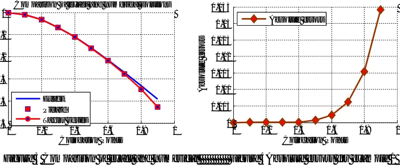
Figure 1Comparison of exact and numerical Figure 2 indicate the absolute errors for Example 1 solutions of Example 1.

Figure1 and Figure2 shows the comparison of exact and numerical solutions of Example 1 for

= = 1/2 (Taking first six terms for Picard’s and Taylor’s series method).

Case II:

For = , = 1, Equation (6) becomes

+ 3 =−2 , (11)

with initial condition (0) = 0. The exact solution of such problem is

0 0.2 0.4 0.6 0.8 1

0 0.2 0.4 0.6 0.8

1x 10

-4 Collocation Points A b s o lu te e rr o r Absolute error

0 0.2 0.4 0.6 0.8 1

-0.35 -0.3 -0.25 -0.2 -0.15 -0.1 -0.05 0 Collocation Points N u m e ri c a l S o lu ti o n s

Comparison of exact and numerical solutions

(7)

( ) =2

9(1− )−

2 3

For Picard’s Iterative Method:

=− ,

=− + ,

= − + −3

4 ,

=− + −3

4 +

9

20 ,

= − + −3

4 +

9

20 −

27

120 ,

……….

For Taylor Series Method:

=−2 −3 ⟹ (0) =−3 (0) = 0,

=−2−3 ⟹ (0) = −2−3 (0) =−2,

= −3 ⟹ (0) = −3 (0) = 6,

= −3 ⟹ (0) = −3 (0) =−18,

………

Taylor series expansion is

( ) = (0) + (0) +

2 (0) + 6 (0) +24 ′(0) +− − − −

( ) =− + −3

4 +

9

20 −

27

(8)

Figure 3 Comparison of exact and numerical Figure 4Absolute errors for example 1

solutions of Example 1(Case II) (Case II)

Figure3 and Figure4 shows the comparison of exact and numerical solutions of Example

1for = , = 1 (Taking first six terms for Picard’s and Taylor’s series method).

ATMOSPHERIC PRESSURE:

To find the atmospheric pressure . . at a height . above the sea level, when the

temperature is constant.

Let a vertical column of air of unit cross-section. Let be the pressure at a height above the

sea-level and + at height + . Let be the density at a height . Since the thin column of air is

being pressured upwards with pressure and downwards with pressure + . By considering

equilibrium, we get

= + + (12)

From (12), we get

=− , (13)

which is the differential equation giving the atmospheric pressure at a height .

When the temperature is constant, = using Boyle’s law, we get

= − , (14)

with initial condition (0) = . The exact solution is

= .

Letting = 1.

0 0.2 0.4 0.6 0.8 1

-0.5 -0.4 -0.3 -0.2 -0.1 0 Collocation Points N u m e ri c a l S o lu ti o n s Exact Picard Taylor series

0 0.2 0.4 0.6 0.8 1

(9)

For Picard’s Iterative Method:

= 1− ,

= 1− + 1

2! ,

= 1− + 1

2! −

1

3! ,

= 1− + 1

2! −

1

3! +

1

4! ,

………

For Taylor series method:

=− , ′(0) =− ,

′ = − , ′′(0) = ,

′′ =− , ′′′(0) =− ,

′′ =− , ′′′′(0) = ,

……….

Using Taylor’s series method,

( ) = (0) + (0) +

2! (0) +3! (0) + 4! (0)− − − − −

( ) = 1− +

2! −3! + 4! − − − − − −

CONCLUSION:

Picard’s and Taylor’s series methods are powerful mathematical tools for solving linear and

nonlinear differential equations. It is concluded that Picard’s and Taylor’s series methods gives more

accurate solutions, which are much closer to exact solutions, for solving first order differential

equations arising in some applications of sciences and engineering.

REFERENCES

1. RevathiG. Numerical solutions of ordinary differential equations and applications.

International Journal of Management and Applied Sciences. 2017;3(2):1-5.

2. Yang XH, Liu YJ. Picard iterative process for initial value problems of singular fractional

(10)

problems.Appl. Math. Lett. 2004;17:1231-1237.

4. Lakshmikantham V, Vatsala AS. Basic theory of fractional differential equations. Nonlinear

Anal. 2008; 69: 2677–2682.

5. Harier E, Norsett SP, Wanner G. Solving ordinary differential equations, II. Stiff and

Differential-Algebraic Problems. Springer Verlag; 1991.

6. Newton I. Methodus Fluxionum et Serierum In finatarum. Edita Londini 1736. Opuscula

Mathematica I;1761.

7. Euler L. Institutionum Calculi Integralis. Volumen Primum. Opera Omnia. XI; 1768.

8. Liouville J. Sur le developement des fonctionsou parties de fonctionsen series don’t les divers

termessontassujetis a satisfaire a une meme equation differentielle du second ordre,

contenatuneparametre variable. Journal De Math. Pures et appl.1836;1: 253-265.

9. PeanoG. Integration par series des ´equations differentielleslin´eaires. Math. Annallen.1888;

32: 450-456.

10.Picard. Memoire sur la theorie des équations aux dériveespartiellee et la méthode des

approximations successive.J. de Math. Pures et appl. 4e s´erie.1899; 6: 145-210.

11.Hirayama H. Numerical technique for solving an ordinary differential equation by Picard’s

method. Integral Methods in Science and Engineering. 2002: 111-116.

12. Corliss G, Chang YF. Solving ordinary differential equations using Taylor series.A.C.M.