Multi-Mode Resource-Constrained
Project-Scheduling Problem With Renewable
Resources: New Solution Approaches
Selcuk Colak, Cukurova University, Turkey Anurag Agarwal, University of South Florida, USA
Selcuk Erenguc, University of Florida, USA
ABSTRACT
We consider the multi-mode resource-constrained project scheduling problem (MRCPSP) with renewable resources. In MRCPSP, an activity can be executed in one of many possible modes; each mode having different resource requirements and accordingly different activity durations. We assume that all resources are renewable from period to period, such as labor and machines. A solution to this problem basically involves two decisions – (i) The start time for each activity and (ii) the mode for each activity. Given the NP-Hard nature of the problem, heuristics and metaheuristics are used to solve larger instances of this problem. A heuristic for this type of problem involves a combination of two priority rules - one for each of the two decisions. Heuristics generally tend to be greedy in nature. In this study we propose two non-greedy heuristics for mode selection which perform better than greedy heuristics. In addition, we study the effect of double justification and backward/forward scheduling for the MRCPS. We also study the effect of serial vs. parallel scheduling. We found that all these elements improved the solution quality. Finally we propose an adaptive metaheuristic procedure based on neural networks which further improves the solution quality. The effectiveness of these proposed approaches, compared to existing approaches in the literature, is demonstrated through empirical testing on two well-known sets of benchmark problems.
Keywords: Project Management; Scheduling; Heuristics; Metaheuristics; Multi-Mode Resource-Constrained Project-Scheduling
1. INTRODUCTION
anaging projects efficiently and effectively is critical to organizational success in today’s highly competitive business environment. We study the multi-mode resource-constrained project-scheduling problem (MRCPSP) which is a generalization of the classical resource-constrained project-scheduling problem (RCPSP). In RCPSP, activities of a project follow some precedence constraints and are processed in some predetermined duration of time using some predetermined amounts of resources. Resources are assumed to be limited for each period. The activities can be scheduled as they become resource and precedence feasible. The objective is to minimize the project completion time or makespan. The generalization of RCPSP occurs on two dimensions - first, in MRCPSP, each activity can be processed in multiple modes. A mode implies a certain level of resources used. The activity durations vary with the levels of resources used. Allocating more (or better quality) resources can accelerate activity duration. For example, an activity which takes two days to complete with three workers (mode 1) may be completed in only one day with six workers of the same skill level (mode 2) or with four workers of a higher skill level (mode 3). The second generalization has to do with the nature of resources. In MRCPSP, three types of resources are considered – renewable, non-renewable and doubly constrained (Slowinski, 1980). Renewable resources are available in limited quantities for each time period and are renewable from period to period (e.g. labor, machines). Non-renewable resources are limited for the entire project (e.g. project budget). Doubly-constrained resources are limited both for the entire project as well as for each period.
The first generalization, the one that allows use of different levels of resources to be allocated to activities, makes the MRCPSP of much greater practical significance to the project manager than the single-mode version of the problem, the RCPSP. This is because in the real world, managers generally enjoy the prerogative of manipulating resource levels in order to accelerate critical activities to reduce the overall project duration. Yet, the MRCPSP is not as widely studied as the RCPSP. As far as the second generalization, which takes into account renewable, non-renewable and doubly-constrained resources, the renewable resource problem is most commonly found in practice because most resources are procured in markets through funding. Of course, if funding is limited, then all resources become non-renewable.
To the best of our knowledge, while the most general MRCPSP problem has received wide attention, the problem of only renewable resources has received very little attention in the literature. The only studies, to the best of our knowledge, on MRCPSP with only renewable resources are by Boctor (1993, 1996a and 1996b), Mori and Tseng (1997) and Alcaraz et al. (2003). Further, of the 19 sets of benchmark MRCPSP instances in PSPLIB, only one set is devoted to only renewable resources. Boctor (1993) has also developed a set of benchmark problems for the MRCPSP problems with renewable-only resources. Given the practical significance of this problem, there is a need to explore better solution approaches. In this paper, we develop new solution approaches for solving the MRCPSP with renewable resources only, hereafter MRCPSP-RR. The objective is to determine the execution mode and the start time of each activity in order to minimize the project completion time or the makespan, while satisfying the precedence and resource constraints. Activities are assumed to be non-preemptive, a common assumption in the literature. The MRCPSP-RR is a strongly NP-Hard problem as it is a generalization of the RCPSP which itself is strongly NP-Hard.
Formally, the MRCPSP-RR can be described as follows: A project consists of N activities represented by index i = 1, …, N. The Nth activity is the dummy terminal activity with no successors and a duration of zero. Each activity can be executed in one of j modes, where j goes from 1 to Mi, where Mi is the number of possible modes for
activity i. Once a mode has been selected for an activity, it must be finished without switching the mode. The duration of activity i executed in mode j is dij. The non-preemptive assumption implies that once an activity i has
been assigned mode j, it must be executed for dij consecutive time units without interruption. Activity icannot start
before all of its predecessors have been completed. We assume there are Rkt amount of renewable resources of type
k available in time period t. Index k goes from 1 to K, where K is the total number of resource types. Activity i executed in mode jrequires rijkresource units per period for resource type k. The activity durations, resource
availabilities and resource requirements per activity are non-negative integers. Further assume that Ei is the earliest
finish time and Li the latest finish time of activity i. Ei is calculated using a forward pass of the PERT chart using
the critical path method assigning the fastest mode to each activity. LN is then set equal to an upper bound T where
T is the sum of activity durations of all activities with the slowest execution modes. Li for the rest of the activities
are calculated using a backward pass of the PERT chart assuming the slowest resource mode is assigned to activities. Also let Pi be the set of all preceding activities of activity i. We also define xijt as a 0-1 binary variable
which assumes a value of 1 if activity i is assigned to mode j having a finish time of t and zero otherwise. The integer programming formulation of the problem is described as:
Minimize:
.
.N
N
L
N t t E
t x
Subject to:
1
1
1,...,
i i
i
M L
ijt j t E
x
i
N
(1)1 1
.
(
).
1,...,
,
p p i i
p i
M L M L
ijt ij ijt i
j t E j t E
t x
t
d
x
i
N p
P
1
1 1
.
1,...,
,
1,...,
ij i t d
M N
ijk ijs kt i j s t
r x
R
k
K t
T
(3)Constraint set (1) ensures that each activity is executed only once, set (2) ensures that the precedence constraints are satisfied and set (3) ensures that the resource constraints are satisfied. For large N the problem is difficult to solve optimally and therefore heuristics are used.
In solving this problem heuristically, two decisions are involved – (i) which activity to be assigned if two or more activities are precedence and resource feasible and (ii) which of the several feasible modes of execution to select for the assigned activity. Two priority rules are therefore needed to solve the problem - one for activity selection and one for execution-mode selection. These two priority rules working in tandem constitute a heuristic for solving this type of problem. If we considered x number of rules for activity selection, and y for mode selection, then the total number of rule combinations (heuristics) for the MRCPSP with renewable resources would be x * y. In this paper, we (i) two non-greedy heuristics (priority rules) for mode selection and a new greedy rule for activity selection, (ii) study the effect of double justification, (iii) study the effect of forward/backward scheduling, (iv) study the effect of serial vs. parallel scheduling and (v) propose an adaptive metaheuristic, based on neural network principles, to solve the problem iteratively using weighted activity-durations. While the effect of double justification and serial vs. parallel scheduling have been studied for the RCPSP, they have not been studied for the MRCPSP.
In the next section (Section 2), we review the relevant literature for the general MRCPSP as well as the MRCPSP with only renewable resources. Section 3 describes the existing heuristics in the literature and also the new heuristics developed in this study. The proposed adaptive metaheuristic is detailed in Section 4. In Section 5 we present the results of our computational experiments and compare our results with those of previous approaches in the literature. Summary and concluding remarks appear in Section 6.
2. RELEVANT LITERATURE
The MRCPSP was first introduced by Elmaghraby (1977). Talbot (1982) was the first to propose an exact solution method using the implicit enumeration scheme. Patterson et al. (1989, 1990) presented a more powerful backtracking procedure for solving the problem. These approaches, however, were unable to solve instances with more than 15 activities in reasonable computation time. Demeulemeester and Herroelen (1992) had proposed a branch-and-bound procedure for the RCPSP, which was extended to the MRCPSP by Sprecher et al. (1997). Hartman and Drexl (1998) compared the existing branch-and-bound algorithms and presented an alternative exact approach based on the concepts of mode and extension alternatives. Sprecher and Drexl (1998) proposed an exact solution procedure by extending the precedence-tree guided enumeration scheme of Patterson et al. (1989, 1990). Although their approach was the most powerful procedure, it was unable to solve the highly resource-constrained problems (more than 20 activities and two modes per activity) in reasonable computational times.
Several heuristics and metaheuristics have also been proposed in the literature for this problem. Drexl and Grunewald (1993) presented a stochastic scheduling method. Ozdamar and Ulusoy (1994) proposed a local constraint based approach that selects the activities and their respective modes locally at every decision point. Kolisch and Drexl (1997) developed a local search method that first finds a feasible solution and then performs a neighborhood search on the set of feasible mode assignments. Different genetic algorithms for solving the MRCPSP have been developed by Mori and Tseng (1997), Ozdamar (1999), Hartmann (2001) and Alcaraz et al. (2003). Simulated annealing algorithms are one of the most common heuristic procedures applied to MRCPSP. Slowinski et al. (1994), Bouleimen and Lecocq (2003) and Jozefowska et al. (2001) have suggested simulated annealing algorithms. Nonobe and Ibaraki (2002) proposed a tabu-search procedure for this problem. More recently, Lova et al, (2009) have proposed a hybrid genetic algorithm and Barrios et al. (2011) have proposed a Double genetic algorithm for this problem.
Details of these rules are presented in the next section. In a follow-up study, Boctor (1996a) proposed backward/forward scheduling to improve the results and also proposed a new priority rule for mode selection. The new rule, although very complex, gave better results. Boctor (1996b) proposed a simulated annealing approach and Alcaraz et al. (2003) proposed a genetic algorithm approach for this problem. Both simulated annealing and genetic algorithms improved the results from single-pass heuristics significantly.
In the next section, we will briefly describe the heuristics that have been used to solve MRCPSP problem and explain our proposed greedy and non-greedy heuristics.
3. HEURISTIC METHODS FOR MRCPSP-RR
3.1 Existing Heuristics
In the existing literature, parallel schedule generation scheme is used. In this scheme, a clock is maintained which is moved to a point when the next activity or activities become precedence-feasible and resource-feasible. Assignment takes place from amongst the activities that are ready for assignment, based on an activity priority rule. Note that for each precedence-feasible activity, not all execution modes may be feasible at a given time. Once an activity is selected, the mode-selection priority rule is applied to choose one of several feasible execution modes. Boctor (1993) used seven rules for prioritizing activities and three for prioritizing execution modes resulting in twenty one heuristics. The seven rules for prioritizing activities were minimum total slack (Min-SLK), minimum latest finish time (Min-LFT), maximum number of immediate successors (Max-NIS), maximum remaining work (Max-RWK), maximum processing time (Max-PTM), minimum processing time (Min-PTM) and maximum number of subsequent candidates (Max-CAN). Of these seven, Min-SLK, Max-RWK, Max-CAN and Min-LFT performed better than the other three. The three rules for prioritizing execution modes were: shortest feasible mode (SFM), least criticality ratio (LCR) and least resource proportion (LRP). Of these three, the SFM rule dominated the other two. So, the four best heuristics (or rule combinations) were Min-SLK/SFM, Max-RWK/SFM, Max-CAN/SFM and Min-LFT/SFM. Boctor, in a follow-up study (Boctor, 1996a), focused on these four heuristics and improved the results by solving twice: once forward and once backward and using the better of the two solutions. He also proposed a new rule for execution-mode selection, which we will call Boct96Rule, which gave better results than the SFM heuristic. This new rule attempted to prioritize execution modes based on certain conditions of non-dominated activity-mode combinations. Although complex to implement, this rule gave good results.
3.2 Proposed Heuristics
As far as the rules for prioritizing activities, we use the best of the seven rules proposed by Boctor (1993), namely Max-RWK. We propose a new heuristic called minimum latest start time (Min-LST). This rule has been used in many other types of scheduling problems, so it is not new to the scheduling literature, but is new for MRCPSP-RR and it gave better results than the other seven activity priority rules used in Boctor (1996a).
For prioritizing execution modes we propose two new, non-greedy approaches which take into account the criticality of an activity. The non-greedy approaches differ from existing greedy approaches in that, a precedence-feasible activity may not be scheduled in spite of being resource precedence-feasible for some execution mode. In the first non-greedy rule, if the feasible execution mode is not the fastest execution mode, we take into account the time the activity would have to wait for the resources for the fastest mode and the difference between the activity durations between the fastest mode and the fastest feasible mode. Clearly, if it has to wait less than the difference between the activity durations, it makes sense to wait. The waiting strategy is what makes the rule non-greedy.
In the second non-greedy rule, a precedence-feasible activity considers all modes faster than the fastest feasible mode and checks against each one the difference between the activity durations and the amount of waiting. If the fastest mode is not worth waiting for then perhaps the next fastest mode might be worth waiting. The first non-greedy rule, discussed earlier, would not wait for the second fastest mode but the second rule would.
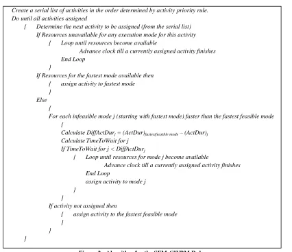
We call the first non-greedy rule for prioritizing execution mode the “Shortest Feasible Mode with Conditional Wait for the Fastest Mode” or SFM-CWFM, and the second rule “Shortest Feasible Mode with Conditional Wait for a Better Mode” or SFM-CWBM. We recommend taking the best of three mode selection rules – SFM, CWFM and CWBM. Figure 1 shows the pseudo-code of the proposed heuristic using SFM-CWFM rule and Figure 2 shows the same with the SFM-CWBM rule.
Create a serial list of activities in the order determined by activity priority rule. Do until all activities assigned
{ Determine the next activity to be assigned (from the serial list) If Resources unavailable for any execution mode for this activity
{ Loop until resources become available
Advance clock till a currently assigned activity finishes End Loop
}
If Resources for the fastest mode available then { assign activity to fastest mode
} Else
{ Calculate DiffActDur = (ActDur)fastestfeasible mode – (ActDur)fastest infeasiblemode
CalculateTimeToWait for the fastest mode If TimeToWait for fastest mode < DiffActDur
{ Loop until resources for fastest mode become available Advance clock till a currently assigned activity finishes End Loop
assign activity to fastest mode }
Else
{ assign activity to fastest feasible mode }
} }
Create a serial list of activities in the order determined by activity priority rule. Do until all activities assigned
{ Determine the next activity to be assigned (from the serial list) If Resources unavailable for any execution mode for this activity
{ Loop until resources become available
Advance clock till a currently assigned activity finishes End Loop
}
If Resources for the fastest mode available then { assign activity to fastest mode }
Else {
For each infeasible mode j (starting with fastest mode) faster than the fastest feasible mode {
Calculate DiffActDurj = (ActDur)fastestfeasible mode – (ActDur)j
CalculateTimeToWait for j If TimeToWait for j < DiffActDurj
{ Loop until resources for mode j become available
Advance clock till a currently assigned activity finishes End Loop
assign activity to mode j }
}
If activity not assigned then
{ assign activity to the fastest feasible mode }
} }
Figure 2: Algorithm for the SFM-CWBM Rule
We call this proposed approach ACE-SP (Agarwal, Colak and Erenguc – Single Pass). It consists of serial schedule generation scheme, better of backward and forward schedule and BFI or double justification and best of three mode selection rules. LST is basically ACE-SP with Min-LST activity priority rule and ACE-SP-RWK is ACE-SP with Max-ACE-SP-RWK activity priority rule. The next section describes the adaptive metaheuristic we use.
4. ADAPTIVE METAHEURISTIC
The adaptive metaheuristic is explained next, using the following notation:
k Iteration counter
kmax Max number of iterations
dij Activity duration of activity i executed in mode j.
wi Weight associated with the activity i.
wdij Weighted activity duration of activity i executed in mode j.
LSTi Latest start time of activity i.
RWKi Maximum remaining work for activity i.
MSk Makespan in the current iteration
MSB Best makespan Search coefficient WB Best weights
Step 1: Initialization
a. Initialize wi = 1, i = 1, …, N
b. Initialize the iteration counter k to 1. Step 2: Calculate weighted processing times
a. Calculate wdij = wi * dij , i = 1, …, N
Step 3: Determine priority list
a. Determine the priority list for the activities using a priority rule such as Min-LST or Max-RWK, where LST and RWK are calculated using wdij instead of dij.
Step 4: Determine makespan
a. Find a feasible schedule using serial schedule generation scheme, using the priority list. In other words, schedule each activity at its earliest possible time given precedence and resource constraints using one of the three mode selection priority rules (SFM, SFM-CWFM, SFM-CWBM). This schedule gives us the makespan msk.
Step 5: Apply search modification strategy and modify weights
a. If MSk is the best makespan so far, save the current weights as best weights (WB) and the makespan as
the best makespan (MSB).
b. If k = kmax, go to Step 7.
c. If k < kmax, modify the weights using the following strategy:
a. Generate a random number RND between 0 and 1 using uniform distribution.
i. If RND > 0.5 then (wi)k+1 = (wi)k + RND *
* errorii. If RND <= 0.5 then (wi)k+1 = (wi)k – RND *
* erroriii. error is the difference between the current makespan (MSk) and the lower bound (LB) for
the problem in question. Step 6: Next iteration
a. Increment k by one and go to step 2. Step 7: Display Solution
a. MSB is the solution. The schedule is generated using the WB.
The search coefficient () used in Step 5c determines the degree of weight change per iteration. A higher coefficient leads to a greater change and vice versa. One could therefore control the granularity of the search by varying . The search coefficient should neither be too low nor too high. A low will slow down convergence and make it difficult to jump local minima, while a high will render the search too erratic or volatile to afford convergence. With some empirical trial and error, we found that a rate of 0.005 worked well for all the problems.
5. COMPUTATIONAL EXPERIMENTS AND RESULTS
effectiveness of their proposed approaches. These problems were generated randomly and are divided into two main subsets - 120 instances of fifty-activities and 120 of one hundred-activities. In each subset, there are 40 instances each with respectively 1, 2 and 4 resource types. The average number of immediate successors is 2 and the number of execution modes for each activity is uniformly generated from 1 to 4.
The PSPLIB benchmark problems are mainly for the general MRCPSP. There are 19 sets of problems, each set having roughly 400 to 600 problems. One of the 19 sets of problems (set n0.mm) has instances with only renewable resources. There are 470 problems in this set. Results on these 470 problems using other approaches are not available explicitly in the literature.
Our heuristics were coded in Visual Basic .Net running on Windows-XP® operating system and implemented on a Pentium-4 PC.
5.1 Results for Boctor’s Benchmark Problems
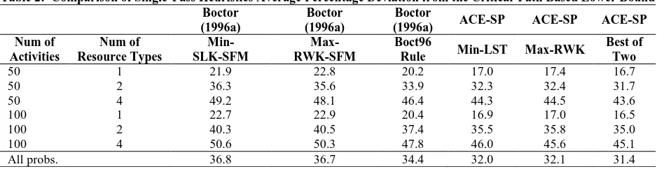
Results for the Boctor’s benchmark problems are presented now. Table 1 shows the average percent deviation from the critical-path based lower bound for the six single-pass heuristic combinations Min-LST-SFM, Min-LST-SFM-CWFM, Min-LST-SFM-CWBM, SFM, Max_RWK-SFM-CWFM and Max-RWK-SFM-SWBM. The lower bound is calculated using the shortest mode for each activity and assuming infinite resources.
Table 1: Comparison of Proposed Single-Pass Greedy and Non-Greedy Heuristics Average Percentage Deviation from the Critical-Path Based Lower Bound
Table 2 provides a comparison of these results with Boctor’s results on the average percent deviation measure. When we take the best of six heuristics, the average gap for all problems is 31.4 percent compared to Boctor’s best results of 34.4 percent. Even individually, the average gaps for the six heuristics range from 32.00 to 33.23, all being better than the 34.4 percent.
Table 2: Comparison of Single-Pass Heuristics Average Percentage Deviation from the Critical-Path Based Lower Bound Boctor
(1996a)
Boctor (1996a)
Boctor
(1996a) ACE-SP ACE-SP ACE-SP
Num of Activities Num of Resource Types Min- SLK-SFM Max- RWK-SFM Boct96
Rule Min-LST Max-RWK
Best of Two
50 1 21.9 22.8 20.2 17.0 17.4 16.7
50 2 36.3 35.6 33.9 32.3 32.4 31.7
50 4 49.2 48.1 46.4 44.3 44.5 43.6
100 1 22.7 22.9 20.4 16.9 17.0 16.5
100 2 40.3 40.5 37.4 35.5 35.8 35.0
100 4 50.6 50.3 47.8 46.0 45.6 45.1
All probs. 36.8 36.7 34.4 32.0 32.1 31.4
Num of Activities Num of Resource Types Min- LST- SFM Min- LST- SFM- CWFM Min- LST- SFM- CWBM Min- LST Best of Three Max- RWK- SFM Max- RWK- SFM- CWFM Max- RWK- SFM- CWBM Max- RWK Best of Three
50 1 18.46 17.81 17.86 16.99 18.66 18.19 18.19 17.44
50 2 33.50 33.85 33.68 32.32 33.59 33.94 33.75 32.36
50 4 45.08 45.79 45.87 44.31 45.38 45.72 45.79 44.48
100 1 18.31 17.25 17.27 16.91 18.15 17.38 17.35 16.95
100 2 36.68 36.23 36.23 35.50 37.05 36.29 36.29 35.84
100 4 47.38 46.39 46.39 45.96 47.02 46.07 46.04 45.65
Table 3: Comparison of Single-Pass Heuristics Maximum Deviation from the Critical-Path Based Lower Bound Boctor (1996a) Boctor (1996a) Boctor
(1996a) ACE-SP ACE-SP
Num of Activities Num of Resource Types Min- SLK-SFM Max- RWK-SFM Boct96 Rule Min- LST Max- RWK
50 1 35.9 41.8 30.4 28.0 29.1
50 2 50.5 52.6 46.0 48.8 47.3
50 4 67.9 59.8 60.3 57.8 57.4
100 1 33.4 34.3 31.1 25.9 27.1
100 2 55.0 54.3 48.5 52.4 53.3
100 4 66.7 69.3 60.2 59.0 58.2
All probs. 67.9 69.3 60.3 59.0 58.2
Table 4: Comparison of Single-Pass Heuristics Minimum Deviation from the Critical-Path Based Lower Bound Boctor
(1996a)
Boctor (1996a)
Boctor
(1996a) ACE-SP ACE-SP
Num of Activities Num of Resource Types Min- SLK-SFM Max- RWK-SFM Boct96 Rule Min- LST Max- RWK
50 1 10.9 8.9 11.3 5.7 7.2
50 2 22.5 18.2 18.8 17.3 18.6
50 4 35.6 35.6 32.8 32.3 31.9
100 1 14.1 14.9 12.8 8.6 8.2
100 2 28.0 27.4 27.4 21.4 23.5
100 4 41.2 41.3 39.7 37.9 37.0
All probs. 10.9 8.9 11.3 5.7 7.2
Tables 3 and 4 compare the ACE heuristics with Boctor’s results on two other measures - maximum and minimum deviations from the lower bound. The maximum deviations for the two ACE-SP heuristics are 59% and 58.2% compared to 60.3% obtained by Boctor96 rule. The minimum deviations are 5.7% and 7.2% compared to 11.3% of Boctor96 rule.
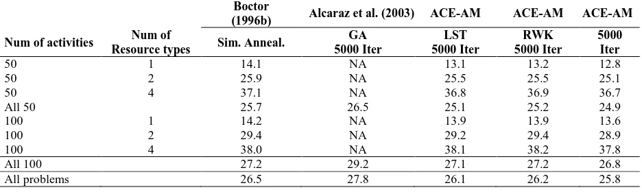
The results of the adaptive metaheuristic (ACE-AM) are now explained. For the adaptive metaheuristic, the search coefficient was set to 0.005 and the weights were initialized at 1. The determination of the best value of the search coefficient required some trial and error on a small set of problems. We report results for solutions obtained using 5,000 iterations. Average CPU times of our adaptive metaheuristic with Min-LST were 6.7 seconds for 5,000 iterations. The evaluation criterion we use is the average percentage deviation from the critical-path-based lower bound. Table 5 shows the results of ACE-AM for LST and RWK heuristics for 5,000 iterations. The results of this study are compared with those of the simulated-annealing approach of Boctor (1996b) and genetic algorithm approach of Alcaraz et al. (2003). For the entire set of 240 problems, the best of LST and ACE-AM-RWK gives a deviation of 25.8% from the lower bound while the same deviations using simulated annealing and genetic algorithms were 26.5% and 27.8%, respectively. Even without considering the best of Min-LST and Max-RWK, each of the proposed approaches outperforms the existing approaches.
Table 5: Comparison of Metaheuristics Average Percentage Deviation from the Critical-Path Based Lower Bound Boctor
(1996b) Alcaraz et al. (2003) ACE-AM ACE-AM ACE-AM
Num of activities Num of
Resource types Sim. Anneal.
GA 5000 Iter LST 5000 Iter RWK 5000 Iter 5000 Iter
50 1 14.1 NA 13.1 13.2 12.8
50 2 25.9 NA 25.5 25.5 25.1
50 4 37.1 NA 36.8 36.9 36.7
All 50 25.7 26.5 25.1 25.2 24.9
100 1 14.2 NA 13.9 13.9 13.6
100 2 29.4 NA 29.2 29.4 28.9
100 4 38.0 NA 38.1 38.2 37.8
All 100 27.2 29.2 27.1 27.2 26.8
5.2 Results for PSPLIB Problems
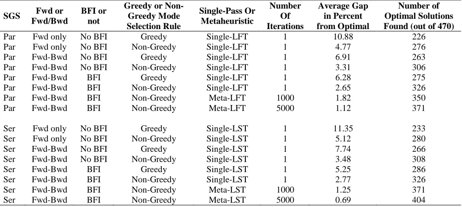
There are 470 problems in the n0.mm dataset of the PSPLIB benchmark problems for MRCPSP. Results for these 470 problems do not appear explicitly in the literature. Optimum solutions using exact approaches are known. The number of activities in these problems range from 12 to 22. So they are not quite as large as Boctor’s problems and are therefore solvable optimally using exact methods. We provide the gaps from the optimal solutions and also show how many of the 470 problems were solved to optimality. Table 6 shows the results of using Parallel and Serial SGS, with various combinations of forward/backward and BFI and Mode selection heuristics.
Table 6: Average Gap from Optimal and Number of Problems Solved to Optimality for PSPLIB n0.mm Dataset Using Various Procedures
SGS Fwd or
Fwd/Bwd
BFI or not
Greedy or Non-Greedy Mode Selection Rule
Single-Pass Or Metaheuristic
Number Of Iterations
Average Gap in Percent from Optimal
Number of Optimal Solutions Found (out of 470)
Par Fwd only No BFI Greedy Single-LFT 1 10.88 226
Par Fwd only No BFI Non-Greedy Single-LFT 1 4.77 276
Par Fwd-Bwd No BFI Greedy Single-LFT 1 6.91 263
Par Fwd-Bwd No BFI Non-Greedy Single-LFT 1 3.31 306
Par Fwd-Bwd BFI Greedy Single-LFT 1 6.28 275
Par Fwd-Bwd BFI Non-Greedy Single-LFT 1 2.65 326
Par Fwd-Bwd BFI Non-Greedy Meta-LFT 1000 1.82 350
Par Fwd-Bwd BFI Non-Greedy Meta-LFT 5000 1.12 371
Ser Fwd only No BFI Greedy Single-LST 1 11.35 233
Ser Fwd only No BFI Non-Greedy Single-LST 1 5.12 280
Ser Fwd-Bwd No BFI Greedy Single-LST 1 7.74 266
Ser Fwd-Bwd No BFI Non-Greedy Single-LST 1 3.48 308
Ser Fwd-Bwd BFI Greedy Single-LST 1 5.25 286
Ser Fwd-Bwd BFI Non-Greedy Single-LST 1 2.77 326
Ser Fwd-Bwd BFI Non-Greedy Meta-LST 1000 1.25 371
Ser Fwd-Bwd BFI Non-Greedy Meta-LST 5000 0.69 404
Although for single-pass, parallel SGS performed marginally better than serial SGS. For example, parallel SGS for single pass gave a 2.65 percent gap vs. a 2.77 percent gap by serial SGS. For the adaptive metaheuristic, Serial SGS gave much superior results. For 5000 iterations, serial SGS gave an average gap of only 0.69 percent compared to a gap of 1.12 percent for parallel SGS. Introduction of Non-Greedy rule for model selection resulted in significant improvement. For example, for parallel SGS, for forward only and no BFI procedure, the gap reduced from 10.88 percent to 4.77 percent. For serial SGS, the non-greedy procedure helped reduce the gap from 11.35 percent down to 5.12 percent. Use of Forward-Backward scheduling also resulted in significant improvements. For example, for parallel SGS, the gap reduced from 10.88 percent to 6.91 percent by applying forward-backward procedure. Use of BFI resulted in marginal improvements. For example, for parallel SGS, use of BFI reduced the gap from 6.91 percent down to 6.28 percent. Of course, the use of adaptive metaheuristic further improved the results. The improvement owing to metaheuristics is particularly remarkable with the Serial SGS (from 2.77 down to 0.69 percent) compared to Parallel SGS (from 2.65 percent to 1.12 percent). The average CPU time for the single-pass heuristics were 0.0002 seconds. For the metaheuristics, for 1000 iterations it was 0.181 seconds and for 5000 iterations it was 0.821 seconds.
6. SUMMARY AND CONCLUSIONS
which, a precedence-feasible activity may not be scheduled in spite of being resource feasible for at least one execution mode and waits for the fastest mode or one of the faster modes if the wait is worth it. These rules are called shortest feasible mode with conditional wait for fastest mode (SFM-CWFM) and shortest feasible mode with conditional wait for better mode (SFM-CWBM). We also proposed an adaptive metaheuristic, in which we use weighted activity-durations instead of given activity durations. A single-pass heuristic is applied iteratively to the problem using weighted activity-durations. The weights, which are the same for all activities for the first iteration, are modified at the end of each iteration. We also studied the effect of applying serial schedule generation scheme and found that it gave better results than parallel schedule generation scheme. Backward forward scheduling and double justification schemes were also applied, each of which provided some improvement.
The proposed algorithms were tested on two sets of benchmark problems from the literature. The results demonstrated that for Boctor’s benchmark problems, the non-greedy rules for mode selection were slightly better than their greedy counterparts, the proposed greedy rule for activity selection performed slightly better than previously proposed rules and the adaptive metaheuristic outperformed the simulated annealing algorithm of Boctor (1996b) and genetic algorithm of Alcaraz et al. (2003). The gaps between the obtained solution and the critical path based lower bound using the proposed approaches was about 10% lower than the competitive approaches in the literature. Each element of the proposed approach contributed a little towards the reduction in the gap. For the PSPLIB benchmark problems, our approach was within 1.5% of the optimal, with 374 problems solved to optimality using 1000 iterations.
From the managerial perspective, such significant reductions in the makespan can amount to huge cost savings for the project. In a competitive business environment in which project completion deadlines are strictly imposed and penalties for missing the deadlines can be high, generating a better schedule can help avert those penalties. In competitive bidding environment, organizations can bid lower to win contracts.
We encourage more future research in this area. To many project managers a criterion other than makespan minimization might be of more interest. To some, a multi-criteria objective may be important. Heuristics and metaheuristics for these different objectives need to be developed for this problem.
AUTHOR INFORMATION
Selcuk Colak is an Associate Professor in the Department of Business at the Cukurova University, Adana, Turkey. His current research interests are: heuristics and metaheuristics, genetic algorithms, neural networks, project and machine scheduling, distribution planning. Professor Colak teaches Operations Management, Project Management and Logistics Management courses both undergraduate and graduate level. Selcuk Colak received his B.S. in Electrical and Electronics Engineering in 1997 from the Cukurova University in Adana, Turkey. He received his M.S. in Electrical and Computer Engineering in 2000 and his Ph.D. in Information Systems and Operations Management in 2006 from the University of Florida, Gainesvlle, FL, USA. E-mail: scolak@cu.edu.tu
Dr. Anurag Agarwal is a Professor in the Department of Information Systems and Decision Sciences at University of South Florida, Sarasota, FL, USA. He earned his Ph.D. from The Ohio State University, Columbus, OH, USA (1993) and an MBA from the University of Wisconsin, La Crosse, WI, USA (1988). He teaches a variety of courses in Information Systems, Statistics and Operations Management, both at the undergraduate and graduate levels. His primary research interests are in heuristics and metaheuristics for various optimization problems. E-mail: agarwala@sar.usf.edu (Corresponding author)
REFERENCES
1. Agarwal, A., Colak, S. and Eryarsoy, E. (2006). Improvement Heuristic for the Flow-Shop Scheduling Problem: An Adaptive-Learning Approach. European Journal of Operational Research. 169(3): 801-815. 2. Alcaraz, J., Maroto, C. and Ruiz, R. (2003). Solving the Multi-Mode Resource-Constrained Project
Scheduling Problem with genetic algorithms. Journal of the Operational Research Society.54(6): 614-626. 3. Barrios, A., Ballestin, F. and Valls, V. (2011). A double genetic algorithm for the mrcpsp/max. Computers
& Operations Research. 38(1): 33-43.
4. Boctor, F.F. (1993). Heuristics for scheduling projects with resource restrictions and several resource-duration modes. International Journal of Production Research. 31(11): 2547-2558.
5. Boctor, F.F. (1996a). A new and efficient heuristic for scheduling projects with resource restrictions and multiple execution modes. European Journal of Operational Research,90(2): 349-361.
6. Boctor, F.F. (1996b). Resource Constrained Project Scheduling by simulated Annealing. International Journal of Production Research.34(8): 2335–2351.
7. Boulemein, K. and Lecocq, H. (2003). A new efficient simulated annealing algorithm for the resource-constrained project scheduling problem and its multiple-mode version. European Journal of Operational Research. 149(2): 268-281.
8. Demeulemeester, E. and Herroelen, W. (1992). A branch-and-bound procedure for the multiple resource constrained project scheduling problem. Management Science.38(12): 1803-1818.
9. Drexl, A. and Grunewald, J. (1993). Nonpreemptive multi-mode resource-constrained project scheduling. IIE Transactions.25(5): 74-81.
10. Elmaghraby, S.E. (1977). Activity Networks: Project Planning and Control by Network Models. Wiley, New York, 1977.
11. Hartmann, S. and Drexl, A. (1998). Project scheduling with multiple modes: a comparison of exact algorithms. Networks. 32(4): 283–297.
12. Hartmann, S. (2001). Project scheduling with multiple modes: a genetic algorithm. Annals of Operational Research. 102(1): 111–135.
13. Jozefowska, J., Mika, M., Rozycki, R., Waligora, G. and Weglarz, J. (2001). Simulated annealing for multi-mode resource-constrained project scheduling. Annals of Operational Research,102(1): 137–155. 14. Kolisch, R., (1996). Serial and parallel resource-constrained project scheduling methods revisited.
European Journal of Operational Research. 90(2): 320-333.
15. Kolisch, R. and Drexl. A. (1997). Local search for non-preemptive multi-mode resource-constrained project scheduling. IIE Transactions.29(11): 987-999.
16. Kolisch, R. and Sprecher, A. (1997). PSPLIB --- a project scheduling problem library. European Journal of Operational Research. 96, 205-216.
17. Lova, A., Tormos, P., Cervantes, M, and Barber, F. (2009) An efficient hybrid genetic algorithm for scheduling projects with resource constraints and multiple execution modes. International Journal of Production Economics. 117(2): 302-316.
18. Mori, M. and Tseng, C.C. (1997). A genetic algorithm for multi-mode resource constrained project scheduling problem. European Journal of Operational Research. 100(1): 134–141.
19. Nonobe K. and Ibaraki, T. (2002) Formulation and tabu search algorithm for the resource constrained project scheduling problem. Essays and Surveys in Metaheuristics. Eds. Ribeiro and P. Hansen, Kluwer Academic Publishers.
20. Ozdamar, L. (1999). A genetic algorithm approach to a general category project scheduling problem. IEEE Transactions on Systems, Man, and Cybernetics Part C. 29(1): 44-59.
21. Ozdamar, L. and Ulusoy. G. (1994). A local constraint based analysis approach to project scheduling under general resource constraints. European Journal of Operational Research. 79(2): 287-298.
22. Patterson, J.H., Slowinski, R., Talbot, F.B. and Weglarz, J. (1989). An algorithm for a general class of precedence and resource constrained scheduling problem. Advances in Project Scheduling. Eds. Jan Weglarz and Joanna Jozefowska. Elsevier: Amsterdam. 3-28.
24. Slowinski R., Soniewicki, B. and Weglarz, J. (1994). DSS for multiobjective project scheduling. European Journal of Operational Research. 79(2): 220–229.
25. Sprecher, A. and Drexl, A. (1998). Multi-mode resource-constrained project scheduling by a simple, general and powerful sequencing algorithm. European Journal of Operational Research. 107(2): 431-450. 26. Sprecher, A., Hartmann, S. and Drexl, A. (1997). An exact algorithm for project scheduling with multiple
modes. OR Spektrum. 19, 195-203.
27. Talbot, F.B. (1982). Resource-constrained project scheduling with time-resource trade-offs: the non-preemptive case. Management Science. 28(10): 1197–1210.