Impact Factor (PIF): 2.365
Global Journal of Advance Engineering Technologies and Sciences
PERFORMANCE ANALYSIS OF FREQUENCY ESTIMATION USING
DIFFERENT ADAPTIVE FILTERS TECHNIQUES
Vinita Vaishnav
1,
Prof. Sunil Kumar Bhatt
2M. Tech. Scholar
1, Asst. Prof. & HOD
2Department of Electrical & Electronics Engineering
CENTRAL INDIA INSTITUTE OF TECHNOLOGY
,
INDORE (M.P.) India
ABSTRACT
The Electrical power system frequency is an important parameter. The frequency of operation is not constant but it varies depending upon the load conditions. In the operating, controlling and monitoring of electric devices power system parameters are having great contribution. So it is very important to accurately measure this slowly varying frequency. Under steady-state conditions the total power generated by power stations is equal to system load and losses. Frequency can deviate from its nominal value due to sudden appearance of generation-load mismatches. Frequency is a vital parameter which influences different relay functionality of power system.
In this paper study was made to estimate the frequency of measuring voltage or current signal in presence of random noise and distortion. Here we are first using linear techniques such as least mean square (LMS), algorithm for measuring the frequency from the distorted voltage signal. Then comparing these results with nonlinear techniques such as nonlinear least mean square (NLMS), and UNANR algorithms with different modulation techniques was Amplitude Modulation. Signal performance parameter PSNR measured and compared with respect to Signal to Noise Ratio. The performances of these algorithms are studied through MATLAB R2012a simulation.
I. INTRODUCTION
The whole dimension of communications has been changed by the rapid growth of technology. Today people are more interested in hands-free communication, which makes use of loud speaker and high gain microphone, in place of the old modeled wired telephone. The main advantage of wireless system is that, more than one person can participate in conversation while freely moving in the room. The presence of large acoustic coupling between speaker and microphone would produce a loud acoustic echo making the conversation difficult.
Frequency in electrical power system is an important operating parameter which is required to remain constant because it reflects the whole situation of the system. Frequency can show the active energy balance between generating power and load. Therefore frequency is considered as an index for operating power systems in practical. In power system frequency is not constant but changes according to load condition. Ideally this frequency should be constant, but due to noise, sudden appearance of load generation mismatches and increasing use of nonlinear load, the frequency of operating system is not constant. Component reactance change results due to deviation in system frequency from its desired value which influences different relay functionality of power system such as server damage or reactive power reduction occurs in system devices. So the frequency plays an essential role in operating, monitoring and controlling of any power system device.
A. Echo in Electrical System
The Echo is the phenomenon in which delayed and distorted version of an original sound or electrical signal is reflected back to the source. Two main characteristics of echo are reverberation and latency. Reverberation is the persistence of sound after stopping the original sound. This sound will slowly decay because of the absorption by the materials constructing the environment. Latency or delay is the different time of the signal between the transmitter and receiver. In the case of teleconference system, the sound is generated from loud speaker and received by microphone, the delay can compute base on the distance between them (i.e., the length of the direct sound). Delay = distance/speed of sound. There are two types of echo:
1. Electrical echo: caused by the impedance mismatch at the hybrids transformer which the subscriber two-wire lines are connected to telephone exchange four two-wire lines in the telecommunication systems.
Impact Factor (PIF): 2.365
unwanted noise signal. Silencers were important for noise cancellation over broad frequency range but expensive and not efficient at low frequencies.II. ADAPTIVE FILTERS
Digital signal processing (DSP) has been a major player in the current technical advancements such as noise filtering, system identification, voice prediction and echo cancellation. Standard DSP techniques, however, are not enough to solve these problems quickly and obtain acceptable results. Adaptive filtering techniques must be implemented to promote accurate solutions and a timely convergence to that solution. Adaptive Filter Adaptive filter is the most important component of acoustic noise canceller and it plays a key role in acoustic echo or noise cancellation. It performs the work of estimating the echo path of the room for getting a replica of echo signal. It requires an adaptive update to adapt to the environmental change. Another important thing is the convergence rate of the adaptive filter which measures that how fast the filter converges for best estimation of the room acoustic path. Adaptive filters are classified into two main groups: linear and nonlinear. Linear adaptive filters compute an estimate of a desired response by using a linear combination of the available set of observables applied to the input of the filter. Otherwise, the adaptive filter is said to be nonlinear.
A. Power system frequency estimation using LMS Algorithms
In 1959, Widow and Hoff derived an algorithm whose name was Least Mean Square (LMS) algorithm and till now it is one of the best adaptive filtering algorithms. This algorithm is used widely for different application such as channel equalization and echo cancellation. This algorithm adjusts the coefficients of (W)nof a filter in order to
reduce the mean square error between the desired signal and output of the filter. This algorithm is basically the type of adaptive filter known as stochastic gradient-based algorithms. Why it’s called stochastic gradient algorithm? Because in order to converge on the optimal Wiener solution, this algorithm use the gradient vector of the filter tap weights. This algorithm is also used due to its computational simplicity.
The LMS algorithm is a method to estimate gradient vector with instantaneous value. It changes the filter tap weights so that e(n) is minimized in the mean-square sense. The conventional LMS algorithm is a stochastic implementation of the steepest descent algorithm. It simply replaces the cost function ξ(n) = E[e2(n)] by its instantaneous coarse estimate.
Coefficient updating equation 1 for LMS is given by:
w(n + 1) = w(n) + μ i(n)e(n) 1
Where µ is a step-size parameter and it controls the immediate change of the updating factor. It shows a great impact on the performance of the LMS algorithm in order to change its value. If the value of µ is so small then the adaptive filter takes long time to converge on the optimal solution and in case of large value the adaptive filter will be diverge and become unstable.
B. Mathematical Derivation of the LMS algorithm
The derivation of LMS algorithm is the development of the steepest decent method and also takes help from the theory of Wiener solution (optimal filter tap weights). This algorithm is basically using the formulas which updates the filter coefficients by using the tap weight vectors w and also update the gradient of the cost function accordingly to the filter tap weight coefficient vector∇ξ(n). From Equation (2) in the steepest decent algorithm,
w(n + 1) = w(n) − μ∇ξ(n) 2
w(n + 1) = w(n) + μE{e(n)x(n)} 3
In practice, the value of the expectation E{e(n)x(n)} is normally unknown, therefore we need to introduces the approximation or estimated as the sample mean
Ě{e(n)x(n)} =1L∑L−1i=0e(n − l)x(n − l) 4
With this estimate we obtain the updating weight vector as, w(n − 1) = w(n) +µL∑L−1i=0 e(n − l)x(n − l)
Impact Factor (PIF): 2.365
If we using one point sample mean (L=1) then 𝐸̌{𝑒(𝑛)𝑥} = 𝑒(𝑛)𝑥(𝑛) 6And finally, the weight vector update equation become the simple form,
𝑤(𝑛 + 1) = 𝑤(𝑛) + 𝜇𝑒(𝑛)𝑥(𝑛) 7
C. Power system frequency estimation using Normalized LMS
Normalized Least Mean Square (NLMS) is actually derived from Least Mean Square (LMS) algorithm. The need to derive this NLMS algorithm is that the input signal power changes in time and due to this change the step-size between two adjacent coefficients of the filter will also change and also affect the convergence rate. Due to small signals this convergence rate will slow down and due to loud signals this convergence rate will increase and give an error. So to overcome this problem, try to adjust the step-size parameter with respect to the input signal power. Therefore the step-size parameter is said to be normalized.
It is another class of adaptive algorithm used to train the coefficients of the adaptive filter. This algorithm takes into account variation in the signal level at the filter output and selecting the normalized step size parameter that results in a stable as well as fast converging algorithm. The weight update relation for NLMS algorithm is as follows equation 8.
𝑤(𝑛 + 1) = 𝑤(𝑛) + 𝜇(𝑛) 𝑖(𝑛) 𝑒(𝑛) 8
By using this normalized step-size parameter in Least Mean Square algorithm, this algorithm is known as Normalized Least Mean Square (NLMS) algorithm. The step size for computing the update weight vector is, the variable step can be written as in equation 9.
𝜇(𝑛) =𝐶+‖𝑋(𝑛)‖𝛽 2 9
Where:
𝜇(𝑛) is step-size parameter at sample n 𝛽 is normalized step-size (0 < 𝛽 < 2) 𝐶 is safety factor (small positive constant).
The advantage of the NLMS algorithm is that the step size can be chosen independent of the input signal power and the number of tap weights. Hence the NLMS algorithm has a convergence rate and a steady state error better than LMS algorithm.
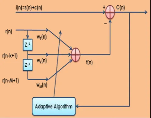
D. Adaptive Noise Reduction in UNANR algorithm
The UNANR model of the system performs the function of adaptive noise estimation. The UNANR model of order M, as shown in figure 1, is a transversal, linear, finite impulse response (FIR) filter. The response of the filter f(n) at each time instant (sample) n can be expressed as,
𝑓(𝑛) = ∑𝑀𝑚=1𝑊𝑚(𝑛)𝑟(𝑛 − 𝑚 + 1) 10
Where Wm (n) represents the UNANR coefficients, and r(n − m + 1) denotes the reference input noise at the
present (m = 1) and preceding m − 1, (1 < m ≤ M), input samples. In order to provide unit gain at DC, the UNANR coefficients should be normalized such that
∑Mm=1wm(n) = 1 11
The adaptation process of the UNANR model is designed to modify the coefficients that get convolved with the reference input in order to estimate the noise present in the given speech signal. To provide the estimated speech signal component, ŝ(n), at the time instant n, the output of the adaptive noise-reduction system subtracts the response of the UNANR model f(n) from the primary input i(n), i.e.,
𝑠̂(𝑛) = 𝑂(𝑛) = 𝑖(𝑛) − 𝑓(𝑛) 12
where the primary input includes the desired speech component and the additive white noise, i.e.,
Impact Factor (PIF): 2.365
Fig. 1: UNANR algorithm Model
Squaring both sides of yields:
𝑠̂2(𝑛) = 𝑖2(𝑛) + 𝑓2(𝑛) − 2𝑖(𝑛)𝑓(𝑛
= [𝑠(𝑛) + 𝑐(𝑛)]2+ 𝑓2(𝑛) − 2[𝑠(𝑛) + 𝑐(𝑛)]𝑓(𝑛)
= 𝑠2(𝑛) + 2𝑠(𝑛) 𝑢(𝑛) + 𝑢2(𝑛) + 𝑓2(𝑛) − 2[𝑠(𝑛) + 𝑐(𝑛)]𝑓(𝑛)
14
Different from the MMSE criterion, the goal of the UNANR coefficient adaptation process is considered to be the minimization of the instantaneous error ε(n) between the estimated signal power ŝ2(n) and the desired signal power s2(n), i.e.
ε(n) = ŝ2− s2(n) = c2(n) + 2s(n)c(n) + f2(n)2[s(n)c(n)]f(n)
15
Such a goal can be achieved by optimizing the UNANR coefficients according to the steepest-descent algorithm. The process of convergence in the multidimensional coefficient space follows a deterministic search path provided by the negative gradient direction as:
−∇wkε(n) = −
∂f2(n)
∂wk + 2
𝜕[𝑠(𝑛) + 𝑐(𝑛)]𝑓(𝑛) 𝜕𝑤𝑘
= −2𝑟(𝑛 − 𝑘 + 1) ∑𝑀𝑚=1𝑤𝑚(𝑛)𝑟(𝑛 − 𝑚 + 1) − 2𝑖(𝑛)𝑟(𝑛 − 𝑘 + 1)
= −2𝑟(𝑛 − 𝑘 + 1)[∑𝑀𝑚=1𝑤𝑚(𝑛)𝑟(𝑛 − 𝑚 + 1) − 𝑖(𝑛)] 16
By substituting into the standard steepest descent algorithm [13], we may derive the UNANR adaptation rule as
𝑤𝑘(𝑛 + 1) = 𝑤𝑘(𝑛) − 𝜂∇𝑤𝑘𝜀(𝑛)
= 𝑤𝑘(𝑛) − 2𝜂𝑟(𝑛 − 𝑘 + 1)[∑ 𝑤𝑚(𝑛)𝑟(𝑛 − 𝑚 + 1) − 𝑖(𝑛)] 𝑀
𝑚=1
= 𝑤𝑘(𝑛) + 2𝜂𝑟(𝑛 − 𝑘 + 1)[∑𝑀𝑚=1𝑤𝑚(𝑛)𝑟(𝑛 − 𝑚 + 1) 17
Impact Factor (PIF): 2.365
coefficients ŵ𝑘(𝑛 + 1) should be normalized so as to meet the requirement. The UNANR coefficient normalization formulation is given by:ŵk(n + 1) =∑ wkw(n+1)
k(n+1)
M
k=1 18
III. SIMULATION AND RESULTS
This project is all about the speech enhancement of voice signal using different adaptive filters. The speech signal is first mixed with a noise signal then it is modulated with two of the analog modulation techniques i.e. AM Then AWGN is chosen as a communication channel in configuration with one of the modulation technique. Then at the receiver side demodulation if performed and filtered with adaptive filters. The filters which are used are: LMS, NLMS and UNANR.
MATLAB is a numerical computing environment that especially effective to calculate and simulate the technical problems. This programming language is very powerful allows matrix manipulation, plotting of functions and data, implementation of algorithms, creation of user interfaces, and interfacing with other programming languages (C, C++, Fortran and Java). One of the most beneficial features is graphical visualization which helps us have confidence in results by monitoring and analyzing resultant plots. In addition, MATLAB implement Simulink, the software package models, simulates, and analyzes dynamic systems.
IV. PERFORMANCE OF AMPLITUDE MODULATION WITH AWGN CHANNEL
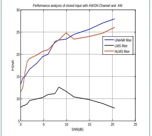
Consider the case of stored input speech signal first. In this case AM is selected to transmit the whole speech signal after addition of background noise at the transmitter side. AWGN channel is selected as a communication channel for transferring the speech signal. In AWGN channel, channel noise gets added to the speech signal. At the receiver side first AM demodulation is performed then speech signal is passed through one of the adaptive filter. Firstly LMS filter is selected and PSNR and RMSE signal parameters are -recoded. Secondly NLMS filter is selected for the same received demodulated speech signal.
0 0.5 1 1.5 2 2.5 3
x 104 -0.08
-0.06 -0.04 -0.02 0 0.02 0.04 0.06 0.08
original sinusoidal input signal
sample
A
m
p
lit
u
d
Impact Factor (PIF): 2.365
0 0.5 1 1.5 2 2.5 3
x 104 -0.2
-0.15 -0.1 -0.05 0 0.05 0.1 0.15
After modulation input signal
sample
A
m
p
lit
u
d
e
0 0.5 1 1.5 2 2.5 3
x 104 -0.4
-0.3 -0.2 -0.1 0 0.1 0.2 0.3
input signal with modulation and AWGN
sample
A
m
pl
itu
de
0 0.5 1 1.5 2 2.5 3
x 104 -0.1
-0.05 0 0.05 0.1 0.15
filtered signal output
sample
A
m
p
lit
u
d
Impact Factor (PIF): 2.365
Fig. 2 Offline Performance of Amplitude Modulation with AWGN channel , (a) Original stored sinusoidal signal, (b) After modulatedinput signal, (c) Input signal with modulation and AWGN, (d) Filtered signal output
Fig.3:Adaptive filtering on AM with AWGN channel for stored
V. PERFORMANCE OF FREQUENCY MODULATION WITH AWGN CHANNEL
In this case FM is selected to transmit the whole speech signal after addition of background noise at the transmitter side. AWGN channel is selected as a communication channel for transferring the speech signal. In AWGN channel, channel noise gets added to the speech signal. At the receiver side first FM demodulation is performed then speech signal is passed through one of the adaptive filter.
0 5 10 15 20 25
5 10 15 20 25 30
Performance analysis of stored input with AWGN Channel and AM
SNR(dB)
P
S
N
R
UNANR filter LMS filter NLMS filter
0 5 10 15 20 25 30 35
-30 -20 -10 0 10 20 30 40
Performance analysis of stored input with AWGN Channel
SNR(dB)
P
S
N
R
Impact Factor (PIF): 2.365
Fig. 4: Adaptive filtering on FM with AWGN channel for stored voiceVI. CONCLUSION
This Project work presented the adaptive algorithms (LMS, NLMS, UNANR) are implemented by using a sample input i.e. a stored voice and online voice signal and a wide band signal, additive white Gaussian noise. So noise canceller is implemented and the performance of different adaptive algorithms is compared.
Firstly LMS filter is selected and PSNR and RMSE signal parameters are recoded. Secondly NLMS filter is selected for the same received demodulated speech signal. And at the last UNANR filter is selected for the same received demodulated speech signal. Graphs have been plotted to check the performance of the adaptive filters. Graphs are plotted betweeSNR v/s PSNR. In the figure 4 for FM modulation technique with AWGN channel, performance of LMS, NLMS and UNANR are shown and graph is plotted between SNR and PSNR, Improvement after filtering with LMS, NLMS and UNANR algorithms with stored input sinusoidal signal with FM and AWGN.
REFERENCES
[1] B. L. Sim, et al., “A parametric formulation of the generalized spectral subtraction method”, IEEE Trans. on Speech and Audio Processing, vol. 6, pp. 328-337, 1998.
[2] M. Yasin et al. “Performance Analysis of LMS and NLMS Algorithms for a Smart Antenna System” International Journal of Computer Applications Vol.- 4. No.9, August 2010.
[3] I. Y. Soon, et al. “Noisy speech enhancement using discrete cosine transform”, Speech Communication, vol. 24, pp. 249-257, 1998.
[4] Md Zia Ur Rahman et al., “Filtering Non-Stationary Noise in Speech Signals using Computationally Efficient Unbiased and Normalized Algorithm” , International Journal on Computer Science and Engineering, Vol. 3 No. 3 Mar 2011.
[5] Sayed. A. et al. “A Family of Adaptive Filter Algorithms in Noise Cancellation for Speech Enhancement” International Journal of Computer and Electrical Engineering, Vol. 2, No. 2, April 2010.
[6] Priyanka Gupta et al. “Performance Analysis of Speech Enhancement Using LMS, NLMS and UNANR algorithms” IEEE 2015 (IC4_5230).
[7] B. Widrow, et al. “Adaptive noise cancelling: Principles and applications” , Proc. IEEE, vol. 63, pp.1692-1716, Dec. 1975.
[8]L. Stasionis, et al. “Selection of an Optimal Adaptive Filter for Speech Signal Noise Cancellation using C6455 DSP”, Electronics and Electrical Engineering. Kaunas: Technological, 2011.
[9] Md Zia Ur Rahman et al. “Filtering Non-Stationary Noise in Speech Signals using Computationally Efficient Unbiased and Normalized Algorithm” International Journal on Computer Science and Engineering (IJCSE), Vol. 3 No. 3 Mar 2011.
[10] Suleyman S. Kozat et al. “Unbiased Model Combinations for Adaptive Filtering”, IEEE Trans. on Signal Processing, Vol. 58, No. 8, August 2010.
[11] Anuradha R. Fukane et al. “Noise estimation Algorithms for Speech Enhancement in highly non-stationary Environments” IJCSI International Journal of Computer Science Issues, Vol. 8, Issue 2, March 2011.