Designed by intelligent fire detection system based on FFN and PMO using Sushisen algorithm analysis

International Journal of Advanced Trends in

Computer Applications

www.ijatca.com

Designed by intelligent fire detection system

based on FFN and PMO using Sushisen

algorithm analysis

1

Prof P. Senthil

MA, MSc, MPhil

1_{Associate professor in MCA Computer Science,}

Kurinji College of Arts and Science, Tiruchirappalli-620002.India.

1

[email protected]

Abstract:

optimization to find the fire time in the building. The use of intelligent methods in the fire detection system for data processing can reduce the risk of fire. In this paper, the original information of the firefighter network (FFN) is processed intelligently according to the possibility of the nervous system and the fire. In order to improve the quality of the system, the sensor data is applied to the generalized singular-value decomposition technique by analyzing the sound waves in the data. At the same time, the proposed neurological system was used for cell quality implantation new model particle mass optimization (PMO) using sushisen algorithms. In the simulation work, the data sensor is stored in the room by the network and is suitable for the target network. After that, compare the product to the traditional Multilayer Perceptron network. The simulation results represent a classic result.

Keywords:

I.

INTRODUCTION

Every year, huge fires impose irreparable damages all over the world. With the development of urban areas and increasing the numbers of skyscrapers in large cities there is an essential need, more than ever, for an applicable method to determine and extinguish fire in a timely manner. The development of technology has led researchers to employ new methods to reduce the risk of fire happening in urban areas as far as possible. The main features of fire alarm systems[1] are believed to be their high-speed response and their reliability.

The fire usually begins with a chemical and physical transformation associated with the emission of light, heat, smoke and flame[2]. The fire development[3] can be described as being comprised of four stages: incipient stage, smolder, developed, and decay period. Thus, the fire parameters can be defined as smog particle, heat or ambient temperature, the density of gas CO, and flame. These fire parameters are critical in fire detection, and intelligent fire detection systems[4] usually benefit from these parameters in detecting fire. Intelligent fire detection systems are able to learn and adapt to the situation and these capabilities are heavily dependent on environment. Many researches have been

made so far to achieve intelligent systems with minimal mis warning and delay-warning. Applying data-driven intelligent techniques are quite extensive among researchers.

So far, various methods have been suggested for determining an optimized fire detection system[5] including Bayesian inference, classical reasoning, fuzzy neural network and so on. Among these methods, using artificial neural networks has been always advantageous and in the center of attention. Neural networks are highly capable of overcoming the complexity of the system[6]. In order to use neural networks in fire detection systems, firstly, the data is collected from the sensors within the embedded sensor network and then they are given to the network as training data[7]. Finally, the data is used to train the network in ambient conditions. In case of fire risk, the trained network is able to promptly predict the likelihood of fire.

train the network and improve the system efficiency. Furthermore, a pre-processing step is performed on the raw output data of sensor network since the raw output data of sensor network is usually associated with noise which is detrimental to the system. Hence, the wavelet decomposition and generalized singular-value decomposition [10] are utilized to solve this problem. In order to gage the effectiveness of the proposed method, the network is applied on data collected from a room in different conditions.

II.

PRE-PROCESSING

In this section, firstly, the analysis of wavelet decomposition is presented and then generalized singular-value decomposition technique is used to eliminate non-essential principals of data, also known as high frequency principals.

2.1. Wavelet decomposition

Wavelets are a family of basic functions that exhibit localized properties both in time and frequency domains and can be presented as

𝜓𝑎,𝑏 𝑥 = 𝑎

1

2_𝜓 𝑥 − 𝑏

𝑎

(1)

where a and b represent the dialation and translation, respectively, andare usually displayed as a pair in the normalized form, as below

𝜓𝑚,𝑘 𝑥 = 2

−𝑚

2_{𝜓 2}−𝑚_𝑡

− 𝑘

(2)

Each signal can be decomposed as a weighted sum of discretized orthogonal functions based on the participation of each level, as follows

𝑥 𝑡 = 𝑑𝑚𝑘𝜓𝑚𝑘(𝑡)

𝑁

𝑘=1 𝐿

𝑚 =1

+ 𝑎𝐿𝐾𝜑𝐿𝐾(𝑡)

𝑁

𝑘=1

(3)

where x is a signal in the time domain and dmk

represents wavelet coefficient or detail coefficient at the level n and position k.aLK defines the coefficients of

scaling function ϕLK, at the lowest level L and position k

;

One of the beneficial features of wavelets is their capability in decomposition of signals at different scales and in an orthogonal form. Therefore, in decomposition of wavelet, high scale principals and high frequency principals or noise are alike. The Generalized Singular Value decomposition method is exploited for the elimination of high scale principals and reconstruction of signals from the main principals of signals.

Consider CMxN as the matrix of wavelet coefficients.

Thus, according to the generalized singular value decomposition method, it becomes:

𝐶𝑀×𝑁 = 𝜎𝑖𝑢𝑖𝑣𝑖𝑇 𝑁

𝑖=1

(4)

where𝜎𝑖 = 𝜎1≥ 𝜎2≥ ⋯ ≥ 𝜎𝑁 ≥ 0, 𝑢𝑖 =

𝑢1𝑖, 𝑢2𝑖, … , 𝑢𝑀𝑖 𝑇 and 𝑣𝑖 = 𝑣1𝑖, 𝑣2𝑖, … , 𝑣𝑁𝑖 𝑇 are singular values of C, left singular vectors and right singular vectors, respectively, and 𝑖 = 1,2, … , 𝑁. At this step some of the coefficients related to noise are eliminated and the de noising operation is completed by remodeling these coefficients. By taking P as the rank of data matrix without noise and C as the data matrix reduced by generalized singular-value decomposition the resulting matrix after noise elimination can be expressed as

𝐶 = 𝜎 𝑢𝑖 𝑖𝑣𝑖𝑇 𝑃

𝑖=1

(5)

where 𝜎𝑖 represents the matrix of singular values after making singular values of i>pequal to zero. A fine estimation of the rank of input data matrix results in the isolation of noise to a great extent without losing the main correct signal. In the next section, the network trained by PMO is introduced.

III.

MULTI-LAYER FEED-FORWARD

PERCEPTION

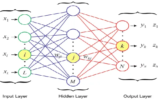
The Multilayer Perceptron network creates a non-linear mapping between input and output vectors by applying a multi-layer neural network. Figure (1) illustrates a multi-layer Multilayer Perceptron network.

Figure 1:.Schematic view of the MLP network

where 𝑥𝑖 , 𝑖 = 1,2, … , 𝑛 is the input data, 𝑤𝑖𝑗𝑘 ,

𝑗 = 1,2, … , 𝑚 represents the network weight which is

In this network, different layers are connected by means of their weights. When the network is in the training phase, the weights are set based on the difference between the desired output and the network output and by using different sushisen algorithms. One of the conventional methods to set the weights of network is the Steepest descend. This method is generally time-consuming due to the complexity of network and incapable of settingthe weight to minimize the network error [15]. To solve this problem, evolution methods can be effective. One of the mostly used evolution methods is PMO.The PMO method has been extensively used in many researches. Read on references (17, 18, 19, 20) for further study. The combination of PMO method and Multilayer Perceptron network and the adaptation of network weights to the PMO optimization process are discussed in the following section.

3.1. Adaption to network training

In this work, a three-layer Multilayer Perceptron network is used. W1 and W2 represent the weight

matrix between the input and hidden layer and between the hidden and output layer, respectively. Therefore, the weights are shown as particles in the PMO algorithm, and written as

𝑊𝑖 _{= 𝑊}

1𝑖, 𝑊2𝑖 (6)

Consequently, the position of each particle is given by

𝑃𝑖 _{= 𝑃}

1𝑖, 𝑃2𝑖 (6)

and Pb i

is the best member of the population and the velocity of particle i is denoted by Vj

i

.

Thus, the velocity formula in PMO method can be calculated by the following equation:

𝑉_{𝑗 ,𝑛𝑒𝑤}𝑖 = 𝑉_{𝑗 ,𝑜𝑙𝑑}𝑖 + 𝑣𝛼 𝑃_𝑗𝑖− 𝑊_𝑗𝑖 + 𝑠𝛽 𝑃𝑗𝑏𝑖

− 𝑊𝑗𝑖 /𝑡

𝑊𝑗 ,𝑛𝑒𝑤𝑖 = 𝑊𝑗 ,𝑜𝑙𝑑𝑖 + 𝑉𝑗𝑖

(7)

where s, v, and j=1,2 are positive constants, α and β are

random numbers between 0 and 1, and t is the time step and often equals to 1. The fitness function for the particle j in the form of output mean squared error is defined as

𝑓 𝑊𝑗 = 1 𝑠 𝑡𝑘𝑙

𝑜

𝑙=1 𝑠

𝑘=1

− 𝑃𝑘𝑙𝑊𝑗2

(8)

where f characterizes the fitness function, tkl is the

target output, PkL is the estimated output by the

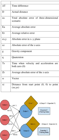
aforementioned network and based on weights W, s is the number of training samples and o is the number of neurons in the output layer. Figure (2) represents a schematic view of the fire detection intelligent network.

ΔT Time difference

D Actual distance

ea Total absolute error of three-dimensional scenario

Ea Average absolute error

Er Average relative error

ex,y Absolute error in x–y plane

ez Absolute error of the z-axis

g Gravity component

q Quaternion

Ts Time when velocity and acceleration are both zero (0)

Zr Average absolute error of the z-axis

ω Vector

xi Distance from start point (0, 0) to point (xe,ye)

0 200 400 600 800 1000 0

0.2 0.4 0.6 0.8 1

Time(s)

0 200 400 600 800 1000

0 0.2 0.4 0.6 0.8 1

Time(s)

Temprature CO Smog Flame

IV.

SIMULATION

The output data of sensor network is collected and denoted as Xmxn in which m indicates the number of

collected samples and n is the output BUS of the sensor network. In this simulation, the number of m=14980 and n=4 samples are collected using the sampling frequency of 0.1 Hz inside the room with various environmental conditions. Then the data set is

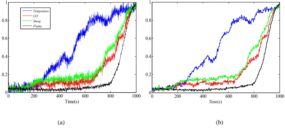
normalized. In the pre-processing section, the Mexican hat wavelet with the scale of V=3 is utilized. Meanwhile, the pre-defined threshold for the removal of non-essential principals is considered to be𝜎𝑡ℎ𝑟𝑒𝑠 ℎ𝑜𝑙𝑑 = %3. This means the data contains %97 of information of the primary data after pre-processing step. Figure (3) shows the resulted signals before and after pre-processing.

(a) (b)

Figure 3: A window plot of normalized sensor network data for (a). Noisy data and (b). Denoised data

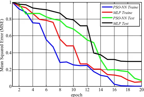
In the next step, the data enters PMO-NN network for training. The parameters used for the network training are given in Table 1. The results of network training are

shown in Figure (4).

Table 1: Proposed system parameters

Parameter Name Value Population Number 200

50 20 1e-5

rand(-10 10) Max. Iteration

Epoch Number Max. Error

Population initial value

As these figures indicate, the training and testing results are also drawn by steepest descentin order to compare the proposed method and the conventional Multilayer Perceptron. The results show that the new method is well able to predict the likelihood of fire with less error than the Multilayer Perceptron.

NO. OF PACKET DELIVERY

THROUGHPUT NODES RATIO

AODV DSDV AODV DSDV

10 1 0.904966 0.006668 0.006034

30

0.980403 0.79651 0.006536 0.005311

40 1 0.826577 0.006668 0.005512

50 1 0.914631 0.006667 0.006099

60

1 0.840805 0.006668 0.005607

70 0.999732 0.913557 0.006665 0.006092 80 0.980403 0.914094 0.006536 0.006095

90 1 0.914899 0.006668 0.006101

100

Figure 4: Performance comparison of the proposed method PSO-NN and MLP network for train and test

In order to measure the effects of pre-processing on the output of the proposed network, another simulation is conducted in which the PMO-Multilayer Perceptron input data is employed in both noised and denoised conditions. Figure (5) illustrates the output of the two different conditions. Here also, the RMS error resulted from applying pre-processed data in both training and testing modes is lower than that in the condition without pre-processing.

Figure 5: Performance comparison for training and testing PSO-NN for pre-processed and noisy data

It can be concluded that the noise in the data results in poor-training of network and consequently inaccurate output in testing.

SYSTEM DESCRIPTION: The experimental study has been conducted on a ASUS–X550C laptop with an Intel Core i3-3217U, 1.8 GHz CPU and with the RAM of 4GB, running in Windows 10.All programs are coded in MATLAB

Comparison on study

V.

CONCLUSION

In-time detection of fire is one of the challenges of modern life. On the other hand, the fire detection systems are always sought to be at the highest efficiency and yet with the lowest price. Therefore, using an intelligent detection method seems inevitable. In this paper, an intelligent method based on neural network is employed for the effective detection of fire. In order to overcome the problems of conventional neural networks, a method is proposed which uses PMO optimization method for training the neural network. Applying this method results in lower error in neural network. Furthermore, the Multilayer Perception-PMO neural network is utilized which enables the omission of error by combining wavelet decomposition and Generalized Singular Value Decomposition technique. It is concluded that the proposed network results in increasing data SNR and network precision.

REFERENCES

[1] A.T., Chan W.L. (1999) Fire Protection Systems. In: Intelligent Building Systems. The International Series on Asian Studies in Computer and Information Science, vol 5. Springer, Boston, MA,https://doi.org/10.1007/978-1-4615-5019-8_5.

[2] Aseeva R., Serkov B., Sivenkov A. (2014) Generation of Smoke and Toxic Products at Fire of Timber. In: Fire Behavior and Fire Protection in Timber Buildings. Springer

Series in Wood Science. Springer,

Dordrecht,https://doi.org/10.1007/978-94-007-7460-5_7. [3] A.T.P. & Chan, W.L. Fire Technol (1994) 30: 341. https://doi.org/10.1007/BF01038069.

[4] Wang Y., Ren X. (2012) An Intelligent Fire Alarm System Based on GSM Network. In: Zhao M., Sha J. (eds) Communications and Information Processing.

2 4 6 8 10 12 14 16 18 20

0 0.2 0.4 0.6 0.8 1

epoch

M

ea

n

S

qu

ar

ed

E

rr

or

(

M

S

E

)

PSO-NN Traine MLP Traine PSO-NN Test MLP Test

2 4 6 8 10 12 14 16 18 20

0 0.2 0.4 0.6 0.8 1

epoch

M

ea

n

S

qu

ar

ed

E

rr

or

(

M

S

E

)

Communications in Computer and Information Science, vol

289. Springer, Berlin,

Heidelberg,https://doi.org/10.1007/978-3-642-31968-6_28 [5] Wu, N., Yang, R. & Zhang, H. Build. Simul. (2015) 8: 579. https://doi.org/10.1007/s12273-015-0229-4

[6] Søreide, K., Thorsen, K. & Søreide, J.A. Eur J Trauma Emerg Surg (2015) 41: 91. https://doi.org/10.1007/s00068-014-0417-4

[7] Sheikh A.A., Lbath A., Warriach E.U., Felemban E. (2015) A Predictive Data Reliability Method for Wireless Sensor Network Applications. In: Wang G., Zomaya A., Martinez G., Li K. (eds) Algorithms and Architectures for Parallel Processing. Lecture Notes in Computer Science, vol 9532. Springer, Cham,https://doi.org/10.1007/978-3-319-27161-3_59

[8] Yuan DP., Li Z., Li M. (2017) Research on Indoor Firefighter Positioning Based on Inertial Navigation. In: Harada K., Matsuyama K., Himoto K., Nakamura Y., Wakatsuki K. (eds) Fire Science and Technology 2015. Springer, Singapore,https://doi.org/10.1007/978-981-10-0376-9_48

[9] Kågström, B. BIT (1984) 24: 568. https://doi.org/10.1007/BF01934915

AUTHORS PROFILE