A Mathematical Model for Monitoring Laboratory
Revenue Accrued from Tests
Jessica Chinezie Benson-Iyare
Department of Computer Science Federal Polytechnic, Idah, Nigeria
H. A. Soriyan
Department of Computer Science and Engineering Obafemi Awolowo University, Ile-Ife, Nigeria
ABSTRACT
One challenge in the laboratory is the discrepancies in the revenue reported to have been generated and the actual revenue generated from laboratory tests. In this paper, a mathematical model for tracking and monitoring revenue from hospital-based laboratory was formulated, simulated, and evaluated.
The mathematical model was formulated using a multiple variable linear equation. The model was simulated using Matrix Laboratory (MATLAB) and evaluated for accuracy using the following performance metrics: Correlation coefficient, Mean absolute error, Root mean square error, Relative absolute error and Root relative squared error. Multivariate linear regression analysis method was used for the evaluation in Waikato Environment for Knowledge Analysis software (WEKA). Dataset for the simulation were retrieved from a government hospital-based laboratory in Idah, Nigeria. The result of the study showed that a multiple variable linear equation is sufficiently adequate in relating the revenue generated with the tests performed in hospital laboratory. Furthermore, the study revealed discrepancies in the revenue reported to have been generated from the laboratory tests. The regression analysis showed that the distribution of data for the classes of datasets have strong statistical relationship between tests and the revenue generated with a correlation coefficient of 0.9985 and 0.8113 respectively.
In conclusion, the study established that the formulated multi-variate linear relationship between revenue and tests is appropriate in predicting revenue generated from hospital-based laboratory.
General Terms
LaboratoryKeywords
Laboratory, Hospital, Model, Revenue, Monitoring, Regression, multiple variable linear equation, simulation, mathematical model, evaluation, multivariate linear regression analysis
1.
INTRODUCTION
The Clinical or Medical laboratory forms part of the total economic structure of the hospital. It generates revenue for the hospital to undertake various activities to uplift it [1]. The hospital’s laboratory is constituted not only for service-seeking motive but apparently as an instrument of generating revenue and as such must work towards achieving the hospital’s set objectives [2], [9]. The clinical laboratory makes the bulk of its revenue by performing physician ordered tests otherwise known as investigations which the hospital management always seeks to maximize [3], [4]. A typical laboratory's
revenue stream is predictable when the laboratory manager knows the existing customer base and the rough number, or average volume of test orders usually placed for a given period of time. As the laboratory market continues to become more complex, laboratories make great efforts to be efficient and collect money expediently for the services they provide. The role of hospital based laboratory in the overall development of the hospital cannot be over emphasised. As a revenue generating department, it is expected to be able to give accurate account of how many tests the laboratory runs and how much is accrued from them. One challenge though is that there are discrepancies in the revenue reported to have been generated and the actual revenue generated from the laboratory tests. This study designs a mathematical model that will track the number of laboratory tests in order to accurately determine how much revenue is generated from them and monitor revenue generated from these laboratory tests.
2.
LITERATURE REVIEW
A clinical laboratory is where tests are done on clinical specimens in order to get information about the health of a patient as pertaining to the diagnosis, treatment, and prevention of disease [5]. Specimens are collected, tests are performed, and results are reported in the clinical laboratory. A typical workflow includes doctor ordering the test, collecting and labelling patient sample, delivering samples to the laboratory, processing sample, analysing test (sample), and reporting results to doctor.
group of physicians and perform routine laboratory tests on their patients.
Laboratories provide important information support for the diagnosis, prevention, or treatment of any disease to assess the health of human beings and improve the wellbeing of patients [11]. The results of laboratory investigations provide invaluable tools for making decisions. They also facilitate the initiation and monitoring of appropriate clinical and public health interventions [10]. As revenue centres within the hospitals, saddled with the responsibility of bringing significant revenue streams, laboratories sometimes face data constrictions that prevent them from accurately measuring fiscal performance [9].
In most cases, laboratories experience a revenue leakage whereby laboratory investigations are done but not charged yielding into non-collection of payments for the services not charged or the full money is not collected. It is a universal phenomenon gnawing up the profit margin of services in the hospital-based laboratory. It can occur as a result of incorrect pricing, missing transactions, and uncollected revenue. Revenue leakage is common, but often unnoticed because it is not easily found in financial statements [6]. Revenue is the money that an organisation receives from its business. In essence, revenue accrued from the laboratory is the money that the hospital receives from the services rendered in the laboratory; in this case, the laboratory tests.
3.
METHODS AND MATERIALS
3.1
Research Approach
This research used the empirical approach predicated on the need to get precise comprehensive and reliable information. Empirical approach is based on observed and measured phenomena, that is, acquiring data by means of observation or experimentation for statistical analysis [7].
3.2
Area of Study
The research was conducted in a government hospital in Idah, Kogi State, Nigeria. Kogi State is in the North Central geopolitical zone of the six states structure organised into six political configurations.
3.3
Data Collection Method
Two months laboratory record books were collected from the hospital, in the Period February 2014 to March 2014 in order to observe the processes involved in a patient consulting a doctor, paying for laboratory tests, and getting a patient to perform laboratory tests. Secondary data were also collected from laboratory documents, laboratory journals, and the Internet.
3.4
Mathematical Model Formulation for
Tracking and Monitoring Laboratory
Revenue
The mathematical model to track and monitor revenue generated from the hospital’s laboratory was formulated in this section based on the dataset collected from the hospital’s laboratory under study. This is in view of simulating a process that can monitor the revenue generated from the tests conducted in the laboratory. Simulation is the process of using a model to study the behaviour and performance of an actual or theoretical system [8]. This is in order to predict the actual behaviour of the system.
3.4.1
Variable Description of the Datasets
There are three different classes of variables from the dataset got from the hospital used as case study. These variables were used in monitoring the revenue generated by the laboratory. The variables are as follows:
a. The daily number of tests performed in the laboratory;
b. The respective prices of each test; and c. The revenue generated for each test performed. Test price and the number of test performed are the Independent Variables while the revenue generated for each test performed is the Dependent Variable. The amount made from the laboratory depends on the number of tests performed and their respective prices.
3.4.2
The tests performed in the laboratory
There are a total of 30 tests which are performed out of which twenty-five (25) tests are paid for while five (5) tests are free. Three (3) out of the five (5) tests performed for free are totally free for all patients and the remaining two (2) free tests are free for only HIV patients. The remaining two (2) tests are free for only HIV patients. There are also two (2) different classes of patients for whom tests are performed – National Health Insurance Scheme (NHIS) patients and Non-National Health Insurance Scheme (Non-NHIS) patients (regular patients) and two (2) different classes of tests – paid tests and free tests. Hence, there are four (4) different classes of datasets which are monitored by the model. They are:
a. The tests performed for regular (Non-NHIS) patients; b. The tests performed for NHIS patients;
c. The free tests performed for regular (Non-NHIS) patients; and
d. The free tests performed for NHIS patients.
The revenue of the dataset of the laboratory which is chosen will be monitored by the model in order to validate the value of revenue expected given the number of tests performed in a particular period of time and the prices of each test performed. The datasets for this research are tests performed within the period of February 2014 till March, 2014. Table 3.1 shows the breakdown of the different tests and their respective prices.
3.4.3
The Revenue Generated from the different
Tests Performed in the Laboratory
The revenue generated by the laboratory staff is expressed as a sum of the daily cost of each test performed in Naira (N). It is a polynomial equation of One (1) degree and multiple variables, Xi (the price of each test), and ai (the number of unit test). The
equation is otherwise referred to as a multiple variable linear equation with the output R as the total revenue while the intercept a0 = 0 was used to define the total revenue generated for any test performed for each day (See equation 3.1a). Putting the variables together; Revenue generated for any test performed for each day is expressed as given in equation 3.1a.
Where
is the number of tests performed for every test, i (where 0 < i <= n) and n is the total number of tests performed and Xi is the price for each test, i.
Hence, n = 25 for regular tests, n=5 for free tests and Xi is the
cost of each test, i. For any given time period, j (where 0 < j <= m), where m is the number of days for which tests were performed and Rj is the total revenue generated within a period
of j days. (See Equation 3.2a).
Or simply as
Where
is the number of tests performed for every
test, i (where 0 < i <= n); n is the total number of tests for every single day, j (where 0 < j <= m) and Xi is the cost of each
test, i.
3.5
The Mathematical Model for Monitoring
Laboratory Revenue
The mathematical model which was used in monitoring the revenue generated for every test performed in the laboratory requires certain variables. The variables needed by the monitoring model are:
a. The total number of tests performed for every day; b. The price for each test performed; and
c. The total revenue generated for the tests.
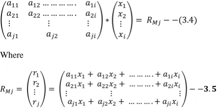
Equations 3.2a and 3.2b can equally be expressed in matrix form in as represented in equation 3.3 from which the monitored revenue may be determined:
Such that:
Aji = the amount (number) of tests, i that were performed
within a specified period of time, j days.
Xi = the test price for each test, i and
RM = the revenue monitored by the model over a period of j days.
The monitoring model collects all the daily total tests performed and expresses them as a square matrix (of dimension-n, where n > 25 for regular tests and n>5 for free tests). Hence, the daily number of tests performed in the laboratory is expressed as a matrix of dimension-n; the price of each test is also expressed as a column matrix of dimension-n. The monitored revenue, RMj is the result of the product of both
matrix which results in a column matrix of similar dimension - n = j. (See equation 3.4).
Where
After determining the monitored revenue, RMj by the model;
this value was compared with the actual revenue, RA collected
from the laboratory for all four (4) classes of data. The difference between the monitored and actual revenue is determined in order to find out any likely difference. If there is any difference recorded, the date that corresponds with the record is checked for errors. So, the difference is defined by a column matrix of dimension-n stated as follows:
Hence, if
Thus, equation 3.3 is the mathematical model for monitoring laboratory revenue.
Table 3.1 Breakdown of the different tests and their respective prices
I Test (Xi) Amount (N)
1. Packaged Cell Volume (PCV) 200
2. +Malaria Parasite (MP) 200
3. Widal 250
5. Genotype 500
6. Pregnancy Test (PT) 250
7. Pregnancy Test (PT)-Serum 300
8. 9. Hepatitis B Virus Hepatitis C Virus 300
300
10. Syphilis 300
11. Culture tests 700
12. Urinalysis (Urine) 200
13. Urine M/C/S 500
14. Sputum M/C/S 500
15. Semen M/C/S 700
16. Semen Analysis 500
17. Stool Analysis 200
18. High Vaginal Swab (HVS) 500
19. Ante Natal Care (ANC) services 1000
20. ESR (Erythrocyte Segmentation Rate) 500
21. Full Blood Count (FBC) 500
22. Fasting Blood Sugar (FBS) 300
23. Random Blood Sugar (RBS) 300
24. Liver Function Test (LFT) 2000
25. Kidney Function Test (KFT) 2000
26. Electrolyte, Urea & Cretinin 3000
27. +Prostrate Surface Antigen (PSA) 1500
28. *Acid-Fast Bacilli (AFB) Sputum (Tuberculosis test) 2500
29. * Human Immunodeficiency Virus screening (HIV test) 700
30. *Cluster of Differentiation 4 CD4 (HIV test) 1000
3.6
Model Assumptions
The following assumptions were made in the formulation of the mathematical model.
a. Consumables, Reagents and Drugs are available. b. Equipment, Apparatus, Water Supply and Power
Supply are set.
c. All tests taken are paid for except for the eligible patients for free tests.
d. All tests paid for are performed.
3.7
Software Used for Simulation and
Evaluation
The software used for simulating and evaluating the mathematical are:
a. Matrix Laboratory software (MATLAB)
The MATLAB software is basically a collection of different toolboxes which can be used to perform a variety of different functions and the version used is the MATLAB R2009a version 7.8.0. The variables in MATLAB are stored as arrays and matrices. This is suitable for monitoring the revenue generated in the laboratory for the respective classes of tests. The MATLAB software was used in simulating the monitoring of the revenue generated for each class of tests performed using the value of the difference calculated and
b. Waikato Environment for Knowledge Analysis software (WEKA). The WEKA software is java-based software which performs various types of data mining tasks such as; classification, clustering, association etc. The version of software used is WEKA 3.7.1 and the software’s regression modelling algorithm (classifiers) is suitable for evaluating the performance of the monitoring model by performing the least squares algorithm in order to generate the linear regression equation used in plotting the revenue generated and in determining the correlation and error rates. WEKA uses least square method in developing the linear regression model.
4.
RESULTS AND DISCUSSION
This section discusses the findings from the hospitals under survey. It describes the datasets used in monitoring the revenue generated from the laboratory. It also presents the results of the simulation and the performance evaluation of the mathematical model.
4.1
Classification of Laboratory Data
The data collected at the laboratory were classified into four (4) different categories which are described as follows:
a. Daily tests and revenue generated for regular patients;
b. Daily tests and revenue generated for NHIS patients; c. Daily free tests and revenue generated for regular
patients; and
d. Daily free tests and revenue generated for NHIS patients.
4.2
Revenue generated for the daily tests
performed on regular (Non-NHIS)
patients
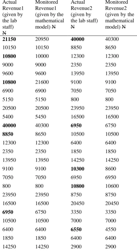
As stated earlier, the mathematical model was simulated using MATLAB software. The monitoring model collects and stores the data collected for the total tests performed in a 25 by 25 matrix – so the dataset for regular patients was stored in two different Matlab files. The test price for each test was also stored in a column matrix (25 by 1):
a. dailyTests1.mat: which contains tests performed for the first 25 days;
b. dailyTests2.mat: which contains tests performed in the last 25 days; and the test price stored as
c. TestsPrice.mat
Following is a section of the Matlab code used in executing the process:
To generate the revenue for the first 25 days >>> dailyTests1=load (‘dailyTests1.mat’) >>>TestsPrice=load (‘TestsPrice.mat’) >>>Revenue1=dailyTests1*TestsPrice To generate the revenue for the first 25 days
>>> dailyTests2=load (‘dailyTests2.mat’) >>>TestsPrice=load (‘TestsPrice.mat’) >>>Revenue2=dailyTests2*TestsPrice
The results of the Matlab implementation of the value of the revenue generated for each dataset is shown in Table 4.1.
Table 4.1 Results of the Monitoring Model for Regular (Non-NHIS) Patients’ Tests
Actual Revenue1 (given by the lab staff) N Monitored Revenue1 (given by the mathematical model) N
Actual Revenue2 (given by the lab staff) N
Monitored Revenue2 (given by the mathematical model) N
21150 20950 40000 40300
10150 10150 8850 8650
10800 10000 12300 12300
9000 9000 2350 2350
9600 9600 13950 13950
10800 21600 9100 9100
6900 6900 7050 7050
5150 5150 800 800
20500 20500 23950 23950
5400 5450 16500 16500
40000 40300 6950 6750
8850 8650 10500 10500
12300 12300 6400 6400
2350 2350 1850 1850
13950 13950 14250 14250
9100 9100 10300 8600
7050 7050 6950 6950
800 800 10800 10600
23950 23950 8750 8750
16500 16500 20450 20450
6950 6750 3350 3350
10500 10500 7000 7000
6400 6400 6550 4550
1850 1850 6400 6400
14250 14250 2900 2900
It can be concluded from the results presented in table 4.1 that if the calculated value is equal to the actual value of the
revenue; one can say that the revenue collected is not questionable and free from errors and if the calculated value is different from the actual value of the revenue; then the revenue collected is questionable.
The results of the monitoring model above shows that there are six (6) errors out of the total 25 data provided by the laboratory staff which can be queried for difference in values – in some cases the value is less while in some the value is greater. For the second data set which contains tests performed for the last 25 days – five (5) errors were observed. It therefore means that the monitoring model was able to detect errors in the revenue provided by the laboratory staff.
4.3
Revenue generated for the daily tests
performed on NHIS patients
The monitoring model collects and stores the data collected for the total tests performed in a 25 by 25 matrix – so the dataset for NHIS patients was stored into two different Matlab files. The test price for each test was also stored in a column matrix (25 by 1):
a. NHISTests1.mat: which contains tests performed for the first 25 days;
b. NHISTests2.mat: which contains tests performed in the last 25 days; and the test price stored as
c. TestsPrice.mat
Following is a section of the Matlab code used in executing the process:
To generate the revenue for the first 25 days >>> NHISTests1=load (‘NHISTests1.mat’) >>>NHISPrice=load (‘TestsPrice.mat’) >>>NHISRevenue1=NHISTests1*TestsPrice To generate the revenue for the first 25 days
>>> NHISTests2=load (‘NHISTests2.mat’) >>>NHISPrice=load (‘TestsPrice.mat’) >>>NHISRevenue2=dailyTests2*TestsPrice The results of the Matlab implementation of the value of the revenue generated for the dataset is shown in Table 4.2.
Table 4.2 Results of the Monitoring Model for NHIS Patients’ Tests Actual Revenue1 (given by the lab staff) N Monitored Revenue1 (given by the mathematical model) N
Actual Revenue2 (given by the lab staff) N Monitored Revenue2 (given by the mathematical model) N
3200 3200 2100 2100
750 750 3350 2550
2500 2500 1400 1400
1150 1150 5500 5500
1800 1800 300 300
1800 1800 1100 1100
1000 1000 1500 1500
2100 2100 600 600
2550 2550 1100 1100
1400 1400 700 700
5500 5500 650 650
300 300 300 300
1500 1500 1850 1850
600 600 1650 1650
1100 1100 3700 3700
700 700 1350 1350
650 650 1100 1100
300 300 1200 1200
300 300 3000 3000
1850 1850 2350 2350
1650 1650 1450 1450
3700 3700 700 700
1350 1350 1200 1200
1100 1100 2550 2550
Again, it can be concluded from the results presented in table 4.2 that if the calculated value is equal to the actual value of the revenue; one can say that the revenue collected is not questionable and free of errors and if the calculated value is different from the actual value of the revenue; then the revenue collected is questionable.
The results of the monitoring system show that there are no errors out of the total 25 data provided by the laboratory. For the second data set which contains tests performed for the last 25 days – only one (1) error was observed from the results plotted by the monitoring system; hence, the data may be queried for the respective error. This also follows again that the monitoring system was able to detect errors in the revenue provided by the laboratory staff.
4.4
Model Evaluation
The revenue generated is expressed as a linear equation of one degree. The monitoring model was evaluated using the multi-variate linear regression analysis method. The value of the monitored revenue generated was compared with the actual revenue generated with the aim of measuring the error rate (which determines the accuracy) of the generated regression model.
The standard linear regression model has the form:
4.1
Where the
j’s are unknown parameters or coefficients and the idea is to have a set of data of the form; (x1, y1), (x2,y2),..,(xp, yp) from which the value of
jfor j=1…p can bedetermined.
Least squares method is the most widely used procedure for developing estimates of the model parameters. Thus it was used to estimate the values of the parameters (coefficients) of the model based on the observed n sets of values. βs are values to be estimated.
There are two important things to note when using least squares method for modeling:
i. Prediction Accuracy: least squares estimates often provide predictions with low bias but high variance; and ii. Interpretation: when the number of regressors, I is too
high, the model is difficult to interpret. One seeks to find a smaller set of regressors with higher effects.
The model used in monitoring the revenue generated from the tests performed in the laboratory for regular patients and NHIS patients was evaluated using WEKA software. The dataset used for the analysis was partitioned as:
a. The dataset containing the revenue for tests performed for regular patients; and
b. The dataset containing the revenue for tests performed for NHIS patients.
The results of the evaluation of the model using WEKA is shown in Table 4.3 and 4.4. The error values, correlation coefficient, mean absolute error, mean square error, relative absolute error and the root absolute square error were also determined (see Table 4.5).
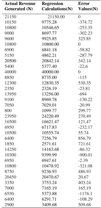
Table 4.3 Results of Regression Analysis of the Dataset for the Tests Performed on Regular Patients
Actual Revenue Generated (N)
Regression Calculations(N)
Error Values(N)
21150 21150.00 0
10150 9775.28 -374.72
10800 10546.65 -253.35
9000 8697.77 -302.23
9600 9925.85 325.85
10800 10800.00 0
6900 6841.18 -58.82
5150 4862.21 -287.79
20500 20842.14 342.14
5400 5377.40 -22.6
40000 40000.00 0
8850 8735.00 -115
12300 12830.35 530.35
2350 2326.19 -23.81
13950 13256.00 -694
9100 8969.78 -130.22
7050 7029.01 -20.99
800 1099.77 299.77
23950 24220.49 270.49
16500 16621.47 121.47
6950 6717.83 -232.17
10500 10555.74 55.74
6400 7256.79 856.79
1850 2571.61 721.61
14250 14163.68 -86.32
10300 9399.99 -900.01
6950 6947.61 -2.39
10800 10478.92 -321.08
8750 9236.93 486.93
20450 20470.67 20.67
3350 3753.24 403.24
7000 7165.19 165.19
6550 5373.88 -1176.1
6400 6291.71 -108.29
2900 3409.68 509.68
pj j j
x
X
f
1 0
)
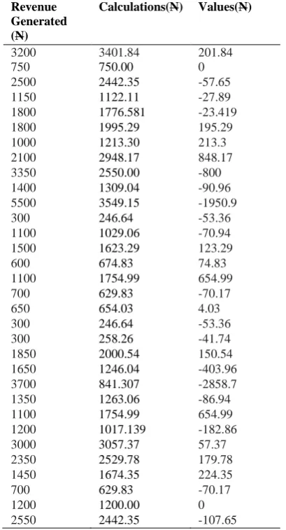
Table 4.4Results of Regression Analysis of the Dataset for the Tests Performed on NHIS Patients. Actual
Revenue Generated (N)
Regression Calculations(N)
Error Values(N)
3200 3401.84 201.84
750 750.00 0
2500 2442.35 -57.65
1150 1122.11 -27.89
1800 1776.581 -23.419
1800 1995.29 195.29
1000 1213.30 213.3
2100 2948.17 848.17
3350 2550.00 -800
1400 1309.04 -90.96
5500 3549.15 -1950.9
300 246.64 -53.36
1100 1029.06 -70.94
1500 1623.29 123.29
600 674.83 74.83
1100 1754.99 654.99
700 629.83 -70.17
650 654.03 4.03
300 246.64 -53.36
300 258.26 -41.74
1850 2000.54 150.54
1650 1246.04 -403.96
3700 841.307 -2858.7
1350 1263.06 -86.94
1100 1754.99 654.99
1200 1017.139 -182.86
3000 3057.37 57.37
2350 2529.78 179.78
1450 1674.35 224.35
700 629.83 -70.17
1200 1200.00 0
2550 2442.35 -107.65
4.5
The Performance or Evaluation Metrics
The performance or evaluation metrics used by the WEKA software to evaluate the regression model are: Correlation coefficient, mean absolute error, root mean square error, relative absolute error and root relative squared error.
4.5.1
Correlation coefficient
The correlation coefficient (r) measures the strength and the direction of a linear relationship between two variables. The linear correlation coefficient is sometimes referred to as the Pearson Product moment correlation coefficient in honour of its developer Karl Pearson.
4.5.2
Mean absolute error (MAE)
Mean absolute error is used to forecast accuracy by comparing the forecast value to the actual value. The mean absolute error is the mean of the absolute errors. The absolute error is the absolute value of the difference between the forecast value and the actual value. MAE tells us how big of an error we can expect from the forecast on average. MAE calculates the mean absolute error function for the forecast and the eventual outcomes.
4.5.3
Root mean square error (RMSE)
Root mean square error is calculated to adjust for large rare errors. This is done by squaring the errors before we calculate their mean; we arrive at a measure of the size of the error that gives more weight to the large but infrequent errors than the mean. RMSE is used to measure the differences between values predicted by a model and the value actually observed. The RMSE serves to aggregate the magnitudes of the errors in predictions for various times into a single measure of predictive power. It is a good measure of accuracy, but only to compare forecasting errors of different models for a particular variable and not between variables, as it is scale dependent.
4.5.4
4.5.4
Relative absolute error (RAE)
Relative absolute error is relative to a simple predictor which is just the average of the actual values. The error is the total absolute error. Thus, the relative absolute error takes the total absolute error and normalises it by dividing by the total absolute error of the simple predictor.
4.5.5
4.5.5 Root relative squared error (RRSE)
Root relative squared error is computed by dividing RMSE by the RMSE obtained by just predicting the mean of target values (and then multiplying by 100). Therefore, smaller values are better and values greater than 100% indicate a scheme is doing worse than just predicting the mean. RAE is computed in a similar manner.
Table 4.5 Results of the evaluation metrics Performance metrics Regular
Tests data
NHIS Tests data Correlation Coefficient 0.9985 0.8113 Mean absolute error 291.9947 318.0787 Root mean square error 410.3096 670.2791 Relative absolute error 5.717% 35.6456% Root relative squared error 5.4965% 57.5625%
Figure 4.1 Line chart representation of the results of the evaluation metrics
0 100 200 300 400 500 600 700 800
Regular Tests data
From the results of the regression analysis, the distribution of data for both classes of datasets (regular and NHIS patients) showed strong positive relationships between the tests and the revenue generated with a correlation coefficient of 0.9985 and 0.8113 respectively. In statistics, a correlation expresses the strength of relationship between two variables in a single value between -1 and +1. High correlation coefficient increases the accuracy of prediction. The regression model is statistically significant if the level of significance (ρ-value) < 0.01 and the regression model is statistically insignificant if the level of significance (ρ-value) > 0.01. Thus, the regression analysis for regular patients shows a high level of significance of 0.0015. MAE measures how far predicted values are away from observed values. Lower values of RMSE indicate better fit. The larger the error the less relationship between the tests and the revenue generated. The RMSE was calculated to adjust the large rare errors.
5.
CONCLUSION
The focus of this research is to design a mathematical model for monitoring revenue in a hospital-based laboratory. This was done by tracking the number of tests and their corresponding amounts. To actualize the aim and objectives in this research, a mathematical model was formulated to track and monitor laboratory revenue. Findings from the hospital under study showed that there are discrepancies in the revenue reported to have been generated and the actual revenue generated from the laboratory tests as shown in the simulation results. This is as a result of improper documentation of the laboratory tests performed and the revenue generated from them. Due to this, revenue is misstated because of loss of track of laboratory tests counts. Some laboratory staff collect money from the patients to pay on their behalf. These staff do not make the payments and as such they do not have evidences of payment. This is revenue leakage. This study had used only two (2) months records, further study should utilise records for more years to get large data set in order to determine the trend of the revenue and for a more detailed analysis.
6.
REFERENCES
[1] Mangels, J. I. (2008). Cost Effective Clinical Microbiology. California Association for Medical Laboratory Technology. DL-984. 1-25.
[2] Eze, J. C. (2013). Evaluation of Fraud and Internal Control Procedures: Evidence from Two South East Government Ministries in Nigeria. Research Journal of Finance and Accounting. 4(17): 63-70.
[3] Neumann, D. and Pueschel, T. (2009). Management of Cloud infrastructures: Policy-based Revenue of Optimization. Association of Information Systems Electronic Library (ICIS). Proceedings. 178.
[4] Vikica, B., Hrvoje, P., and Mladen, P. (2011). Clinical laboratory as an economic model for business
performance analysis. Clinical Sciences doi: 10.3325/cmj.52.513.
[5] Michael, F. J. and Shatkin, L. (2004). Best jobs for the 21st century. JIST Works. 460. ISBN 1-56370-961-9. [6] Wyman, O. (2006). Reducing Revenue Leakage.
www.oliverwyman.com. Retrieved on March 25, 2014. [7] Ramesh, V., Glass, R., and Vessey, I. (2004). Research in
computer science: an empirical study. The Journal of Systems and Software, 70: 165-176.
[8] Di Caro, G. A. (2003). Analysis of simulation environments for mobile ad hoc networks. Technical Report No. IDSIA-24-03, Dalle Molle Institute for Artifcial Intelligence, Galleria 2, 6928 Manno, Switzerland.
[9] Fetter, K. (2017). Revenue Cycle Management Challenges
in Laboratory Outreach.
http://www.beckershospitalreview.com/finance/ revenue-cycle-management-challenges-in-laboratory-
outreach.html. Retrieved on 11/05/2018.
[10] Adane, K., Abiyi, Z., and Desta, K. (2015). The Revenue Generated from Clinical Chemistry and Hematology Laboratory Services as Determined using Activity-Based Costing (ABC) Model. Cost Effectiveness and Resource Allocation 13(20): 1-7.
[11] Manickam, T. S. and Ankanagari, S. (2015). Evaluation of Quality Management Systems Implementation in Medical Diagnostic Laboratories Benchmarked for Accreditation. Journal of Medical Laboratory and Diagnosis. 6(5): 27-35.
7.
AUTHOR’S PROFILE
Benson-Iyare, Jessica Chinezie holds a Master degree in Computer Science from Obafemi Awolowo University, Ile-Ife, Nigeria and a Bachelor of Science degree in Computer Science from the University of Ado-Ekiti, Nigeria. She is a member of Nigeria Computer Society and Nigerian Institute of Management (Chartered). Her interest includes Information Systems Development with emphasis on Education. She is currently researching Adaptive Learning Systems. She has published some journal and learned conference articles. She is a lecturer in the Department of Computer Science at the Federal Polytechnic Idah, Nigeria.
Professor Soriyan, H. A. is a professor in the Department of Computer Science and Engineering, Obafemi Awolowo University, Ile-Ife, Nigeria. She has over 25 years of experience in teaching and research. Her interests include information systems development with emphasis on healthcare. She has published a good number of journal and learned conference articles, and made useful contributions to books.
8.
APPENDIX I
Results of the regression analysis on the regular patients’ tests
=== Run information ===Scheme: weka.classifiers.functions.LinearRegression -S 0 -R 1.0E-8 Relation: dailyRevenue
MP Widal Blood group HP-Genotype PT
PT-serum HPV-B and C Syphillis CT Urine Urine M/C/S Sputum M/C/S semen M/C/S Semen Stool HVS ANC ESR FBC FBS RBS LFT KFT Electrolyte Total Revenue (N)
Test mode: evaluate on training data === Classifier model (full training set) === Linear Regression Model
Total Revenue (N) = 190.326 * PCV+ 251.5078 * MP + 176.7534 * Widal + 421.2725 * HP-Genotype + 284.8327 * PT +
-4340.1466 * HPV-B and C + 1755.2226 * semen M/C/S + 468.5118 * HVS + 988.4857 * ANC + 3313.1218 * FBC + 377.3805 * FBS + 1656.5604 * LFT + 3273.599 * Electrolyte + 719.1165
14 2350 2326.189 -23.811 15 13950 13256.002 -693.998 16 9100 8969.784 -130.216 17 7050 7029.007 -20.993 18 800 1099.768 299.768 19 23950 24220.49 270.49 20 16500 16621.468 121.468 21 6950 6717.834 -232.166 22 10500 10555.744 55.744 23 6400 7256.79 856.79 24 1850 2571.606 721.606 25 14250 14163.682 -86.318 26 10300 9399.991 -900.009 27 6950 6947.606 -2.394 28 10800 10478.917 -321.083 29 8750 9236.925 486.925 30 20450 20470.674 20.674 31 3350 3753.237 403.237 32 7000 7165.191 165.191 33 6550 5373.883 -1176.117 34 6400 6291.71 -108.29 35 2900 3409.675 509.675 === Evaluation on training set ===
Time taken to test model on training data: 0.04 seconds === Summary ===
Correlation coefficient 0.9985 Mean absolute error 291.9947 Root mean squared error 410.3096 Relative absolute error 5.717 % Root relative squared error 5.4965 % Total Number of Instances 35
9.
APPENDIX II
Results of the regression analysis on the NHIS patients’ tests
=== Run information ===Scheme: weka.classifiers.functions.LinearRegression -S 0 -R 1.0E-8 Relation: NHISRevenue
Instances: 32 Attributes: 26 PCV MP Widal Blood group HP-Genotype PT
Test mode: 10-fold cross-validation === Classifier model (full training set) === Linear Regression Model
Total Revenue (N) = 255.9122 * PCV + 128.1614 * MP + 348.5625 * Widal + 418.0404 * HP-Genotype + 432.0782 * PT +
244.831 * Urine + 1086.4857 * ANC + 408.71 * FBS + 322.1076 * RBS + 2045.0851 * LFT + 2861.8998 * Electrolyte + -154.2175
Time taken to build model: 0 seconds === Predictions on test data === inst# actual predicted error 1 700 1034.626 334.626 2 2550 2480.845 -69.155 3 1100 1754.994 654.994 4 1400 1309.038 -90.962 5 1450 1674.345 224.345 6 1800 1776.581 -23.419 7 700 629.833 -70.167 8 2500 2442.35 -57.65 9 300 258.255 -41.745 10 3700 841.307 -2858.693 11 600 674.828 74.828 12 3350 2550 -800 13 750 750 0 14 1200 1200 0 15 1100 1029.06 -70.94 16 1100 1029.06 -70.94 17 300 243.419 -56.581 18 1200 1017.139 -182.861 19 1800 1995.289 195.289 20 1650 1246.044 -403.956 21 300 246.64 -53.36 22 650 654.03 4.03 23 3000 3057.366 57.366 24 5500 3549.153 -1950.847 25 2350 2529.779 179.779 26 1850 2000.544 150.544 27 1500 1623.293 123.293 28 1000 1213.304 213.304 29 1150 1122.111 -27.889 30 2100 2948.166 848.166 31 3200 3401.844 201.844 32 1350 1263.057 -86.943 === Cross-validation ===
=== Summary ===