Profile Gear Grinding Temperature Reduction and Equalization

(1)

Journal of Engineering Sciences, Volume 5, Issue 1 (2018), pp. A 1–A 7 A 1 JOURNAL OF ENGINEERING SCIENCES

УРНА ІН Н РН Х НАУ

УРНА Н Н РНЫХ НАУ

Web site: http://jes.sumdu.edu.ua

DOI:

10.21272/jes.2018.5(1).a1

Volume 5, Issue 1 (2018)

UDC 621.923.1

Lishchenko N. V.1, Larshin V. P.2

1

Odessa National Academy of Food Technologies, 112 Kanatna St., Odessa, 65039, Ukraine;

2

Odessa National Polytechnic University, 1 Shevchenka Av., Odessa, 65044, Ukraine

Article info: Paper received:

The final version of the paper received: Paper accepted online:

December 29, 2017 February 3, 2018 March 5, 2018

*Corresponding Author’s Address:

[email protected]

Abstract. The profile gear grinding modes definition technique is developed to provide the uniform residual tem-peratures after heating and subsequent cooling which predetermine uniform thermal deformations on periphery of a cogwheel when grinding. The initial basis for this is a possibility to determine the gear grinding temperature both on the heating and cooling stages and, besides, it is may be also a choice of the operation cycle structure with and with-out the working stroke omission. In the interval of the profile gear grinding modes, two variants of the gear grinding working cycle structure with reciprocating displacement of the grinding wheel are considered using the simulation method with an omission and without one of the working stroke. Certain combinations of mode parameters are found in the range of their possible values at which the combination of heating and cooling leads to the lowest residual sur-face temperature both during and after working stroke.

Keywords: profile gear grinding, gear grinding temperature, heating stage, cooling stage, cycle structure, working stroke, temperature.

1 Introduction

Typically grinding modes are selected according to reference statistical tables [1]. The choice of them is not substantiated by any criterion, for example, a criterion of the absence of grinding burns, a criterion of the grinding wheel life, a criterion for uniform heating of the machin-ing cogwheel on its periphery, etc.

It is known the method of determining the modes of profile grinding in the three successive stages of this op-eration according to the system-wide principle of stage theory for any technical process. These stages are rough, semifinish, and finish ones and each of them depends on grinding temperature [2]. A peculiarity of the third grind-ing stage is the need to equalize the temperature heatgrind-ing along the periphery of a cogwheel. There is a rule that at the finishing stage, the infeed value should be such that it would be possible to grind all the cogwheel teeth without dressing the profile grinding wheel [3]. This is due to the fact that after the dressing, the grinding wheel changes its cutting capacity and the position line of the cutting edge. The infeed value at the finishing stage is reduced as the grinding stock for this stage decreases, and at the last grinding working stroke it is not recommended to apply the infeed values less than 0.010...0.015 mm [2].

Howev-er, these data are also not substantiated by any objective criterion and are more likely to be the result of practice.

In the paper [4] the three staged structure of the gear grinding operation is analyzed and consists of rough, semifinish and finish stages. Moreover, modes for each stage are selected based on the parameters of the specific material removal rate in mm3/(s·mm) and the specific material removal in mm3/mm. However, these are formal indicators which are not related, for example, to the grinding temperature and the grinding wheel wear.

The purpose of the paper is to improve the method of determining the grinding modes on the last finish (third) stage of the machining cycle by establishing a connection between formal indicators mentioned and the grinding temperature.

2 Research Methodology

2.1 Initial equations

(2)

A 2 MANUFACTURING ENGINEERING: Machines and Tools cogwheel heat content. The temperature field at the

heat-ing stage is described by a mathematical dependence, which is a solution of a one-dimensional differential equation of heat conductivity. To determine the tempera-tureTH( ,x H) at the heating stage, we can use the equa-tion [5]

0 2

( , ) ierfc

2

H H H

H

q x

T x a T

a

 

 

  , (1)

in which by denoting

2 H

x

a , we remind the

well-known relations 2 1

ierfc exp (  ) erfc



 

_   _

 ; erfc 1 erf;

2

0 2

erf exp( )d



  









In the formula (1) q is the heat flux density (W/m2),

a stands for the temperature conductivity (m2/s), λ for the heat conductivity (W/(m·K)), x for the dimensional coordinate along the depth of the surface layer (m),

=2h /V_f

 for the maximum dimensional heating time at the heating stage (s), Vf for the velocity of the

source in the direction of the z axis (axial feed or veloci-ty of the part, m/s), hH for the maximum value of the

provisional value h

(

0 h hH

)

at the heating stage,

that is, the actual half-width of the real heat source (m), 0

T is the initial temperature of the machining workpiece (room temperature, constant value).

The density of the heat flux q is obtained by averag-ing the instantaneous value of this parameterq r( )_x , and taking into account for each point of the involute profile with an instant radius vector [6]

( )

( ) ψ ψ

( )

f n x x c

c f cc v x

V t r

dQ P

q r e

dS V S D t r

  , (2)

where e_c and Q are the specific grinding energy and material removal rate (in J/mm3 and mm3/s), Sc stands

for the contact area (m2), for the grinding power (W),

cс

S for the cross-section area in the grinding wheel movement direction (m2), ψ for the share of heat into the workpiece, t r_n( )_x and t r_v( )_x are the normal and vertical depths of cutting at an involute profile separate point (m), D is the instant diameter of the grinding wheel in the considered cross-section of its profile (m).

To determine the temperature at the cooling stage, which follows immediately after heating, with the initial conditions obtained during the heating stage, the follow-ing equation can be used [5]:





2





2

0 1

( , ) [ exp exp

4 4

2

x x x x

x t at at a t   _ _ _ _ _ _ __    _ _ _ _   _ _ _ _  _ _ _ _  









2



 

exp erfc ]

2 х х

A at A A x x A a t f x dx

at  _ _           _   _   













2 2 0 exp 4 [ exp C t C C C C C C x a t

aA A aA t Ax

a t          _         











 

erfc ]

2 C C C C C C

x

A a t d

a t              _   

,

(3)

in which

2

0

2 1

( ) exp erfc ,

4 2 2

q a x x x

f x

a a a

 



              _ _ _ _       

where  =2h /V_f stands for the maximum heating time at the heating stage (s), t for cooling time (s);

h

A 



 for the reduced heat transfer coefficient, _h for heat transfer coefficient (W/(m2∙K)),  

 

for the starting

(3)

Journal of Engineering Sciences, Volume 5, Issue 1 (2018), pp. A 1–A 7 A 3 2.2 Technique for decision making

Thus, with a known type and a method of supplying the lubricoolant, for controlling the temperature at the cooling time interval it is possible to control the _h coefficient value (convection coefficient), the magnitude of the output temperature of the lubricoolant 

 

, and the grinding modes, that is, to regulate the vertical cutting depth t_vand the axial feed Vf . Moreover, the value of tv

affects the maximum heating temperature as well as the value of Vf determines the time of heating and cooling,

which affects both on the and the achieved tempera-ture level ( , )x

t

at the end of the cooling stage in the “heating-coolin” cycle on each working stroke. Thus, under otherwise identical conditions (cutting speed, grinding wheel characteristics, lubricoolant kind, etc.),

the control and optimization parameters may include elements of cutting modes: t_v and Vf .

The cooling time0t   is counted from the heat-ing interval end. The task is to determine such mode pa-rameters tv and Vf , under which the heating stage with

the surface temperature T_max T(0,τ )H (Figure 1,

line 1) will be changed by a cooling stage at which the temperature will change in the required manner (Figure 1, line 2). The control is to choose the grinding modes tv

and Vf which will result in the absence of heat

accumula-tion (Figure 1, line 2): TC1, TC2, TC3 and T'C1, T'C2, and T'C3 are necessary (completely cooled surface) and actual

(not completely cooled surface) surface temperature de-pendence on time in the first, second and third working passes, respectively.

Figure 1– Grinding temperature changing with accumulation heat energy (line 1) and without it (line 2) With a local increase in the temperature of individual

grinded sections of the toothed surface, the temperature field is asymmetric in the symmetric body of the work-piece. This will lead to temperature ununiformed defor-mations of the heated sections, and, in consequence, to the cogwheel accuracy parameters deviations after the cogwheel cooling.

3 Results

3.1 Gear grinding with and without working stroke omission

There are two structures of the “heating-cooling” cy-cle: the up–and-down grinding without working stroke omission (Figure 2 a) and the only up grinding with the omission (Figure 2 b). In the cycle structure without working stroke omission the grinding wheel makes a working stroke with the length of l₁+B+l₂ (B is the width of the tooth rim, l₁ and l₂are the grinding wheel approach and overtravel lengths), i.e. consistently passes the points 1-2-3 (up grinding), which are located in the beginning, middle and end of the length of the tooth rim (Figure 2 a). On the reverse working stroke, the grinding wheel makes reverse displacement (down grinding), i.e. consistently passes the points 3-2-1. In this case, the

greatest amount of heating gets the point 3, because at this point, the cooling time is the smallest and is equal to

2 1

2

f

l t

V

 .(4)

Figure 2 – The grinding cycle structures, in which GW

is a grinding wheel; IP, IS and WS are the initial position, single and working strokes respectively

(4)

A 4 MANUFACTURING ENGINEERING: Machines and Tools

1 2

2

f

l t

V

 . (5)

In the structure of the cycle with the working stroke omission, the grinding wheel makes a working stroke

1

l

+

В

+

l₂ consistently passing the points 1-2-3 (up grinding), which belong to the beginning, middle and end of the tooth rim length (Figure 2 b). Before the reverse stroke the grinding wheel does not move radially to the cutting depth tv that is this reverse stroke is idle and the

grinding wheel makes idle stroke with the length of 2

l

+

В

+

l₁ (points 3-2-1 without heating) getting to the initial position. When repeating the “heating-cooling” cycle, heating at the up grinding receives the point 1, that is at this point, the cooling time is the smallest and is equal to

1 2 3

2 2 2

f

l l В t

V

 

 . (6)

3.2

Reduction and equalization of temperature

Assuming l₁=l₂ =l for the structure with the working stroke omission we can see that cooling time according to formula (6) increases more than twice because the ratio of

3

t /t₁ is equal to the t₃/t₂ and is2(2lВ) / 2l 2 В l/ . Next, we introduce the following symbols for the sur-face temperature (i.e. x = 0) for heating and cooling:

(0, )

H H

T  =TH and (0,t )= , respectively. For

both structures of the cycle the influence of the axial feed

f

V and the vertical depth of cutting tv on the heating

timeτ and the heating temperature by the formula (1) and the cooling temperature by the formula (3)

are established with the following initial data: x = 0 (on surface); ec= 50 J/mm

3

; ψ= 0,8; profile angle α = 20° or

α π

180о rad; D = 400 mm; а= 5.68·10

-6

m2/s;

λ = 24 W/(m·K); _h = 10 000 W/(m2∙K); A h

  = = 416,67 m–1; ₀= 0 ° ;  

 

= 15 ° ;

1

l =l₂= 7.86 mm; В=24 mm. The axial feed Vf varies

in the range of 500...7000 mm/min, and the vertical depth of grinding tv takes the following fixed values:

v

t = 0.015 mm (Tables 1, 3) and tv= 0.074 mm

(Ta-bles 2, 4). With increasing Vf for tv = const

(Ta-bles 1, 2), the heating time τ decreases and the heating temperature increases. With the increasing tv at the

same values for Vf (pairs of Tables 1, 2, as well as

Ta-bles 3, 4), the heating timeτ and heating temperature increase.

For the cycle with the working stroke omission (Ta-bles 3, 4), the heating time

τ

and the heating tempera-ture did not change compared with the previous struc-ture (without working stroke omission), therefore,

τ

and in Table. 3 and Table 4 are not given. There are both cooling time t and cooling temperature changing at tv= 0.015 mm (Table 3) andtv= 0.074 mm

(Table 4). The reason for the difference between the pa-rameterst and in cycles with and without working stroke omission is the only one - the increase in cooling timet in the cycle structure with working stroke omis-sion.

Table 1 – Influence the Vf on the

τ

, , t , and for the cycle structure without working stroke omission

at tv= 0.015 mm f

V , mm/min 500 1000 1500 2000 2500 3000 3500

τ , s 0.2939 0.1469 0.09798 0.07348 0.05879 0.04899 0.04199

, ° 42.42 59.99 73.47 84.84 94.86 103.91 112.24

t , s 1.8868 0.9434 0.6289 0.4717 0.3774 0.3145 0.2695

,° 11.598 12.002 12.789 13.903 14.906 15.606 16.556

f

V , mm/min 4000 4500 5000 5500 6000 6500 7000

τ , s 0.03674 0.03266 0.02939 0.02672 0.02449 0.02261 0.021

, ° 119.986 127.268 134.143 140.696 146.956 152.957 158.731

t , s 0.23585 0.20964 0.18868 0.17153 0.15723 0.14514 0.13477

(5)

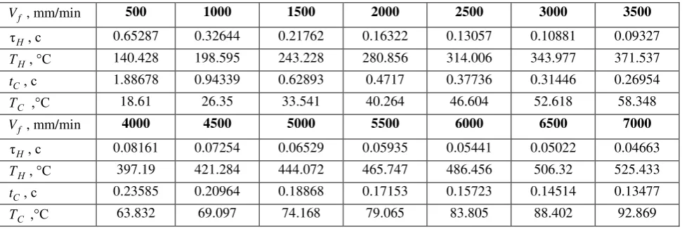
Journal of Engineering Sciences, Volume 5, Issue 1 (2018), pp. A 1–A 7 A 5 Table 2 – Influence of Vf on

τ

, , t , for cycle structure without working stroke omission at tv= 0.074 mm

f

V , mm/min 500 1000 1500 2000 2500 3000 3500

τ , 0.65287 0.32644 0.21762 0.16322 0.13057 0.10881 0.09327

, ° 140.428 198.595 243.228 280.856 314.006 343.977 371.537

t , 1.88678 0.94339 0.62893 0.4717 0.37736 0.31446 0.26954

,° 18.61 26.35 33.541 40.264 46.604 52.618 58.348

f

V , mm/min 4000 4500 5000 5500 6000 6500 7000

τ , 0.08161 0.07254 0.06529 0.05935 0.05441 0.05022 0.04663

, ° 397.19 421.284 444.072 465.747 486.456 506.32 525.433

t , 0.23585 0.20964 0.18868 0.17153 0.15723 0.14514 0.13477

,° 63.832 69.097 74.168 79.065 83.805 88.402 92.869

Table 3 – Influence theVf on thet and for the cycle structure with working stroke omission at tv= 0.015 mm f

V , mm/min 500 1000 1500 2000 2500 3000 3500

t , 9.53357 4.76678 3.17786 2.38339 1.90671 1.58893 1.36194

, ° 12.604 11.976 11.657 11.494 11.426 11.42 11.458

f

V , mm/min 4000 4500 5000 5500 6000 6500 7000

t , 1.1917 1.05929 0.95336 0.86669 0.79446 0.73335 0.68097

, ° 11.529 11.624 11.738 11.867 12.008 12.158 12.317

Table 4 – The same as Table 3 at t_v= 0.074 mm

f

V , mm/min 500 1000 1500 2000 2500 3000 3500

t , 9.53357 4.76678 3.17786 2.38339 1.90671 1.58893 1.36194

, ° 13.57 14.342 15.457 16.726 18.078 19.477 20.902

f

V , mm/min 4000 4500 5000 5500 6000 6500 7000

t , 1.1917 1.05929 0.95336 0.86669 0.79446 0.73335 0.68097

, ° 22.339 23.78 25.218 26.651 28.074 29.487 30.889

Let’s perform a comparison of the cooling tempera-tures for two grinding cycle structempera-tures at tv= 0.015 mm

(Fig. 3, a) and tv= 0,074 mm (Fig. 3, b). There are three

ways to achieve the lowest cooling temperature = 11.6°C for tv= 0,015 mm (Fig. 3, a): 1) when grinding

without working stroke omission with axial feedVf = 0.5

m/min (point A), 2) when grinding with working stroke omission with axial feed Vf =1.8308 m/min (point B,

and 3) the latter at Vf = 4226.9 mm/min (point C).

There are two ways to achieve the lowest cooling tem-perature = 18.6 °C for tv= 0.074 mm (Figure 3 b)

when grinding without working stroke omission with axial feed Vf = 0.5 m/min (point D; 2) when grinding

with working stroke omission with an axial feed

f

V = 2.6444 m/min (point E).

The time to machine by gear grinding both without and with working stroke omission can be determined by the following formulas, respectively

max 1 2

60

IND M

f v

z В l l

T z

V t

 _{ } 

_  _

  ; (7)

max 1 2

2

60

IND

f v

z В l l

T z

V t

 _{ } 

_  _

  , (8)

where B stands for the width of the tooth rim (B =24 mm), z for the number of cogwheel teeth (z = 40), l1 = l2 = 7.86 mm, zmaxfor the grinding stock for machining a cogwheel in the finish (third) stage (z_max= 0,1 mm), INDfor the indexing time (cogwheel

angular turning for one tooth, IND= 4 s).

To ensure the lowest cooling temperature = 11.6 °C, the minimum time to machine is equal to 7.632 min (Table 5) which is obtained in the with work-ing stroke omission cycle structure at tv= 0.015 mm and

f

(6)

A 6 MANUFACTURING ENGINEERING: Machines and Tools

a b

Figure 3 – Cooling temperature vs axial feed Vf for different grinding cycle structures

at tv= 0.015 mm (a) and tv= 0.074 mm (b)

Table 5 – Determining the time to machine in gear grinding Grinding cycle

struc-ture of the

Without working stroke omission

With working stroke omission

The lowest cooling temperature = 11.6 ° at tv= 0.015 mm

Grinding conditions V_f =500 mm/min (point А)

f

V =1830.8 mm/min (point B)

f

V = 4226.9 mm/min (point C)

Time to machine, min 23.852 14.238 7.632

The lowest cooling temperature = 18.6 ° at tv= 0.074 mm

Grinding conditions V_f =500 mm/min (point D)

f

V = 2644.9 mm/min (point E)

Time to machine, min 6.961 4.29

To provide the cooling temperature = 18.6 °C (more than 11.6 °C), the minimum time to machine

M

T = 4.29 min (Table 5) is obtained in the cycle struc-ture with working stroke omission at tv= 0.074 mm and

f

V = 2644.9 mm/min. From these five variants (points A,

B, C, D, and E in Figure 3) we choose the variant with the minimum value = 11.6 °C (points A, B, C), since the theoretical value is = 0. It can be seen (Table 5) that the minimum time to machine TM= 7.632 min is

ob-tained in the cycle structure with working stroke omission at tv = 0.015 mm and Vf = 4226.9 mm/min

( = 11.6 °C).

Thus, the study of the gear grinding temperature mod-els (1) and (3) both at the heating (1) and cooling (3) stages allowed to recommend the working stroke omis-sion in the structure of this operation and to assign the appropriate gear grinding modes for the finish (third) gear grinding stage both for tv = 0.015 mm (points A, B, C in

Figure 3) and tv = 0.074 mm (points D, E).

4 Conclusions

As the depth of gear grinding tvincreases the

maxi-mum cooling temperature increases as well. In the gear grinding cycle structure with working stroke omis-sion cooling time t is greater than that without working stroke omission. As the axial feed Vf increases the

cool-ing temperature for the cycle structure with working stroke omission at tv = 0.015 mm and tv = 0.074 mm

does not practically change, while for the cycle structure without working stroke omission the cooling temperature increases. The smallest cooling temperature is reached at tv = 0,015 mm, so it is expedient to accept the

minimum possible vertical depth of grinding tv on the

finishing (third) gear grinding stage, for example, for the finishing stage we take tv = 0,015 mm.

Moreover, in this stage, the axial feed Vf is chosen

not only from the condition of maximum productivity (maximumVf ), but also from the condition of surface

roughness (in the interval of Vf from 1830.8 to

(7)

Journal of Engineering Sciences, Volume 5, Issue 1 (2018), pp. A 1–A 7 A 7

References

1. Kalashnikov, S. N. et al. (1990). Proizvodstvo zubchatykh koles: Handbook. Moscow, Mashinostroyeniye [in Russian].

2. Lishchenko, N. V. (2016). Opredeleniye intensivnosti zuboshlifovaniya na osnove analiticheskogo uravneniya evol’venty.

Suchasni tekhnologii v mashinobuduvanni, Issue 11 [in Russian].

3. Dekapolitov, M. I. (2011). Povysheniye effektivnosti profil’nogo zuboshlifovaniya tsilindricheskikh koles putem rascheta pa-rametrov staticheskoy naladki: Ph.D. thesis. Specialties 05.02.07 – Tekhnologiya i oborudovanie mekhanich. i fiziko-tekhnologicheskoy obrabotki; 05.02.08 – Tekhnologiya mashinostroyeniya. Moscow.

4. Nishimura, Yu., Katsuma, T., Ashizawa, Y., Yanase, Y., Masuo, K. (2008). Gear grinding processing developed for high-precision gear manufacturing. Mitsubishi Heavy Industries, Ltd. Technical Review, Vol. 45, No. 3, 33–38.

5. Carslaw, H. S., Jaeger, J. C.(1959). Conduction of heat in solids (2nd ed.). London, Oxford University Press.

6. Larshin, V. P. (1999). Tekhnologiya mnogonitochnogo rez’boshlifovaniya pretsizionnykh khodovykh vintov. Proceedings of Odessa National Polytechnic University, Odessa, Issue 2(8), 87–91 [in Russian].