Size Dependence of the Elastic Properties of Pd Nanowire: Molecular Dynamics Simulation

(1)

205 Size Dependence of the Elastic Properties of Pd Nanowire:

Molecular Dynamics Simulation

J. Davoodi

*

_{, M. Ahmadi}

Physics Department, Zanjan University, Zanjan, I.R. Iran

(*) Corresponding author: [email protected]

(Received: 01 Oct. 2010 and Accepted: 20 Dec. 2010)

Abstract:

The mechanical properties including elastic stiffness constants as well as bulk modulus of Palladium (Pd) nanowire were calculated in the constant temperature and pressure (NPT), ensemble by molecular dynamics

(MD) simulation technique. The quantum Sutton-Chen (Q-SC) many-body potential was used to calculate the

cohesive energy as well as forces experience by every atoms. The temperature and pressure of nanowire were

controlled by Nose-Hoover thermostat and Berendsen barostat, respectively. The periodic boundary condition

(PBC) was only applied along the axis of nanowire. The MD results show that the mechanical properties depend on diameter of nanowire. Our results show that elastic constants including C₁₁, C₁₂, C₄₄ and bulk modulus increase nonlinearly with increasing the diameter of nanowire and then reach a constant value, which is a typical behavior of nanoscopic systems.

Keywords: Pd nanowire, Mechanical properties, Molecular Dynamics simulation.

1. INTRODUCTION

A nanowire is an extremely thin wire with a diameter on the order of a few nanometers. The nanowire can be used in nanoelectronic devices and sensors for environmental, medical, etc [1-4]. The Pd nanowire is used extensively in the H₂ gas sensor for its many advantages such as quick response time and operating at room temperature. Therefore, these applications are the motivation for fundamental study of mechanical properties of Pd nanowire. In this study, we focus on the variation of elastic constants including C₁₁, C₁₂, C₄₄, and bulk modulus of Pd nanowire.

The molecular dynamics simulation technique is very powerful tool for studying the physical properties of materials in macro and nano scale. Recently, some MD-based investigations of the thermal and mechanical properties of Pd nanowire have been

carried out [5, 6, 7]. Li Hui et al. were investigated the local atomic structure of Palladium nanowire by molecular dynamics [5]. L. Miro conducted molecular dynamic simulation for thermodynamic and structural properties of Pd cluster and nanowire [6]. Furthermore, melting and structural evolution of bimetallic nanowire including Pd were studied by K. R. S. Sankaranarayanan et al [7]. However, in none of these studies, the effect of diameter size on the elastic constants and bulk modulus were investigated in Pd nanowire. Therefore, in this investigation, we used molecular dynamics simulation technique to study the elastic constants as well as bulk modulus of Pd nanowire. Our simulation applied in constant temperature and pressure ensemble.

(2)

206 Davoodi and Ahmadi

the Pd nanowire. Finally, section four provides our concluding remarks.

2. SIMULATION DETAILS

2.1. Interatomic potential

In the present molecular dynamics simulation

8

Table 1:

The Q-SC potential parameters for Palladium

Metal

ε(eV)

a

(Ǻ)

c n m

Pd 0.003286 3.8813 148.20 12

6

0 1000 2000 3000 4000 5000 6000 7000

-2500 -2000 -1500 -1000 -500 0 500

Time(fs)

Pres

sure

(a

tm)

-3.790 -3.788 -3.786 -3.784 -3.782 -3.780 -3.778 -3.776

Ener

gy

(eV)

Fig. 1

1.5 2.0 2.5 3.0 3.5 4.0 4.5 5.0 5.5

192 194 196 198 200 202 204 206 208

C11

(GP

a)

Diameter (nm)

Fig. 2

1.5 2.0 2.5 3.0 3.5 4.0 4.5 5.0 5.5

128 130 132 134 136 138 140 142 144

C12

(G

Pa)

Diameter (nm)

8

Table 1:

The Q-SC potential parameters for Palladium

Metal

ε

(eV)

a

(

Ǻ

)

c n m

Pd 0.003286 3.8813 148.20 12

6

0 1000 2000 3000 4000 5000 6000 7000

-2500 -2000 -1500 -1000 -500 0 500

Time(fs)

Pres

sure

(a

tm)

-3.790 -3.788 -3.786 -3.784 -3.782 -3.780 -3.778 -3.776

Ener

gy

(eV)

Fig. 1

1.5 2.0 2.5 3.0 3.5 4.0 4.5 5.0 5.5

192 194 196 198 200 202 204 206 208

C11

(GP

a)

Diameter (nm)

Fig. 2

1.5 2.0 2.5 3.0 3.5 4.0 4.5 5.0 5.5

128 130 132 134 136 138 140 142 144

C12

(G

Pa)

Diameter (nm)

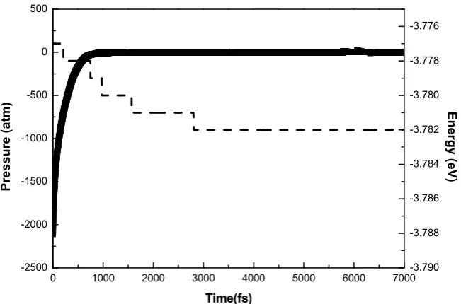
Figure 1: Time variation of the energy and pressure for the Pd nanowire during equilibration

Figure 2: Variation of elastic constant (c11) of Pd nanowire with diameter of nanowire

(3)

207 International Journal of Nanoscience and Nanotechnology

(1)

(2)

3

 



  

 

 



i j i V rij c i

U



( )





2

1 ₍₁₎



 

        

       

i j

m

ij i

n

ij

ij _ra _ra

r

V( ) ,



(2)

The first term, V(rij), describes the pairwise repulsive interaction between atoms i and j, and the

second term, ρi, represents the many-body cohesive term associated with atom i. rij is the distance

between atoms i and j , a is a length parameter scaling, c is a dimensionless parameter scaling, ε sets

the overall energy scale, and n, m are integer parameters. The potential parameters are listed in table

1.

2.2. Temperature control

The extended system method was used for temperature control. This method was originally

introduced by Nose [11] and subsequently developed by Hoover [12], therefore this method was

called Nose-Hoover thermostat. The introduction of this mechanism modifies the standard velocity

Verlet equations of motion [13] to the following forms: [14]

    

  

 

 

 δ () ζ()v()

2 1 ) ( v

δ

) ( )

δ

( 2 _t _t

m t f t t t t r t t

r i

i i i

i i

 

  

    

  

 



 () ζ()v ()

2

δ

) ( v )

δ

2 1 (

v t t

m t f t t t

t i

i i i

i

 

_

  



 _

 





m t gk T

Q t t t

t i b

N i i

) ( v 2

δ

) (

ζ

)

δ

(

ζ 2

2

1  ₍₃₎

   



 _ _

  





m t t gkT

Q t t t t

t i b

N i i

)

δ

( v 2

δ

)

δ

(

ζ

)

δ

(

ζ 2 1₂

2

1 

    

 

 

  

  

i i i

i _m

t t f t t t t t t t

t δ ( δ)

2 1 )

δ

( v )

δ

(

ζ δ

2 2 )

δ

(

v ₂1

 



where Q is given by

2



T gk

Q b (4)

The first term, V(r_ij), describes the pairwise repulsive interaction between atoms i and j, and the second term, ρ_i, represents the many-body cohesive term associated with atom i. r_ij is the distance between atoms i and j , a is a length parameter scaling, c is a dimensionless parameter scaling, ε sets the overall energy scale, and n, m are integer parameters. The potential parameters are listed in table 1.

8

Table 1: The Q-SC potential parameters for Palladium

Metal ε(eV) a(Ǻ) c n m

Pd 0.003286 3.8813 148.20 12 6

0 1000 2000 3000 4000 5000 6000 7000 -2500

-2000 -1500 -1000 -500 0 500

Time(fs)

Pres

sure

(a

tm)

-3.790 -3.788 -3.786 -3.784 -3.782 -3.780 -3.778 -3.776

Ener

gy

(eV)

Fig. 1

1.5 2.0 2.5 3.0 3.5 4.0 4.5 5.0 5.5 192

194 196 198 200 202 204 206 208

C11

(GP

a)

Diameter (nm)

Fig. 2

1.5 2.0 2.5 3.0 3.5 4.0 4.5 5.0 5.5 128

130 132 134 136 138 140 142 144

C12

(G

Pa)

Diameter (nm)

8 Table 1: The Q-SC potential parameters for Palladium

Metal

ε(eV)

a

(Ǻ)

c n m

Pd 0.003286 3.8813 148.20 12

6

0 1000 2000 3000 4000 5000 6000 7000 -2500

-2000 -1500 -1000 -500 0 500

Time(fs)

Pres

sure

(a

tm)

-3.790 -3.788 -3.786 -3.784 -3.782 -3.780 -3.778 -3.776

Ener

gy

(eV)

Fig. 1

1.5 2.0 2.5 3.0 3.5 4.0 4.5 5.0 5.5 192

194 196 198 200 202 204 206 208

C11

(GP

a)

Diameter (nm)

Fig. 2

1.5 2.0 2.5 3.0 3.5 4.0 4.5 5.0 5.5 128

130 132 134 136 138 140 142 144

C12

(G

Pa)

Diameter (nm)

9 Fig. 3

1.5 2.0 2.5 3.0 3.5 4.0 4.5 5.0 5.5 84.0

84.5 85.0 85.5 86.0 86.5 87.0

C44

(G

Pa)

Diameter (nm)

Fig. 4

1.5 2.0 2.5 3.0 3.5 4.0 4.5 5.0 5.5 152

154 156 158 160 162 164

Bu

lk

m

od

ul

us

(G

Pa)

Diameter (nm)

Fig. 5

9 Fig. 3

1.5 2.0 2.5 3.0 3.5 4.0 4.5 5.0 5.5 84.0

84.5 85.0 85.5 86.0 86.5 87.0

C44

(G

Pa)

Diameter (nm)

Fig. 4

1.5 2.0 2.5 3.0 3.5 4.0 4.5 5.0 5.5 152

154 156 158 160 162 164

Bu

lk

m

od

ul

us

(G

Pa)

Diameter (nm)

Fig. 5

Figure 3: Variation of elastic constant (c12) of Pd nanowire with diameter of nanowire

Figure 4: Variation of elastic constant (c44) of Pd

(4)

208 Davoodi and Ahmadi

introduced by Nose [11] and subsequently developed by Hoover [12], therefore this method was called Nose-Hoover thermostat. The introduction of this mechanism modifies the standard velocity Verlet equations of motion [13] to the following forms: [14] (3) 3

 

        

i j i V rij c i

U



( )





2

1 ₍₁₎



                   i j m ij i n ij

ij _ra _ra

r

V( ) ,



(2)

1.

           

 δ () ζ()v ()

2 1 ) ( v δ ) ( ) δ

( 2 _t _t

m t f t t t t r t t r _i i i i i i                

 () ζ()v()

2 δ ) ( v ) δ 2 1 (

v t t

m t f t t t t _i i i i i     _        





m t gk T

Q t t t

t N _i _b

i iv ()

2 δ ) ( ζ ) δ ( ζ 2 2

1  ₍₃₎

          





m t t gkT

Q t t t t

t i b

N i i ) δ ( v 2 δ ) δ ( ζ ) δ (

ζ 2 ₂1

2 1                 i i i i _m t t f t t t t t t t

t δ ( δ)

2 1 ) δ ( v ) δ ( ζ δ 2 2 ) δ (

v ₂1

 



where Q is given by

2



T gk

Q b (4) where Q is given by

3

 

        

i j i ij i

c r V

U



( )





2

1 ₍₁₎



                   i j m ij i n ij

ij _ra _ra

r

V( ) ,



(2)

1.

           

 δ () ζ()v()

2 1 ) ( v δ ) ( ) δ

( 2 _t _t

m t f t t t t r t t r _i i i i i i                

 () ζ()v () 2 δ ) ( v ) δ 2 1 (

v t t

m t f t t t t _i i i i i     _        





m t gk T

Q t t t

t N _i _b

i iv ()

2 δ ) ( ζ ) δ ( ζ 2 2

1  ₍₃₎

          





m t t gkT

Q t t t t

t N _i _b

i iv ( δ)

2 δ ) δ ( ζ ) δ (

ζ 21 2 12

         _       i i i i _m t t f t t t t t t t

t δ ( δ)

2 1 ) δ ( v ) δ ( ζ δ 2 2 ) δ (

v ₂1

 



where Q is given by

2



T gk

Q b (4) (4)

where τ is the relaxation time of the thermostat, and g, the number of freedom of the system is given by g=3(N-1).

2.3. Pressure control

The Berendsen barostat [15] was used to control the pressure of system. This barostat uses a scale factor,

m, which is a function of instantaneous pressure, P, to scale lengths in the system

(5)

4

where τ is the relaxation time of the thermostat, and g, the number of freedom of the system is given

by g=3(N-1).

The Berendsen barostat [15] was used to control the pressure of system. This barostat uses a scale

factor,

μ

, which is a function of instantaneous pressure, P, to scale lengths in the system

L L i z i z i y i y i x i x μ ) ( μ ) ( ) ( μ ) ( ) ( μ ) (     (5)

where

μ

is given by

3 / 1 0) ( δ 1 μ          

 t P P

p



(6)

Here,



pis the rise time of the barostat, δt is the time step and P0 is the set point pressure. The

system pressure is set toward a desired value by changing the dimensions of the simulation cell size

during the simulation.

2.4. Mechanical properties

The quantities which are calculated in this molecular dynamics simulation were the elastic stiffness

constants as well as bulk modulus. The elastic constants reduce to three constants, C11, C12 and C44 for

the cubic crystal by reason of symmetry [16]. In terms of interatomic potential, these quantities can be

expressed as: [17]

2 12 2 44 22 11 2 12 2 11 2 11

4

1

1 





















U

C

U

C

U

C

(7)

where m is given by

4

by g=3(N-1).

factor,

μ

where

μ

is given by

3 / 1 0) ( δ 1 μ          

 t P P

p



(6)

Here,



_pis the rise time of the barostat, δt is the time step and P₀ is the set point pressure. The

expressed as: [17]

2 12 2 44 22 11 2 12 2 11 2 11

4

1

1 





















U

C

U

C

U

C

(7) (6)

Here,

τ

pis the rise time of the barostat, δt is the time

step and

P

0 is the set point pressure. The system

pressure is set toward a desired value by changing the dimensions of the simulation cell size during the simulation.

The quantities which are calculated in this molecular dynamics simulation were the elastic stiffness constants as well as bulk modulus. The elastic constants reduce to three constants, C₁₁, C₁₂ and C₄₄ for the cubic crystal by reason of symmetry [16]. In terms of interatomic potential, these quantities can be expressed as: [17]

(7)

4

by g=3(N-1).

factor,

μ

where

μ

is given by

3 / 1 0) ( δ 1 μ          

 t P P

p



(6)

Here,



pis the rise time of the barostat, δt is the time step and P0 is the set point pressure. The

expressed as: [17]

2 12 2 44 22 11 2 12 2 11 2 11

4

1

1 





















U

C

U

C

U

C

(7)

Where ε₁₁, ε₁₂ and ε₂₂ are the components of strain tensor, Ω is the volume, and U is the energy is given by (1), per atom.

The bulk modulus, which measure how the volume of the solid change with hydrostatic pressure, is denoted by B, which is related to interatomic potential via [17]

0 2 2 Ω = Ω













Ω

∂

Ω

=

U

B

(6)

where Ω₀ is the equilibrium value of Ω.

2.4. Simulation data

(5)

209 International Journal of Nanoscience and Nanotechnology

the diameter of Pd nanowire and calculated mechanical properties, therefore size dependent of mechanical properties of nanowire were obtained. The simulation time step (δt) was set 0.05 fs for every run of MD simulation. The nanowire equilibrated during 200000 time steps in the T=20 K. Figure 1 shows the variation of the energy and pressure in order to detect of the equilibrium state. For translation from macroscale to nanoscale, the periodic boundary condition was only applied in the axis of nanowire and was removed at the other directions. The Berendsen barostat and Nose-Hoover thermostat are used for pressure and temperature control, respectively.

3. RESULTS AND DISCUSSION

The variations of the elastic constants as well as bulk modulus with Pd nanowire diameter were computed in the MD simulation by changing the number of atoms in the nanowire. We have computed cohesive energy for Pd atoms as well, to test the quality of the interatomic potential and our simulation. Our computed results which are shown in the figures 2-5, are in reasonable agreement with other results in the literature where they are available. These results can be fitted into exponential functions. From this figures, it can be seen that there is an initial change in the mechanical properties with the diameter of the nanowire, following which the properties remain unchanged as the nanowire grows in diameter. This is a typical behavior of nanoscopic system in which the mechanical properties, for example, change with size, and then reach a constant value. These results show that, when the diameter of nanowire increase, C₁₁, C₁₂, C₄₄ and bulk modulus will all increase, and when the diameter reach about 5.5 nm, the properties began to level off and remain constant.

Summing up the results of our MD simulations, we see that our molecular dynamics simulation has produced the mechanical properties of Palladium nanowire. The results show that, the mechanical properties depend on diameter nanowire and the

value of elastic constants and bulk modulus of Pd nanowire are different from those properties of bulk Palladium.

REFERENCES

1. A. M. Nicholas, et al., Science 300 (2003)112–115. 2. Y. Huang, X. Duan, and C. M. Lieber, Nanophotonic

assemblies 1 1 (2005) 142-147.

3. Y. Wu, R. Fan, P. Yang, NANO LETTERS 2 (2002) 83-86.

4. H. Yan, S.H. Park, G. Finkelstein, J.H. Reif, T.H. LaBean, Science 301(2003) 1882-1884.

5. L. Hui, B. L. Wang, J. L. Wang, and G. H. Wang, J.

Chem. Phys., 121 (2004) 8990-8996.

6. L. Miao, V. R. Bhethanabotla, B. Joseph, PHYSICAL

REVIEW B 72 (2005) 134109.

7. S. Sankranarayanan, V. R. Bhethanabotle, B.

Joeseph, Journal of physical chemistry. C 111 (2007) 2430-2439.

8. A. P. Sutton, J. Chen, Philosophical Magazine

Letters 61 (1990) 139– 164.

9. J. Davoodi, M. Ahmadi, Computational Materials

Science 49 (2010) 21–24.

10. J. Davoodi, M. Ahmadi, H. Rafii-Tabar, Materials

Science and Engineering A 527 (2010) 4008–4013. 11. S. Nose, J. Chem. Phys. 81 (1984) 511-519.

12. W. G. Hoover, Phys. Rev. A 31 (1985) 1695-1697.

13. D. Frenkel, B. Smit, Understanding molecular

simulation from algorithms to application, Academic press, New York, (2002).

14. A. P. Sutton, J.B. Ptthica, H. Rafii-Tabar, J.A. Nieminen, in: d. G. Pettifor, A.H. Cottrell (Eds.), Electron Theory in Alloy Design, Institute of

Materials, London, (1994) 191.

15. H. J. C. Berendsen, J. P. M. Postma, W. F. van Gunsteren, A. DiNola, and J. R. Haak, J. Chem. Phys. 81 (1984)3684-3690.

16. C. Kittel, Introduction to Solid State Physics, eighth ed., John Wiley & Sons, New York, (2005).