R E S E A R C H
Open Access
Estimating the savings potential of
occupancy-based heating strategies
Vincent Becker
*, Wilhelm Kleiminger
, Vlad C. Coroam˘a
and Friedemann Mattern
FromThe 7th DACH+ Conference on Energy Informatics Oldenburg, Germany. 11-12 October 2018
*Correspondence: [email protected] Department of Computer Science, ETH Zurich, Universitätstrasse 6, 8092 Zurich, Switzerland
Abstract
Because space heating causes a large fraction of energy consumed in households, occupancy-based heating systems have become more and more popular in recent years. However, there is still no practical method to estimate the potential energy savings before installing such a system. While substantial work has been done on occupancy detection, previous work does not address a combination with heating simulation in order to provide an easily applicable method to estimate this savings potential. In this paper we present such a combination of an occupancy detection algorithm based on smart electricity meter data and a building heating simulation, which only requires publicly available weather data and some relevant building characteristics. We apply our method to a dataset containing such data for several thousand households and show that when taking occupancy into account, a
household can save over 9% heating energy on average, while certain groups, such as employed single-person households, can even save 14% on average. Using our approach, households with high potential for energy savings can be quickly identified and their inhabitants could be more easily convinced to adopt an occupancy-based heating strategy.
Keywords: Smart heating, Occupancy detection, Household heating simulation, Energy savings, Smart energy
Introduction
Space heating is the main factor driving the energy consumption of households. Studies show that it dominates the energy consumption of households in the European Union (EU) with 67% of the total energy use (Lapillonne et al. 2015). The residential sec-tor overall accounts for 25% of the final energy consumption, comparable to the EU’s entire industry sector (Eurostat2018). Other countries report similarly significant num-bers (International Energy Agency2015). Space heating in households thus bears great potential for energy savings, leading to both financial and environmental benefits.
One way to decrease the amount of heating energy is to use a heating strategy based on the occupancy of the dwelling: when a building is unoccupied, the heating is turned down. Such a strategy could be carried out in different ways. The inhabitants could simply take care to turn down the temperature themselves whenever they leave. Nowadays, this
is becoming easier due to heating systems which can be controlled remotely via smart-phone apps; however, the inhabitants still have to explicitly remember and take action themselves on a daily basis. Alternatively, heating systems that automatically detect the occupancy of a dwelling are slowly gaining interest and are being increasingly used in households (Markit2015; U.S. Department of Energy2016).
The savings that occupancy-based heating can achieve, however, depend on numerous parameters such as building size and insulation, climate, and in particular the occu-pancy schedule of inhabitants. Given the large variation – and thus the uncertainty – of achievable savings, home owners and tenants are understandably reluctant to install smart heating systems. In this paper, we address this uncertainty by introducing a novel method that quickly estimates the savings potential of a household. The method builds upon previous work on non-intrusive occupancy detection (Becker and Kleiminger2018), combining it with a heating simulation. The occupancy detection relies on smart meter data and derives the occupancy schedule from the observed electricity consumption. This schedule serves as input to the simulation, which additionally takes weather data and a few relevant building parameters into account. If a dwelling is already equipped with a smart electricity meter, all data is easily available. The simulation of the household’s heating is then adapted to the derived occupancy schedule, subsequently calculating the potential savings as shown in Section “Method description”.
Not relying on special equipment, our method is suitable for any household equipped with a smart meter. It can be used to easily estimate the energy saving potential of occupancy-based smart heating for a given household. Additionally, the method read-ily scales. Statistical data on buildings’ characteristics in an area provided, it could be deployed by e.g. municipalities to identify the households with highest poten-tial for energy savings in their territory, and target their energy efficiency measures accordingly.
Related work
In the following we discuss different categories of related work aiming at saving heating energy in households. We will not discuss occupancy detection, however, as our method we build upon here is examined in (Becker and Kleiminger 2018) and overviews on building occupancy estimation are available in the literature (Chen et al.2018).
Smart heating
Many energy saving measures for households target electrical appliances. However, with a proportion of about 67% of the total energy consumption in Europe (Lapillonne et al.
2015) and regions with a similar climate, heating (or, in a more general sense, HVAC: Heating, Ventilation, and Air Conditioning) has a much greater impact on the total energy consumption of a household. Approaches to decrease the heating energy of dwellings can be separated into two categories: infrastructural approaches (e.g. retro-fit insulation) and control measures (e.g. optimising the heating schedule).
smartphone (e.g. Heat Genius Ltd2018), so they can turn it off while they are not at home, and back on again before they return in order to heat the home prior to arrival.
More complex systems detect or even predict the occupancy of the inhabitants to control the heating, for example by tracking the inhabitants’ smartphone locations and thereby estimating their arrival in order to preheat the dwelling. Complementarily, they might also employ motion sensors to detect the occupancy of individual rooms and heat them as needed. Some of the commercial systems mentioned above exhibit such char-acteristics (Tado2018; Heatmiser2018; Heat Genius Ltd2018). Furthermore, there are systems which try to learn the preferences of the inhabitants and apply these after a learn-ing period. One of the more prominent systems is the Nest thermostat (Nest2018). As they automatically (at least after a certain training time) and autonomously control the heating, these are typical instances of what is usually referred to assmart heating.
Occupancy-based building energy estimations
Using occupancy to estimate heating energy consumption has recently been pursued by several researchers. Erickson et al. (2013) deploy a camera and passive infrared (PIR) sen-sor network in an office and lab building. Features from both are fused using a particle filter to detect occupancy. A Markov chain is then employed for occupancy prediction in order to control the HVAC system. The savings are estimated both for a live deployment in the building, as well as using a simulation model. The authors estimate savings for heat-ing, coolheat-ing, and ventilation of up to 30%. In contrast to our system that only relies on smart meters, the suggested method requires dedicated hardware, typically not available in homes. Next to the costs for purchase, installation, and maintenance, this means above all that the system does not scale well. The result was obtained for a particular office build-ing in California where more energy is used for coolbuild-ing and ventilation than for heatbuild-ing, and where parts of the building (meeting rooms and some offices) have a low occupancy rate. Hence, it does not apply to the heating of residential households which is the focus of this paper.
Kim et al. (2017) employ linear regression based on electricity use data to estimate the number of occupants in a building in order to calibrate energy building models to improve the prediction of building energy consumption. Their system is evaluated on data from an office and two campus buildings. Our approach differs in several ways: we apply our system to residential households, which have a less regular schedule, use a sim-ulation model to predict heating energy consumption, and finally we are able to calculate potential savings by comparing different heating strategies.
estimation algorithm based only on the electricity consumption available through smart meters. Furthermore, we use a generic model which requires only the provision of a few characteristic parameters regarding the dwelling and the local weather conditions. Thus, our approach is immediately applicable to a large variety of households, and could directly be used in a real-world setting.
Kruusimägi et al. (2018) create an occupancy-based heating control system for an elec-tric heater in residential homes using simple hardware and a relatively simple prediction approach. Furthermore, the inhabitants can interact with the system via a smartphone app to rate their current comfort and enter irregular absences. To evaluate their system, the authors employ a simulation and run it in three real households. In the simulation they find significant energy savings when comparing to a standard fixed heating schedule. Their evaluation step using the simulation appears similar to our approach, however, the goals are different. While Kruusimagi et al.2018evaluate the savings when employing its predictive heating system in specific model households, we intend to provide a method which in general estimates the potential of such a system for any household and answers the question whether its use seems reasonable.
Method description
Our aim is to estimate the potential heating energy savings of a dwelling for a period in the past if an occupancy-based heating strategy had been applied, e.g. for the past year. We first learn the occupancy pattern in that period from a household’s electricity con-sumption and then simulate its thermal energy concon-sumption optimised to this particular occupancy pattern. The essential concept of our approach is the combination of these two components, automatic occupancy detection and the heating simulation, as illus-trated in Fig.1. Both parts have been explored separately in previous works (Becker and Kleiminger2018; Kleiminger et al.2014a,b), but only by integrating them, one obtains a system toautomaticallyestimate the savings potential of a particular household or to cal-culate statistics from a large set of household and building data. The calculations rely on four sets of parameters:
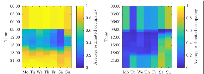
(1) Occupancy. The heating simulation requires the occupancy schedule, i.e. a timeline when the home is occupied or unoccupied, which is computed prior to the simulation. The lower the occupancy, the higher the potential savings, since the heating could be turned down in times of absence. As an example for the importance of the latter, Fig.2
Fig. 1An overview of our approach to determine the savings potential with inputs marked in red
activities (i.e. use of appliances) in the household. At the same time, smart meters, which continuously measure the electrical power consumption of a household, are becoming increasingly ubiquitous (cf. U.S. Energy Information Administration (EIA)2017, Table 10.10 and European Commission2014a) – a penetration rate of 95% is expected in sixteen EU member countries by 2020 (European Commission2014b).
(2) Characteristics of the dwelling. The amount of heating energy used strongly depends on the characteristics of the dwelling, such as how well insulated and how large it is. Heating an unoccupied dwelling consumes more energy if its insulation is poor, hence the potential savings are high in such cases.
(3) Weather. We take the local weather into account. In cold climates, it takes longer to re-heat an unoccupied building, which affects the savings potential.
(4) Heating strategy. We distinguish different heating strategies, which influence the way the dwelling is heated in the simulation environment. Since we are performing an offline analysis of the potential benefits of smart heating systems and are working with historical data taking an a-posteriori view, the simulated heating controller can take advantage of perfect knowledge of future occupancy and weather conditions. Because the time it takes to re-heat a house after it has cooled down is non-negligible, the so-called
oracle strategytakes future occupancy and weather into account in order to preheat the dwelling before the residents return and thus to avoid comfort loss. While an ideal ora-cle policy is adequate for an offline analysis of the savings potential (as in our case), a controller driving an actual heating system based on occupancy prediction requires an online prediction algorithm in practice. An analysis of the effects of various online pre-diction algorithms on the achievable savings with respect to the oracle strategy is given in (Kleiminger et al.2014a), where the authors show that with a suitable prediction algo-rithm the theoretical oracle strategy can be approximated with a prediction accuracy of over 80% and negligible comfort reduction. Thus, a good approximation of the oracle strategy can indeed be implemented in a real-world space heating system.
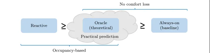
Two extreme strategies,reactiveandalways-on, are useful for the analysis of the saving potential, as they represent boundary cases: Thereactive strategyuses no future informa-tion and only heats the dwelling when it is occupied; in particular, it does not preheat the dwelling in anticipation of the inhabitants’ return. Hence, in a real-world application it would only require occupancy detection, and no prediction. The energy required for heat-ing is at most the demand of the oracle strategy (in the case the home is always occupied) but typically less. Since there may be a comfort loss as the dwelling is not heated before the residents actually return, one would in practice augment the reactive strategy with a remote control for preheating (e.g. via an app). Additionally, we consider analways-on strategy, which assumes the home is occupied all the time. This is equivalent to a fixed setpoint operation mode. We use it as a baseline, to which we compare the occupancy-based strategies. The occupancy-occupancy-based strategies should use significantly less energy than thealways-on strategy. Figure3summarises the relationship of the three strategies.
Our approach can thus be summarised as follows: Based on a household’s auto-matically determined occupancy schedule, the characteristics of the dwelling, and the
environmental conditions, we compute the required heating energy of the three strate-gies (oracle, reactive, always-on) by controlling the temperature of the simulated building using the occupancy schedule. The savings are calculated by comparing the results of the occupancy-based strategies (oracle and reactive) to the always-on base-case strategy.
Occupancy detection
We briefly explain the applied occupancy detection algorithm, but refer the reader to the relevant publication (Becker and Kleiminger2018) for more details. The input consists of sequences of electricity consumption samples. Here, each sample is the mean consump-tion in a 30 min time slot as delivered by a typical smart meter. The core of the process is a Hidden Markov Model (HMM), which is used for classification, i.e. making a decision for each time slot about the occupancy state based on the electricity consumption. Since the occupancy is binary, the model only has two states. The resulting sequence of occu-pancy states is the schedule used as input to the simulation model. Note that we take an a-posteriori view, i.e. the model can take all the available data into account when classify-ing a sample. The parameters of the HMM are estimated from the available data and not trained in a supervised manner to be able to handle data without an occupancy ground truth as in our case.
An extra step is added to infer the occupancy at night. Since during sleep people do not interact with electrical devices and most of them are turned off or in standby mode, it is difficult to obtain occupancy information from the electricity consumption. A nightly schedule is added using the following simple heuristic: If the dwelling is occupied for at least one hour from 8 p.m. to midnight, we count the whole night (until 9 a.m.) as occupied. If more information on the occupants specific schedule, such as working night shifts, was available, this could also be taken into account.
The algorithm was validated on three datasets containing ground truth and achieved an average accuracy of 83%. We believe this is high enough for our purpose of estimating the heating savings. A sensitivity analysis on how the estimation reacts to changes in the occupancy is given in Subsection “Sensitivity to the occupancy estimation”.
Household heating simulation
20°C for living areas and a temperature of 15 - 18°C for hallways and bedrooms (Sus-tainable Energy Authority of Ireland2018). Similarly, the German Federal Environmental Office advises to set the temperature to 20° - 22°C for the living room, 18°C for the kitchen and 17° - 18°C for the bedroom (Umweltbundesamt2017). For periods of absence the temperature should be reduced to 18°C, to 15°C in case of an absence of a few days, or even lower for longer periods of absence. Hence we think that the default temperature values we choose for comfort and setback are reasonable. Note that a setback tempera-ture of 10°C would only be reached after long periods of absence in winter, which are rare. Other temperature settings and an analysis of the sensitivity to different settings will be discussed in Subsection “Sensitivity to the thermostat settings”.
As the heating simulation requires the weather data and also building information for the particular households, we explain how we obtain this data for the set of our test house-holds in Subsection “The CER dataset”. Note, however, that our approach is not specific to households in a certain dataset, but can be applied to any household for which the necessary parameters are available.
Savings potential evaluation
In order to demonstrate our system and gather insights about possible saving potentials when employing an occupancy-based heating regime, we apply it to a large dataset con-taining smart meter data and relevant household characteristics. We use the CER dataset from the Irish Commission for Energy Regulation, which is further described in the fol-lowing subsection. As the CER dataset contains no occupancy ground truth, we cannot verify the calculated occupancy values and rely on the algorithm’s validation carried out in previous work (Becker and Kleiminger2018). After applying our method to each house-hold in the CER dataset and retrieving the potential savings for each of them, we analyse the savings by groups, such as singles versus families, since we expect significant differ-ences between them. Furthermore, we examine characteristic properties of households with higher and lower potential savings, respectively.
The CER dataset
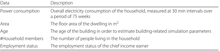
The CER dataset (Irish Social Science Data Archive2018) contains the power consump-tion data for over 4,000 households and small businesses in Ireland. The data we use consists of 75 weeks’ worth of electricity consumption data measured at intervals of 30 min from July 2009 to December 2010. Additionally, the households participated in a survey in which they had to answer questionnaires in order to assess their personal cir-cumstances and characteristics of their home. Table1shows all the data from the CER dataset we used for the occupancy schedules, the simulation, and the savings estimation.
Table 1The data from the CER dataset relevant for our savings analysis
Data Description
Power consumption Overall electricity consumption of the household, measured at 30 min intervals over a period of 75 weeks
Area The floor area of the dwelling inm2
Age The age of the building in order to estimate building-related simulation parameters #Household members The number of people living in the household
We remove all households for which the age of the building (which determines the building-related parameters) is missing, and also all households for which there were at least ten missing electricity consumption values a day on at least 10 days (e.g. due to smart meter malfunctioning). The final set contains 3,476 households. The data for our analysis consists only of the electricity load data and the basic information about the household (cf. Table1). A thorough analysis on more household characteristics and their classification from electricity data can be found in (Beckel2016).
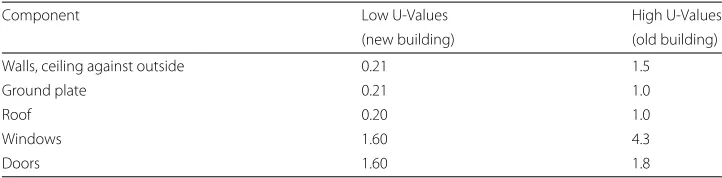
Two characteristics of a household are especially important for our heating simulation, namely the age of the building and the floor area. We use the age to estimate the insulation quality of a dwelling. The insulation of a building element is usually given by its U-value, which expresses its heat transfer coefficient measured in W/m2K. For example, a build-ing which has a roof with a high U-value will thus lose a significant amount of energy through the roof. For Ireland, appropriate values can be found in the Technical Guidance Document L of the Irish Building Regulations (Irish Department of Housing Planning, Community and Local Government2017). Regarding the U-values, we create two sets of parameters, one for “old” and one for “new” buildings. We divide the households into two sets of equal cardinality and therefore consider all buildings built before 1980 as “old”, all the others as “new”. According to this, 49.97% of the relevant buildings in the dataset are considered old. For new buildings we use the U-values from the Irish Buildings Regula-tion. For old buildings we use a list of high U-values for poor insulations from (Wikipedia
2018). Table2shows the U-values for the old and new buildings, respectively.
The size of the dwelling affects the heating energy consumption as well; the larger the dwelling, the more heating energy is consumed. The floor area of the buildings is derived from the CER dataset. Since we do not know the exact geometry of the buildings, we assume that they have a square floor shape. Each of these buildings is given a total window area of 25%, the default value as noted in the Irish building regulations (Irish Department of Housing Planning, Community and Local Government2017) (we note in passing that while the window size has an important influence on the absolute heating energy demand, we found that it is a negligible parameter when determining therelativesavings of an occupancy-based strategy compared to the always-on base case). As in the previous work, the design heat load (maximum heating power) of the heating system was determined according to the European standard EN 12831 (DIN2008).
The temperature and solar radiation data for the period from July 2009 to December 2010 for Ireland were obtained from Met Éireann (The Irish Metrological Service Online
2018). Since the exact location of the buildings associated with the metering data was not available, we used the data for Dublin Airport. The temperature and solar radiation data were interpolated from hourly measurements to 30 min measurements.
Table 2U-valuesW/m2K
Component Low U-Values High U-Values
(new building) (old building)
Walls, ceiling against outside 0.21 1.5
Ground plate 0.21 1.0
Roof 0.20 1.0
Windows 1.60 4.3
We note that after running the occupancy detection algorithm on the CER dataset, we observed an average estimated occupancy of 75.4%, which matches the rate of 73.6% reported in the Irish national time use survey quite closely (McGinnity et al.2005).
Savings calculations
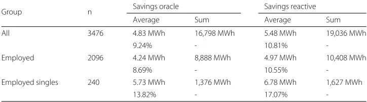
From the heating simulation results we calculate the absolute and relative savings. We calculate the savings for three different groups: all of the households, those in which the chief income earner is employed, and those in which only a single person lives, who is also employed. In the households we examined, 60.3% of the chief income earners were employed or self-employed (which we count as employed). The reason why these groups are interesting, is that we expect these characteristics to have a significant influence on the occupancy and consequently also on the savings.
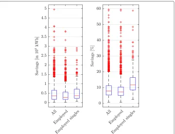
As explained in Section “Method description”, the savings we present here are the dif-ference between the occupancy-based heating strategies, i.e. oracle and reactive on the one side, and the always-on strategy as the base case on the other side. For each of the occupancy-based strategies and the groups of households we show the mean and the sum of absolute and relative savings over the full trial time of 75 weeks. The absolute savings are savings in usable heating energy (i.e. the output of the heating system and not the input). The resulting savings are shown in Table3and in Fig.4. Since the results of the oracle and the reactive strategies do not differ much (cf. Table3) and since the oracle is the more appropriate strategy for a smart heating system due to the lower comfort loss, we mainly comment on the oracle results below, although the main conclusions apply to both strategies and in particular to possible practical approaches using prediction algorithms (Kleiminger et al.2014a) which approximate an oracle occupancy schedule. Over all 3,476 households, we observe that on average over 9% energy could be saved in heating using the oracle strategy (cf. Table3; remarkably, this corresponds to the savings determined for an exemplary scenario in Switzerland in Kleiminger et al.2014). As we expected, we find the highest average savings for the employed singles with nearly 14% savings, since they are usually at work during daytime and consequently the home is unoccupied for longer periods of time. These numbers show that applying occupancy-based strategies could greatly contribute to reaching energy efficiency goals (cf. Section “Introduction”). Moreover, such strategies can create financial benefits for households.
Identifying households with high savings potential
Figure5 depicts the histogram of the relative savings for the oracle strategy. Over all households the peak of the distribution is below 10%. Nevertheless, there are households
Table 3The savings for each group over the period of 75 weeks. The numbers are rounded to two decimals or zero decimals for large values
Group n Savings oracle Savings reactive
Average Sum Average Sum
All 3476 4.83 MWh 16,798 MWh 5.48 MWh 19,036 MWh
9.24% - 10.81%
-Employed 2096 4.24 MWh 8,888 MWh 4.97 MWh 10,408 MWh
8.69% - 10.55%
-Employed singles 240 5.73 MWh 1,376 MWh 6.78 MWh 1,627 MWh
-Fig. 4The absolute savings in kWh and relative savings in % for each group for the oracle strategy over the period of 75 weeks
which can save over 15%. As mentioned in our initial motivation, one crucial contribution of our approach is that we can quantify the savings for individual households and thereby quickly identify households with a high savings potential for which changes in their heat-ing behaviour make sense. In the dataset, 409 households (11.8%) could save at least 15% and 180 of them (5.2%) could even save at least 20% (which are shown as red crosses in the right plot of Fig.4). The high savings for these households could help to convince the residents to act upon their heating energy consumption, either by investing in a smart heating system or changing their habits.
We examine which characteristics explain the high saving potentials of these house-holds. Figure6shows a comparison between all households, employed households, and the 180 outliers (which would save at least 20%) for six different characteristics. We find clear differences in four characteristics: the proportion of employed singles, old dwellings, the average duration of absence, and the number of people per dwelling. As mentioned in Section “Method description”, for old buildings the savings are higher. Interestingly, the average occupancy is nearly the same for all the groups. However, there are great dif-ferences in the average duration of continuous periods of absence. More energy can be saved for long periods of absence since then the house does not have to be heated for a long time and has to be reheated only once. If the occupancy state changed several times per day, the dwelling would have to be heated even during short absences to be preheated for the frequent occupied time slots. The length of these periods naturally correlates with the number of people in a household, i.e. long average periods of absence are an effect of only few people living in a household. As the group of employed people have the highest average number of people per dwelling, this also explains why they have lower savings (cf. Table3).
Model assumptions and sensitivity analysis
We now discuss and justify some of our assumptions, and analyse the stability and robustness of our method and results.
Nightly setback
Often, households have a timer-driven heating system which lets the temperature drop to a certain setback temperature at night in order to save energy. One could argue that for our analysis a baseline in which the temperature is decreased during the night makes more sense than the always-on baseline. However, if we used a baseline with a night-time setback temperature, we could also use this setback in the occupancy-based
strategies, which then consequently would also use less energy (because at night a home is typically occupied). For the setting with a nightly setback the savings are even higher (6.64 MWh on average for the oracle strategy compared to 4.83 MWh over the 75 weeks period). This is due to the possibility of obtaining schedules with very long peri-ods of absence, e.g. when the dwelling is unoccupied the whole day, it does not have to be heated above the setback temperature for the previous night and that day. This effect is naturally even stronger for reactive schedules (8.41 MWh instead of 5.48 MWh energy savings).
Heating simulation model
For the heating simulation, we use a standardised (ISO 13790), but relatively simple 5R1C household heating model and additionally make some assumptions on the building, such as the insulation characteristics, based on the year of construction. There are more sophisticated and exact heating models available, which however require more detailed information on each household and building. If this information is available, the 5R1C model could be replaced by the more complex model without defying the purpose of our method. For large-scale evaluations of several thousand households, such as the CER dataset, this information is typically not available and hence more sophisticated models are no viable option.
The simple model used in our evaluation might induce modelling errors in the estimated heating energy. However, for each household the error will most likely persist in all the strategies and have a similar value. Since we are only interested in the difference between the strategies, the errors will largely coun-terbalance each other, the resulting error in the savings estimate thus being mitigated.
Sensitivity to the occupancy estimation
Errors in the detection or prediction may impair the savings potential when the false positive rate is high, i.e. the dwelling is heated when nobody is at home. The comfort may suffer from false-negatives, i.e. the dwelling is not heated or the temperature is not yet high enough when the home is in fact occupied. However, in a real-world deploy-ment there are several possibilities for technical measures to counteract this comfort loss, e.g. an “override” button inside the home or a smartphone app to overrule the automatic heating control. The discussion of these means is out of the scope of this paper.
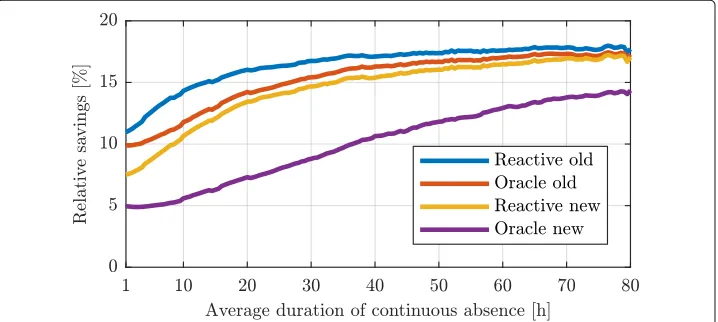
As our simulation and as such our savings estimation depend on the output of the occu-pancy detection, we might be facing second-order errors in the savings estimation due to errors in the occupancy detection. Since we have no occupancy ground truth for the CER dataset, we cannot directly validate our occupancy detection results. We acknowl-edge that potentially there are errors in the detection, but the question is how strongly the savings results react to errors in the occupancy detection: If the detection makes only a few more errors, are the savings affected only a little, too, or possibly a lot? To address this question, we simulate artificial households: one “new” and one “old” building with a floor area of 149m2each, the mean in the CER dataset. We vary the occupancypatternto examine how the savings are influenced by the changes. For a specific duration of contin-uous absence we create artificial schedules which all have an average occupancy of 75% (the average in the CER dataset), but different absence patterns. For example, for a period of absence of two hours, we set the first four 30 min slots tounoccupiedand the following twelve slots tooccupied, then the next four tounoccupiedagain and so on. Figure7shows how the relative savings increase as the duration of absence increases. This is because for longer absences the dwelling has to be pre-heated less often. The curves show that small changes only have a small impact and thus few errors in the occupancy detection will only have a minor influence on the results. The interdependence of energy savings, discomfort due to prediction errors, and occupancy estimation performance is explored in greater detail in (Gluck et al.2017).
Fig. 7The relative savings for two artificial households (one “new” and one “old”) depending on the duration of continuous absence. The average occupancy always is 75%. Since in any case the household is
Sensitivity to the thermostat settings
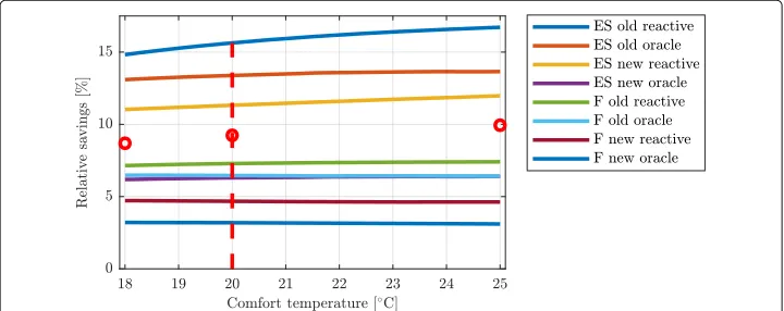
Another interesting point is to examine how the savings depend on the temperature set-tings. Our simulation has two temperature parameters, the comfort temperature, which is the target to be reached when the dwelling is occupied, and the setback temperature, the value to which the temperature is allowed to drop when the dwelling is unoccupied. A low setback temperature is important to benefit from longer absences (in particular for old houses with poor insulation). While the overall savings for a setback temperature of 10°C are 9.2% for the oracle strategy (cf. Section “Savings potential evaluation”), they drop to 7.6% if we let the setback temperature increase to 15°C. Similarly, the comfort temperature has a significant influence on how much energy is consumed for heating. Applying an occupancy-based heating strategy, theabsolutesavings will be higher when the comfort temperature is increased due to saving the greater amount of energy required for heating to higher temperatures. The question is how strongly this affects the rela-tivesavings, i.e. the ratio of estimated absolute savings and absolute consumption for the “always-on” baseline strategy. To explore this, we run simulations for two artificial but typical schedules, “employed singles” and “family”, varying the comfort temperature. In the “employed singles” schedule, the dwelling is unoccupied from 9 a.m. to 6 p.m. from Monday to Friday, and from 8 p.m. to 11 p.m. on Fridays and Saturdays. In the “family” schedule, the dwelling is unoccupied from 9 a.m. to 2 p.m. Monday to Friday. Additionally, for each schedule we simulate a “new” and an “old” dwelling, i.e. we obtain four artificial households. The comfort temperature is varied from 18°C to 25°C in steps of a quar-ter of a degree. The range corresponds to advice on temperature settings for households published by the Sustainable Energy Authority of Ireland (2018) and the German Fed-eral Environmental Office (Umweltbundesamt2017). The results are depicted in Fig.8. It shows that the relative savings only slightly increase when increasing the comfort tem-perature. This effect is strongest for the “employed singles” setting with an “old” dwelling and employing the reactive strategy – however the increase is still less than two percent points over the full range. For the “family” setting the relative savings are nearly constant. As usual, the savings are smaller for the oracle strategy than for the reactive strategy, but
also the increase in savings is less. This is due to a contrary effect for the oracle strat-egy: the higher the comfort temperature, the earlier the household has to be preheated in periods of absence.
Additionally, we ran the simulation for the whole dataset again for the extremes of the examined comfort temperature range, which are marked as red circles in Fig.8. The aver-age relative savings for all households at comfort temperatures of 18°C and 25°C were 8.69% and 9.94%, respectively. The values show little deviation from the savings at a com-fort temperature of 20°C (9.24%, cf. Table3) which we used for evaluation. Overall, we find that the relative savings results for the chosen comfort temperature of 20°C are also valid for other reasonable temperature settings.
Sensitivity to the heating power
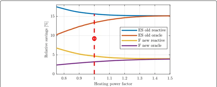
In our analysis, we determined the maximum power the heating system of a dwelling is able to deliver (the so-called design heat load) according to the European standard EN 12831. One can expect, however, that in practice a particular heating system deviates in one way or the other from that standard. For occupancy-based heating regimes, the available heating power is indeed an important aspect to consider. We perform similar simulations as in the previous subsection, using the same artificial households. Instead of altering the comfort temperature (which is set to its default value of 20°C here), we scale the design heat load by a scalar, the heating power factor. We vary it in a reasonable range from 0.75 to 1.5. For these values, the total energy consumed for the always-on strategy (our baseline and the denominator in the calculation of the relative savings) is almost con-stant. A heating power factor of one results in our default design heat load value. Figure9
shows the results for two of the artificial households with both heating strategies. For the other household types, the conclusions are similar. The higher the design heat load, the shorter the period a dwelling has to be preheated before the arrival of the inhabi-tants when employing the oracle strategy. Therefore, the savings are higher with a more powerful heating system. For the reactive strategy the opposite is the case, however. The reactive strategy only heats the dwelling upon arrival, however then it will try to heat it up
as quickly as possible with all the heating power available, if necessary, as its primary con-cern is to minimise the comfort loss of the inhabitants. That means, with a higher heating power, the comfort will be higher, but also the amount of energy consumed. Overall, the gap between the oracle and the reactive strategy shrinks with an increasing design heat load.
Discussion
Behavioural, economic, and societal effects
The savings potential discussed in Subsection “Savings calculations” will not be fully exploited in practice because of some known adverse effects. For example, the accep-tance of “smart” technology is never at 100%, and some inhabitants would not be willing to accept an even moderately reduced comfort resulting from prediction errors, or they might suspect discomfort for their cherished pets left behind alone at home. Further-more, the inhabitants’ anticipation of energy savings may lead to an adverse behavioural response due to the rebound effect, a known problem in energy economics (Greening et al.2000; Sorrell2007). The energy and cost savings resulting from a smart heating system might be seen as a reason to increase the temperature of the dwelling, or to buy newer or larger devices. The subsequent increases in energy consumption might reduce or even overcompensate the initial savings of the smart heating. Furthermore, saving energy in one’s household may lead people to believe they have reached the moral high ground in terms of energy savings and relieve their conscience with regard to energy conservation in other areas of their daily life, e.g. when driving an energy-inefficient car – a behaviour known as moral licensing (Sachdeva et al.2009; Merritt et al.2010). Such behavioural and economic effects and their impact on the effective energy savings are important but difficult to estimate, and their analysis is beyond the scope of this paper.
As shown, we estimate high relative saving potential for employed singles. The largest absolute savings are reached for working singles who inhabit large homes, ideally poorly insulated. This raises questions of social justice and equity: should possible public fund-ing or subsidies for smart heatfund-ing systems be used in aidfund-ing poorer families, inhabitfund-ing relatively small homes and who are possibly unemployed, the rather small environmental effect notwithstanding? Or should the households with the largest environmental impact be targeted, despite the fact that working singles who live in large mansions are not tra-ditional targets of social subsidies? This sustainability dilemma can only be addressed by a broad policy dialogue. It lies outside the scope of this paper, which can only inform the political and societal debate.
A “future-proof issue”?
Will the saving of energy for space heating still be a relevant issue in the medium- to long-term future? After all, steady efficiency improvements with building envelope technolo-gies (better insulation, lower U-Values, etc.), but also global warming should gradually reduce the problem. In fact, Connolly conjectures that due to technical improvements to be expected in the coming decades, heat demand in the EU buildings sector could eventually be halved (Connolly2017). Additional savings beyond that, however, would be uneconomical, he believes.
driving up demand for space heating energy. In the UK, for example, average indoor temperatures have risen steadily over the past 40 years, from 13°C in the late 1970ies to around 17.5°C now (cf. Department for Business, Energy & Industrial Strategy, UK
2017, Table 3.16). Johnston et al. (2005) assume that if the standard of living contin-ues to rise, the mean internal temperature of UK dwellings will saturate at around 21°C by 2040 or 2050.
Secondly, while today households in the EU use on average less than 1% of their energy for cooling (Lapillonne et al.2015), and a lot of building space in Europe is not cooled at all, Werner notes that for an ideal indoor climate many buildings should indeed be cooled (Werner2016). The general consensus is that cooling needs will increase as com-fort levels improve in the coming decades. To meet all the cooling needs, Werner expects a sixfold increase in the cooling demands in the EU compared to today. And while global warming by 1° to 2°C over the next decades might reduce the demand for heating energy, it would conversely drive up electricity demand for cooling purposes. It should be clear that the technologies for occupancy-based space heating presented in this paper can in principle also be used in occupancy-based cooling schemes (or HVAC control systems in general) to save energy and cost (Gluck et al.2017). Aftab et al. (2017) recently pro-posed an occupancy-based HVAC control system to save energy when cooling mosques. Peng et al. (2018) examined the use of an occupancy-prediction-based cooling system in an office building in Singapore, where cooling is necessary due to the tropical climate, and found out that 7% to 52% cooling energy could be saved depending on the type of the room. One can expect that this aspect will become more and more relevant also to many of the developing countries in the world.
Conclusions
The aim in this work was to provide a practical method to easily estimate how much heat-ing energy could be saved by employheat-ing an occupancy-based heatheat-ing strategy in private households. We derive occupancy patterns from unlabelled electricity consumption data by applying an unsupervised classification algorithm to generate an occupancy schedule. We use this schedule together with basic characteristics of the dwelling (such as its age and its size), and the local weather data to simulate the heating process in the households and to determine how much energy could be saved if an occupancy-based heating strat-egy was applied. If households have a smart metering system and provide the few basic parameters about their dwelling, our approach could be used to individually estimate the usefulness of a smart heating system or to teach the inhabitants to what extent it may be beneficial to change their habits of heating usage. Moreover, our approach could also be used to assess investments in building improvements, by varying the characteristic parameters in the simulation. The algorithms we presented require little computational power and can easily be run locally in the home, so there would be no need to disclose occupancy or other data and thus privacy concerns could be avoided. We applied our sys-tem to the CER dataset, consisting of data of several thousand households. Our results indicate that on average over 9% heating energy can theoretically be saved, which would result in significant monetary and ecological benefits.
Acknowledgements
Funding
This research received no external funding. The publication costs for this article were covered by the Smart Energy Showcases - Digital Agenda for the Energy Transition (SINTEG) programme.
Availability of data and materials
The CER dataset is available at the Irish Social Science Data Archive2018.
About this supplement
This article has been published as part ofEnergy InformaticsVolume 1 Supplement 1, 2018: Proceedings of the 7th DACH+ Conference on Energy Informatics. The full contents of the supplement are available online athttps:// energyinformatics.springeropen.com/articles/supplements/volume-1-supplement-1.
Authors’ contributions
All authors contributed to the study and the manuscript, and have read and approved the final manuscript.
Competing interests
The authors declare that they have no competing interests.
Publisher’s Note
Springer Nature remains neutral with regard to jurisdictional claims in published maps and institutional affiliations.
Published: 10 October 2018
References
Aftab M, Chen C, Chau C-K, Rahwan T (2017) Automatic HVAC control with real-time occupancy recognition and simulation-guided model predictive control in low-cost embedded system. Energy Build 154(Supplement C):141–156.https://doi.org/10.1016/j.enbuild.2017.07.077
Beckel C (2016) Scalable and personalized energy efficiency services with smart meter data. PhD thesis, ETH Zurich. https://doi.org/10.3929/ethz-a-010578740
Becker V, Kleiminger W (2018) Exploring zero-training algorithms for occupancy detection based on smart meter measurements. In: Computer Science - Research and Development February 2018, Vol. 33, Issue 1–2. pp 25–36 Beuken CL (1936) Wärmeverluste bei periodisch betriebenen elektrischen Öfen: Eine neue Methode zur
Vorausbestimmung nicht-stationärer Wärmeströmungen. PhD thesis, Sächsische Bergakademie Freiberg British Gas (2018) Hive Active Heating.https://www.britishgas.co.uk/products-and-services/hive-active-heating.html.
Accessed 18thAug 2018
Chen D, Barker S, Subbaswamy A, Irwin D, Shenoy P (2013) Non-intrusive occupancy monitoring using smart meters. In: Proc. 5th ACM Workshop on Embedded Systems for Energy-Efficient Buildings. BuildSys’13. ACM, New York. pp 9–198.https://doi.org/10.1145/2528282.2528294
Chen Z, Jiang C, Xie L (2018) Building occupancy estimation and detection: A review. Energy Build 169:260–270.https:// doi.org/10.1016/j.enbuild.2018.03.084
Climote (2018) Remote Heating Control.http://www.climote.ie/. Accessed 18thAug 2018
Connolly D (2017) Heat roadmap Europe: Quantitative comparison between the electricity, heating, and cooling sectors for different European countries. Energy 139(Supplement C):580–593.https://doi.org/10.1016/j.energy.2017.07.037 Department for Business, Energy & Industrial Strategy, UK (2017) Energy Consumption in the UK (ECUK) 2017 Data Tables.
http://webarchive.nationalarchives.gov.uk/20180608041853/https://www.gov.uk/government/uploads/system/ uploads/attachment_data/file/652638/ECUK_Tables_2017.xlsx. Accessed 18thAug 2018
DIN (2008) Heating systems in buildings – method for calculation design heat load. DIN EN 12831-03:2008. Deutsches Institut für Normung, Berlin
Erickson VL, Achleitner S, Cerpa AE (2013) POEM: Power-efficient occupancy-based energy management system. In: Proc. 12th Int. Conf. on Information Processing in Sensor Networks. IPSN ’13. ACM, New York. pp 203–216.https://doi.org/ 10.1145/2461381.2461407
European Commission (2014a) Benchmarking smart metering deployment in the EU-27 with a focus on electricity. Technical Report 52014DC0356. European commission, Brussels.http://eur-lex.europa.eu/legal-content/EN/TXT/? qid=1499933619394&uri=CELEX:52014DC0356. Accessed 18thAug 2018
European Commission (2014b) Cost-benefit analyses & state of play of smart metering deployment in the EU-27. Technical Report 52014SC0189, Brussels.https://eur-lex.europa.eu/legal-content/EN/TXT/?uri=celex %3A52014SC0189. Accessed 18thAug 2018
Eurostat (2018) Energy Consumption in the EU.http://appsso.eurostat.ec.europa.eu/nui/show.do?dataset=nrg_110a. Accessed 18thAug 2018
Gluck J, Koehler C, Mankoff J, Dey AK, Agarwal Y (2017) A systematic approach for exploring tradeoffs in predictive HVAC control systems for buildings. CoRR abs/1705.02058:1–10
Greening LA, Greene DL, Difiglio C (2000) Energy efficiency and consumption — the rebound effect — a survey. Energy Policy 28(6):389–401.https://doi.org/10.1016/S0301-4215(00)00021-5
Heat Genius Ltd (2018) Heat Genius Products.https://www.geniushub.co.uk/. Accessed 18thAug 2018 Heatmiser (2018) Neo.https://www.heatmiser.com/en. Accessed 18thAug 2018
Honeywell Thermostats (2018).https://getconnected.honeywell.com/en/. Accessed 18thAug 2018
International Energy Agency (2015) Final Energy Consumption 2015.http://www.iea.org/Sankey/#?c=OECD20Total&s= Final20consumption. Accessed 18thAug 2018
Irish Social Science Data Archive (2018) CER dataset.http://www.ucd.ie/issda/data/commissionforenergyregulationcer. Accessed 18thAug 2018
ISO (2008) Energy performance of buildings – calculation of energy use for space heating and cooling. ISO 13790-1:2008. Int. Organization for Standardization, Geneva
Johnston D, Lowe R, Bell M (2005) An exploration of the technical feasibility of achieving CO2emission reductions in excess of 60% within the UK housing stock by the year 2050. Energy Policy 33(13):1643–1659.https://doi.org/10. 1016/j.enpol.2004.02.003
Kim Y-S, Heidarinejad M, Dahlhausen M, Srebric J (2017) Building energy model calibration with schedules derived from electricity use data. Appl Energy 190:997–1007.https://doi.org/10.1016/j.apenergy.2016.12.167
Kleiminger W, Beckel C, Staake T, Santini S (2013) Occupancy detection from electricity consumption data. In: Proc. 5th ACM Workshop on Embedded Systems for Energy-Efficient Buildings. BuildSys’13. ACM, New York. pp 1–8.https:// doi.org/10.1145/2528282.2528295
Kleiminger W, Mattern F, Santini S (2014a) Predicting household occupancy for smart heating control: A comparative performance analysis of state-of-the-art approaches. Energy Build 85:493–505.https://doi.org/10.1016/j.enbuild.2014. 09.046
Kleiminger W, Mattern F, Santini S (2014b) Simulating the energy savings potential in domestic heating scenarios in Switzerland. Tech Rep, ETH.https://doi.org/10.3929/ethz-a-010193004
Kleiminger W, Santini S, Mattern F (2014) Smart heating control with occupancy prediction: How much can one save?. In: Proc. Int. Joint Conf. on Pervasive and Ubiquitous Computing: Adjunct Publication. UbiComp ’14 Adjunct. ACM, New York. pp 947–954.https://doi.org/10.1145/2638728.2641555
Kruusimägi M, Sharples S, Robinson D (2018) A novel spatiotemporal home heating controller design: System emulation and field testing. Build Environ 135:10–30.https://doi.org/10.1016/j.buildenv.2018.02.027
Lapillonne B, Pollier K, Samci N (2015) Energy efficiency trends for households in the EU. Tech Rep. ODYSEE-MURE project. http://www.odyssee-mure.eu/publications/efficiency-by-sector/household/household-eu.pdf. Accessed 18thAug 2018
Markit IHS (2015) Smart and Connected Thermostats Both Provide Different Opportunities for Manufacturers.https:// technology.ihs.com/549449/smart-and-connected-thermostats-both-provide-different-opportunities-for-manufacturers. Accessed 18thAug 2018
Mathews EH, Richards PG, Lombard C (1994) A first-order thermal model for building design. Energy Build 21(2):133–145. https://doi.org/10.1016/0378-7788(94)90006-X
McGinnity F, Russell H, Williams J, Blackwell S (2005) Time-use in Ireland 2005. Tech. Rep.. Department of Justice, Equality and Law Reform Ireland, Dublin.https://www.ucd.ie/t4cms/TimeUse2005%20Report.pdf. Accessed 18thAug 2018 Merritt AC, Effron DA, Monin B (2010) Moral self-licensing: When being good frees us to be bad. Soc Personal Psychol
Compass 4(5):344–357.https://doi.org/10.1111/j.1751-9004.2010.00263.x Nest (2018) Nest Learning Thermostat.https://nest.com/. Accessed 18thAug 2018
Peng Y, Rysanek A, Nagy Z, Schlüter A. (2018) Using machine learning techniques for occupancy-prediction-based cooling control in office buildings. Appl Energy 211:1343–1358.https://doi.org/10.1016/j.apenergy.2017.12.002 Sachdeva S, Iliev R, Medin DL (2009) Sinning saints and saintly sinners. Psychol Sci 20(4):523–528.https://doi.org/10.1111/
j.1467-9280.2009.02326.x
Sorrell S (2007) The rebound effect report: An assessment evidence for economy-wide energy savings from improved energy efficiency. Tech Rep. UK Energy Research Centre, London.http://www.ukerc.ac.uk/asset/3B43125E%2DEEBD %2D4AB3%2DB06EA914C30F7B3E/. Accessed 18thAug 2018
Starck (2018) Netatmo.https://www.netatmo.com. Accessed 18thAug 2018
Sustainable Energy Authority of Ireland (2018) Energy Saving Tips. https://www.seai.ie/sustainable-solutions/energy-saving-tips/. Accessed 18thAug 2018
Tado (2018) The Smart Thermostat.https://www.tado.com/mt/. Accessed 18thAug 2018 The Irish Metrological Service Online (2018) Met.http://www.met.ie/. Accessed 18thAug 2018
Umweltbundesamt (2017) Heizen, Raumtemperatur.http://www.umweltbundesamt.de/themen/richtig-heizen. Accessed 18thAug 2018
U.S. Department of Energy (2016) Overview of existing and future residential use cases for connected thermostats. Tech Rep. U.S. Department of Energy, Washington, DC. https://energy.gov/eere/buildings/downloads/overview-existing-and-future-residential-use-cases-connected-thermostats. Accessed 18thAug 2018
U.S. Energy Information Administration (EIA) (2017) Electric Power Annual 2016.http://www.eia.gov/electricity/annual/ pdf/epa.pdf. Accessed 18thAug 2018
Werner S (2016) European space cooling demands. Energy 110(Supplement C):148–156.https://doi.org/10.1016/j. energy.2015.11.028. Special issue on Smart Energy Systems and 4th Generation District Heating