Network reconstruction via density sampling

(1)

R E S E A R C H

Open Access

Network reconstruction via density

sampling

Tiziano Squartini

1*

, Giulio Cimini

1,2

, Andrea Gabrielli

1,2

and Diego Garlaschelli

3

*Correspondence: [email protected] 1_{IMT School for Advanced Studies} Lucca, Piazza S.Francesco 19, 55100 Lucca, Italy

Full list of author information is available at the end of the article

Abstract

Reconstructing weighted networks from partial information is necessary in many important circumstances, e.g. for a correct estimation of systemic risk. It has been shown that, in order to achieve an accurate reconstruction, it is crucial to reliably replicate the empirical degree sequence, which is however unknown in many realistic situations. More recently, it has been found that the knowledge of the degree sequence can be replaced by the knowledge of the strength sequence, which is typically accessible, complemented by that of the total number of links, thus considerably relaxing the observational requirements. Here we further relax these requirements and devise a procedure valid when even the the total number of links is unavailable. We assume that, apart from the heterogeneity induced by the degree sequence itself, the network is homogeneous, so that its (global) link density can be estimated by sampling subsets of nodes with representative density. We show that the best way of sampling nodes is the random selection scheme, any other procedure being biased towards unrealistically large, or small, link densities. We then introduce our core technique for reconstructing both the topology and the link weights of the unknown network in detail. When tested on real economic and financial data sets, our method achieves a remarkable accuracy and is very robust with respect to the sampled subsets, thus representing a reliable practical tool whenever the available topological information is restricted to small portions of nodes.

PACS numbers: 89.75.Hc; 89.65.Gh; 02.50.Tt

Introduction

Reconstructing a weighted, directed network means providing an algorithm to estimate the presence and the weight of all links in the network, making optimal use of the avail-able information (Wells 2004; Upper 2011; Mastromatteo et al. 2012; Baral and Fique 2012; Drehmann and Tarashev 2013; Hałaj and Kok 2013; Anand et al. 2014; Montagna and Lux 2014; Peltonen et al. 2015; Cimini et al. 2015b). Since several networks are in general compatible with the known information, the output of such a procedure cannot identify a unique network but rather an ensemble of possible ones. This leads to a (large) set of candidate networks to be sampled with a certain probability, where the latter has to be specified in such a way that the resulting ensemble average is as close as possible to the empirical, unknown network. Maximum-entropy is a powerful method to construct

(2)

probability distributions that realise a certain set of constraints on average. Treating the available pieces of information as empirical constraints in the maximum-entropy pro-cedure ensures that the statistical inference carried out via the resulting distribution is maximally unbiased.

In many situations, e.g. for economic, interbank or other financial networks, the strength sequence (i.e. the list of strengths of all nodes) is known while there is little or no information available about the topology (i.e. the binary structure) of the net-work. Exploiting the strength sequence as the only constraint of the maximum entropy procedure leads to an unrealistic ensemble where the likely networks are (almost) com-pletely connected (Mastrandrea et al. 2014). This occurs because, when replicating the empirical strengths in absence of topological information, the method tends to dis-tribute non-zero link weights as evenly as possible (i.e. between all pairs of nodes). When such unrealistically dense networks are used as proxies to measure, e.g. the level of systemic risk in a financial network, the resulting estimates are completely unreliable. By contrast, it has been shown that, if the degree sequence is known in addition to the strength sequence, the network reconstruction procedure improves tremendously and achieves a remarkable accuracy, as a result of a much more faith-ful replication of the topology (Mastrandrea et al. 2014; Cimini et al. 2015a). Notice that, if the link weights are specified by the matrix W, whose entry wij ≥ 0

repre-sents the weight of the directed link from nodeito nodej, the topology is specified by the binary adjacency matrixAwhose entry aij = 1 ifwij is strictly positive and zero otherwise.

Although complete information on the degree sequence is rarely available, this kind of information can be retrieved from the strength sequence, provided that the latter is complemented with some kind of topological information: in (Musmeci et al. 2013) this information consists of the degree sequence of only a subsetIof nodes,{ki}i∈I, while in

(Cimini et al. 2015b) the information used is the total number of links,L, of the network. In this paper we face the problem of reconstructing weighted, directed networks, for which the only information available is represented by the set of out-strengths

sout_i = _j(₌_i)wij and in-strengths sini =

j(=i)wji (i.e. the total rows and columns

sums of the adjacency matrix) as well as the link density of a subset I of nodes, i.e.

cI = _n_I_(nL_II₋₁₎, with LI = i∈I

j(=i)∈Iaij being the observed number of internal

links to the subset I. By doing so, we do not require information which is either too detailed (as the degree sequence of even a small subset of nodes) or simply unacces-sible (as the total number of links). However, the information encoded into the link density of the chosen subset must be representative of the global one, in order to accu-rately reconstruct a given network: for this reason, we also propose a recipe about how properly sampling the nodes set of our network. As we will show, the random-nodes sampling scheme provides the best way to draw representative subsets out of the whole nodes set.

(3)

The rest of the paper is organized as follows. In “Methods” section we illustrate the two steps characterizing our reconstruction method and provide measures to test the effec-tiveness of the algorithm; in “Results” section we apply our method to two real networks, an economic one and a financial one, and in “Conclusions” section we discuss the results.

Methods

Inferring the topological structure

In order to reconstruct the topological structure of a networkW, whenever the nodes strengths{sout_i }N_i₌₁and{sin_i }N_i₌₁and the total number of linksLare known, one can follow the algorithm proposed in (Cimini et al. 2015b), which prescribes to solve the equation

L= L (1)

withL = _i_j(₌_i)aij,L = i

j(=i)pij andpij = (zsouti sinj )/(1+zsouti sinj ), in order

to estimate the unknown parameterzand quantify the probabilitypijthat a directed link

fromitojexists. However, a global (yet very simple) piece of information asLmay be not always available. In these cases, an algorithm resorting upon local information has to be employed. In this paper we propose an algorithm to infer the unknown parameterz

whenever the information of only a subsetIof nodes is accessible. Notice that a possi-ble solution to this propossi-blem has already been provided in (Musmeci et al. 2013), where the supposedly known piece of information is represented by the degree sequence of the nodes inI, i.e.{ki}i∈I, an hypothesis leading to the equation

i∈I

kout_i +k_iin= i∈I

k_iout + k_iin (2)

(withkout_i = _j(₌_i)_∈_Vpijandkini =

j(=i)∈VpjiandV indicating the whole nodes

set). However, the knowledge of the number of neighbors of even a small subset of nodes may be unavailable as well. For this reason, here we make use of a simpler, more easily accessible, information and suppose to know only the link density within the subsetI. Our recipe thus reads

cI= cI (3)

wherecI=LI/[nI(nI−1)],nI= |I|is the number of nodes constituting the subsetI,LI=

i∈I

j(=i)∈Iaijis the observed number of links within it andLI =

i∈I

j(=i)∈Ipijis

the expected value ofLI.

Remarkably, Eq. (3) can be easily extended to infer the structure of a different subset (sayI), provided that the link density of the latter could be guessed from the known value

cI. As an example, let us assume the existence of a linear proportionality between the two

valuescIandcI: in this case, the equation to be solved would be

cI=fcI. (4)

More explicitly, such a condition translates into the equation

cI= f

nI(nI−1)

i∈I

j(=i)∈I

z_Isout i sinj

1+zIsouti sinj

(5)

which shows that the observed quantity tuning the parameterz_IiscI·nI(nI−1), i.e. the

(4)

The valuef =1 corresponds to the assumption that the network is homogeneous. This is equivalent to requiring that any two different subsets have exactly the same link density and that, in turn, any subset provides a representative value of the global network density. As we will show in what follows, a random sampling of the set of nodes indeed ensures that this assumption is verified with high accuracy, for the networks considered here.

Inferring the weighted structure

Beside reconstructing a network topological features, the approach proposed in (Cimini et al. 2015b) satisfactorily reproduces also its weighted structure. This approach is based on the degree-corrected gravity model prescription, which reads

wij=

⎧ ⎨ ⎩

0 with probability 1−pij,

sout i sinj

Wpij with probabilitypij

(6)

leading to the expectationswij =souti sinj /Wand ensuring thatsouti = souti =

jwij,∀i

andsin_i = sin_i =_jwji, ∀i(i.e. that the in-strength and out-strength sequences are, on average, reproduced) as long asallentries are summed over.

However, in many real-world networks self-loops are either absent or explicitly excluded: this implies that either the diagonal terms of the adjacency matrix are equal to zero or that our sums should run overj=i. This causes the expectations coming from the degree-corrected gravity model to need an extra-term to restore the correct value. More explicitly,

sout_i = j(=i)

wij =

sout_i (W−sin_i )

W =s

out

i −

sout_i sin_i

W , (7)

sin_i = j(=i)

wji =

sin_i (W−sout_i )

W =s

in i −

sout_i sin_i

W (8)

and the missing term to be added up to our expectations is precisely the diagonal term, i.e.wii.

Here we provide a solution to the problem above, by redistributing the diagonal term wiiacross theN−1 entries of theith row and theN−1 entries of theith column. In order

to implement it, a procedure inspired to the iterative proportional fitting (IPF) algorithm (Bishop et al. 2007) can be devised. More specifically, redistributing the diagonal terms across the corresponding rows and columns amounts to redistribute the strengths of the following matrix on the entries equal to 1. Notice that we need to explicitly distinguish the strengths along rows and columns, since the generic weightwijneeds a correction

affecting bothiandj.

0 1 1 1 . . . s out 1 sin1

W

1 0 1 1 . . . sout2 sin2

W

1 1 0 1 . . . s out 3 sin3

W

1 1 1 0 . . . sout4 sin4

W

..

. ... ... ... . .. ...

sout₁ sin₁ W

sout₂ sin₂ W

sout₃ sin₃ W

sout₄ sin₄ W . . .

(5)

In order to achieve the aforementioned redistribution, one can compute the iterations of the IPF algorithm

⎧ ⎪ ⎪ ⎨ ⎪ ⎪ ⎩

w(n)_ij = souti sini

W

w(ijn−1)

k(=i)w(ikn−1)

w(n_ij+1) = s

out j sinj

W

w(ijn)

k(=j)w(_kjn)

(10)

upon setting the matrix defined byw(0)_ij = 1, ∀i = jas the initial configuration. As a consequence, we need to correct our probabilistic recipe as

wij=

⎧ ⎨ ⎩

0 with probability 1−pij,

sout i sinj

W +w

(∞) ij

1

pij with probabilitypij.

(11)

For all practical purposes, a small number of iterations is often enough to achieve a satisfactory degree of accuracy. Here we explicitly report the analytical functional form of the first three IPF algorithm iterations only:

w(1)_ij = s out i sini

W

1

N−1

;

W

sout_j sin_j

l(=j)soutl sinl

; (12)

W

sout_j sin_j

l(=j)soutl sinl

⎡ ⎢

⎣ 1

k(=i) s

out k sink

m(=k)sout m sinm

⎤ ⎥ ⎦.

A pseudo-code summarizing the two main steps of our algorithm (i.e. Eqs. (3) and (11)) is provided in Appendix 1.

Testing our reconstruction algorithm

An algorithm aiming at reconstructing the topological structure of a network is an exam-ple of a binary classificator which tries to infer whether each link is present or not. In order to test the performance of our reconstruction method we, thus, consider four indicators: the number oftrue positives, true negatives, false positivesand false negatives. In net-work terms, the expectation value of such indices readsTP =_i_j(₌_i)aijpij,TN =

i

j(=i)(1−aij)(1−pij),FP =i

j(=i)(1−aij)pijandFN =i

j(=i)aij(1−pij).

However, the information provided by these indicators is often condensed into four alter-native indices. The first one is calledsensitivity(ortrue positive rate),TPR = TP_L, and quantifies the percentage of 1s that are correctly recovered by our method. The second index is thespecificity(ortrue negative rate),SPC = _N(NTN₋₁₎₋_L, and quantifies the per-centage of 0s that are correctly recovered by our method. The third index is theprecision

(orpositive predicted value),PPV = TP_L, and measures the performance of our method in correctly placing the 1s with respect to the total number of predicted 1s. The fourth index is theaccuracy,ACC = TP_N(N+₋TN₁₎, and quantifies the overall performance of our method in correctly placing both the 1s and the 0s.

To test the effectiveness of the weighted reconstruction, instead, we use the cosine similarity measure which estimates the distance between the observed weights{wij}Ni,j=1

(6)

the corresponding matrices as vectors of real numbers and measuring their overlap. In formulas,

θ = _||W· W

W|| ||W|| (13)

withθ = −1 indicating maximum dissimilarity,θ =0 indicating absence of correlations andθ =1 indicating perfect overlap.

Results

World Trade Web

The first network we have analyzed is the World Trade Web (WTW), i.e. the net-work whose nodes are the world countries and whose links represent the trade volumes between them: in other words,wijquantifies the volume of export fromitoj. We remand the reader to (Gleditsch 2002) for more details on the dataset. For the sake of illus-tration, we show detailed results for the snapshot of the WTW in year 2000. We have however analyzed other temporal snapshots as well and found comparable results (see Appendix 2).

Table 1 sums up the results of our analysis when the nodes subsetIis chosen at ran-dom. We see that the performance of our algorithm is not affected by the cardinality ofI

upon which the estimation ofzis carried on, providing remarkably good results for all the chosen values. In particular, our method is overall very accurate, being able to correctly recover the 80% of 1s and the 73% of 0s, a result to be compared with the performance of a perfect classifier, for whichTPR = SPC =1, and with that of a random classifier, for whichTPR =1− SPC =c(cbeing the link density of the whole network). The high accuracy of our reconstruction method is also witnessed by the low rate of false positives of our algorithm, due to the accurate estimation of the actual link density. As discussed in (Squartini et al. 2016), overestimating the link density would have increased the expected

TPR(a method predicting a complete network is characterized byTPR =1), at the price of increasing the rate of false positives as well, thus decreasing the predictive power of the method itself.

Our method performs well also in reproducing the weighted structure of the WTW: upon adding the correction term up to the third iteration of the IPF algorithm, the largest

expected in-strength (readingsin_i,_corr =_j(₌_i)

soutj sini

W +w

(3) ji

,∀i) accounts for the 95%

of the observed value. On the other hand, the non-corrected valuesin_i =_j(₌_i)

sout j sini

W

accounts for the 82% only. Better results are obtained for the out-strength sequence: the corrected value for the node characterized by the maximum out-strength amounts at the 99% of the corresponding observed value (the non-corrected value accounts for the 88%). Overall, we obtain a valueθWTW 0.712 for all the considered cardinalitiesnI,

indi-cating a satisfactorily high level of similarity between our weights prediction and their observed values.

e-MID interbank network

The second network we have tested our method upon is the electronic Market for Inter-bank Deposits (e-MID), i.e. the network whose nodes are Inter-banks and whose generic link

(7)

(8)

Table 1 summarizes the results of our analysis on e-MID in the year 1999 only (again, similar results hold for the other years in our data set - see Appendix). As for the WTW, the performance of our algorithm is not affected bynIproviding again very good results

for the whole range of values of the subsets cardinality. In particular, our method is again very accurate, being able to correctly recover the64% of 1s and the86% of 0s. Even if the predictive power of our method is lower than for the WTW case, the accuracy values are comparable, amounting at80%.

Our method performs also very well in reproducing the e-MID weighted structure: the correction term coming from the IPF algorithm and calculated for the maximum sout_i,_corr =_j(₌_i)

sout i sinj

W +w

(3) ij

, ∀iaccounts for the 99% of the observed value. On the

other hand, the usual valuesout_i = _j(₌_i)

souti sinj

W

accounts for the 88% only. A

com-parable result is obtained for the in-strength sequence: the corrected value for the node characterized by the maximum in-strength still amounts at the 99% of the corresponding observed value (the non-corrected value accounts for the 96%).

The value θe-MID 0.82 indicates that, on average, a very high level of similarity

between observed and predicted weights is again obtained, confirming the degree-corrected gravity model as a good predictor of the links weights.

Random-nodes sampling scheme

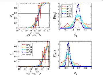
The sampling-based reconstruction algorithm we have proposed in the present paper rests upon the homogeneity assumption, according to which any subset of nodes picked at random provides a representative value of the density of the whole network. Table 2 collects the estimations of the link density, averaged over all sampled subsets of a given cardinality: remarkably, the obtained values are accurate even for low cardinalities. In order to assess the magnitude of fluctuations, we have also explicitly computed the empir-ical probability distributions of the link density estimates, obtained by random sampling our nodes subsets. These distributions are shown in Fig. 1 (right panels). Naturally, the smaller the cardinality of the considered nodes subsets, the more spaced the values of the observable link density and the less smooth the corresponding probability distribution. These findings suggests that our homogeneity assumption is indeed verified, provided that nodes are sampled according to the random selection scheme (Genois et al. 2015).

(9)

(10)

Fig. 1Left panels: scatter plots of the link densitycIversus the internal total strengthstotI of the subsetI.

Nodes characterized by large values of the total strength tend to form densely-connected groups, while nodes characterized by small values of the total strength tend, on the contrary, to form loosely-connected groups.Right panels: empirical probability distributions of the link densitycI, when nodes belonging toIare

chosen randomly. Each distribution is peaked around the density value of the whole network.Toppanels refer to the WTW,bottompanels to e-MID

severely overestimate the overall network density), nor towards the “periphery” portion of nodes (which would lead to severely underestimate the overall network density). Inter-estingly, in a recent paper comparing several network sampling techniques was found that the least biased sampling scheme for estimating a given network density is precisely the random-nodes one (Blagus et al. 2016).

Conclusions

The present contribution proposes a recipe to reconstruct a network from a very lim-ited amount of information. In particular, we address the problem of inferring the binary and the weighted structure of a given network from the knowledge of the nodes strengths and the link density of only a subset of nodes. As we have shown in the paper, the best sampling scheme is the random-nodes selection scheme which ensures that an accurate estimation of the whole network density can indeed be achieved. On the contrary, select-ing nodes on the basis of more informative structural properties (as the degree, or the strength) could bias the estimation of the connectance towards unrealistically too large, or too small, values. The role played by the available piece of topological information is fundamental not only to achieve an accurate reconstruction of the purely binary structure but also of the weighted structure, as evident upon inspecting Table 1.

(11)

different random subsets (even with different cardinality) are characterized by very sim-ilar densities, in turn implying that the whole network density can be estimated (with a high degree of accuracy) by considering a subset randomly drawn from the whole set of nodes. However, the proposed algorithm can be also used to reconstruct networks with a modular structure, upon tuning the link densities of the different modules via Eq. (4): examples are provided by interbank networks structured into jurisdictions, the latter playing the role of the subsets to be reconstructed.

Appendix 1

A pseudo-code summarizing the main steps of the reconstruction algorithm presented in the paper follows.

Algorithm 1:Network reconstruction via density sampling

Input: in- and out-strengths{sin_i }N_i₌₁,{sout_i }N_i₌₁and link density of a subsetI,

cI = _n_I_(nL_II₋₁₎.

begin

solve the equationcI= cIin order to determinez:

cI=

1

nI(nI−1)

i∈I

j(=i)∈I

zsout_i sin_j

1+zsout_i sin_j ;

definepij= zs

out i sinj

1+zsout i sinj

;

form=1. . .Mdo fori<jdo

calculate the correction to the gravity-like estimation

W

sout_j sin_j

l(=j)soutl sinl

⎡ ⎢

⎣ 1

k(=i) s

out k s

in k

m(=k)soutm sinm ⎤ ⎥ ⎦;

connectiandjwith a weight drawn from the following Bernoulli distribution

wij=

⎧ ⎨ ⎩

0, 1−pij,

sout i sinj

W +w

(3) ij

1 pij, pij.

end end

verify the goodness of the achieved reconstruction by calculating the ensemble average of indicators likeTPR,SPC,PPV,ACCandθ;

end

(12)

Appendix 2

Additional years have been analysed for both the WTW and e-MID (see Tables 3 and 4).

Table 3Statistical indicators used to evaluate the performance of our sampled-based reconstruction

method, for different cardinalitiesnof the known subsetI. Results are shown together with the 95%

confidence intervals (not shown whenever their difference affects the significant digits beyond the third one)

WTW n=5(CI 95%) n=10(CI 95%) n=20(CI 95%) n=50(CI 95%)

1950 - Link density (true: 0.402) 0.401 [0.375;0.426] 0.402 [0.387;0.416] 0.401 [0.393;0.409] 0.400 [0.396;0.403] 1950 - Accuracy 0.736 [0.731;0.741] 0.747 [0.746;0.749] 0.751 0.752

1950 - Cosine similarity 0.460 [0.458;0.462] 0.463 0.463 0.463

1960 - Link density (true: 0.383) 0.329 [0.305;0.352] 0.343 [0.330;0.357] 0.346 [0.338;0.355] 0.348 [0.344;0.353] 1960 - Accuracy 0.737 [0.734;0.741] 0.746 0.749 [0.748;0.750] 0.751

1960 - Cosine similarity 0.586 0.591 0.591 0.591

1980 - Link density (true: 0.468) 0.484 [0.458;0.510] 0.470 [0.455;0.485] 0.471 [0.461;0.481] 0.463 [0.458;0.469] 1980 - Accuracy 0.719 [0.715;0.723] 0.731 [0.730;0.733] 0.734 [0.733;0.735] 0.736

The considered cardinalitiesn=5, 10, 20, 50 correspond to percentages ranging from2% to25% of the total number of nodes. The true link densities calculated on the entire networks for the various periods are shown in brackets for reference

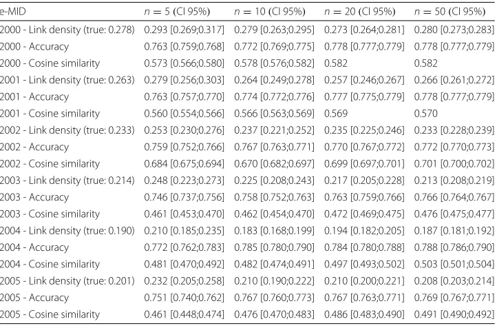
Table 4Statistical indicators used to evaluate the performance of our sampled-based reconstruction

method, for different cardinalitiesnof the known subsetI. Results are shown together with the 95%

confidence intervals (not shown whenever their difference affects the significant digits beyond the third one)

e-MID n₌5₍CI 95%₎ n₌10₍CI 95%₎ n₌20₍CI 95%₎ n₌50₍CI 95%₎

2000 - Link density (true: 0.278) 0.293 [0.269;0.317] 0.279 [0.263;0.295] 0.273 [0.264;0.281] 0.280 [0.273;0.283]

2000 - Accuracy 0.763 [0.759;0.768] 0.772 [0.769;0.775] 0.778 [0.777;0.779] 0.778 [0.777;0.779] 2000 - Cosine similarity 0.573 [0.566;0.580] 0.578 [0.576;0.582] 0.582 0.582

2001 - Link density (true: 0.263) 0.279 [0.256;0.303] 0.264 [0.249;0.278] 0.257 [0.246;0.267] 0.266 [0.261;0.272] 2001 - Accuracy 0.763 [0.757;0.770] 0.774 [0.772;0.776] 0.777 [0.775;0.779] 0.778 [0.777;0.779]

2001 - Cosine similarity 0.560 [0.554;0.566] 0.566 [0.563;0.569] 0.569 0.570

2002 - Link density (true: 0.233) 0.253 [0.230;0.276] 0.237 [0.221;0.252] 0.235 [0.225;0.246] 0.233 [0.228;0.239] 2002 - Accuracy 0.759 [0.752;0.766] 0.767 [0.763;0.771] 0.770 [0.767;0.772] 0.772 [0.770;0.773] 2002 - Cosine similarity 0.684 [0.675;0.694] 0.670 [0.682;0.697] 0.699 [0.697;0.701] 0.701 [0.700;0.702] 2003 - Link density (true: 0.214) 0.248 [0.223;0.273] 0.225 [0.208;0.243] 0.217 [0.205;0.228] 0.213 [0.208;0.219]

2003 - Accuracy 0.746 [0.737;0.756] 0.758 [0.752;0.763] 0.763 [0.759;0.766] 0.766 [0.764;0.767] 2003 - Cosine similarity 0.461 [0.453;0.470] 0.462 [0.454;0.470] 0.472 [0.469;0.475] 0.476 [0.475;0.477] 2004 - Link density (true: 0.190) 0.210 [0.185;0.235] 0.183 [0.168;0.199] 0.194 [0.182;0.205] 0.187 [0.181;0.192] 2004 - Accuracy 0.772 [0.762;0.783] 0.785 [0.780;0.790] 0.784 [0.780;0.788] 0.788 [0.786;0.790]

2004 - Cosine similarity 0.481 [0.470;0.492] 0.482 [0.474;0.491] 0.497 [0.493;0.502] 0.503 [0.501;0.504] 2005 - Link density (true: 0.201) 0.232 [0.205;0.258] 0.210 [0.190;0.222] 0.210 [0.200;0.221] 0.208 [0.203;0.214] 2005 - Accuracy 0.751 [0.740;0.762] 0.767 [0.760;0.773] 0.767 [0.763;0.771] 0.769 [0.767;0.771] 2005 - Cosine similarity 0.461 [0.448;0.474] 0.476 [0.470;0.483] 0.486 [0.483;0.490] 0.491 [0.490;0.492]

(13)

Acknowledgments

This work was supported by the EU projects CoeGSS (grant num. 676547), Multiplex (grant num. 317532), Shakermaker (grant num. 687941), SoBigData (grant num. 654024), GrowthCom (grant num. 611272) and the FET projects SIMPOL (grant num. 610704) and DOLFINS (grant num. 640772). AG acknowledges the CNR Strategic Project CRISISLAB funded by Italian Government. DG acknowledges support from the Econophysics foundation (Stichting Econophysics, Leiden, the Netherlands).

Authors’ contributions

TS, GC, AG and DG participated in the design of the analysis. TS and GC performed the statistical analysis. All authors wrote, read and approved the final manuscript.

Competing interests

The authors declare that they have no competing interests.

Author details

1_{IMT School for Advanced Studies Lucca, Piazza S.Francesco 19, 55100 Lucca, Italy.}2_{Istituto dei Sistemi Complessi (ISC)}

-CNR, UoS Sapienza, Dipartimento di Fisica, Universitá “Sapienza”, Piazzale Aldo Moro 5, 00185 Rome, Italy.

3_{Instituut-Lorentz for Theoretical Physics, Leiden Institute of Physics, University of Leiden, Niels Bohrweg 2, 2333 CA}

Leiden, The Netherlands.

Received: 20 October 2016 Accepted: 11 January 2017

References

Anand K, Craig B, von Peter G (2014) Filling in the blanks: Network structure and interbank contagion. Quant Finance 15:625–636

Baral P, Fique JP (2012) Estimation of bilateral exposures - a copula approach. Mimeo. http://www.cirano.qc.ca/ conferences/public/pdf/networks2012/02-BARAL-FIQUE-Estimation_of_Bilateral_Exposures-A_Copula_Approach. pdf

Bishop YM, Fienberg SE, Holland PW (2007) Discrete Multivariate Analysis: Theory and Practice. Springer-Verlag, New York Blagus N, Subelj L, Bajec M (2016) Empirical comparison of network sampling techniques. arxiv:1506.02449. https://arxiv.

org/pdf/1506.02449v2.pdf

Cimini G, Squartini T, Gabrielli A, Garlaschelli D (2015a) Estimating topological properties of weighted networks from limited information. Phys Rev E 92:040802. doi:10.1103/PhysRevE.92.040802

Cimini G, Squartini T, Garlaschelli D, Gabrielli A (2015b) Systemic risk analysis on reconstructed economic and financial networks. Sci Rep 5:15758. doi:10.1038/srep15758

De Masi G, Iori G, Caldarelli G (2006) Fitness model for the italian interbank money market. Phys Rev E 74:066112. doi:10.1103/PhysRevE.74.066112

Drehmann M, Tarashev N (2013) Measuring the systemic importance of interconnected banks. J Financ Intermediation 22(4):586–607. doi:10.1016/j.jfi.2013.08.001

Fagiolo G, Reyes J, Schiavo S (2010) The evolution of the world trade web: a weighted-network analysis. J Evol Econ 20(4):479–514. doi:10.1007/s00191-009-0160-x

Genois M, Vestergaard C, Cattuto C, Barrat A (2015) Compensating for population sampling in simulations of epidemic spread on temporal contact networks. Nat Commun 6(8860)

Gleditsch KS (2002) Expanded trade and gdp data. J Confl Resol 46(5):712–724

Hałaj G, Kok C (2013) Assessing interbank contagion using simulated networks. Comput Manag Sci 10(2):157–186. doi:10.1007/s10287-013-0168-4

Iori G, Jafarey S, Padilla FG (2006) Systemic risk on the interbank market. J Econ Behav Organ 61(4):525–542. doi:10.1016/j.jebo.2004.07.018

Mastrandrea R, Squartini T, Fagiolo G, Garlaschelli D (2014) Enhanced reconstruction of weighted networks from strengths and degrees. New J Phys 16(4):043022

Mastromatteo I, Zarinelli E, Marsili M (2012) Reconstruction of financial networks for robust estimation of systemic risk. J Stat Mech Theory Exp 03:03011. doi:10.1088/1742-5468/2012/03/P03011

Montagna M, Lux T (2014) Contagion risk in the interbank market: A probabilistic approach to cope with incomplete structural information. Kiel working papers, Kiel Institute for the World Economy. https://www.ifw-members.ifw-kiel. de/publications/1937-contagion-risk-in-the-interbank-market-a-probabilistic-approach-to-cope-with-incomplete-structural-information/1937_KWP.pdf

Musmeci N, Battiston S, Caldarelli G, Puliga M, Gabrielli A (2013) Bootstrapping topological properties and systemic risk of complex networks using the fitness model. J Stat Phys 151(3):720–734. doi:10.1007/s10955-013-0720-1

Peltonen TA, Rancan M, Sarlin P (2015) Interconnectedness of the banking sector as a vulnerability to crises. Working Paper 1866, ECB European Central Bank. http://www.ecb.europa.eu/pub/pdf/scpwps/ecbwp1866.en.pdf Squartini T, Caldarelli G, Cimini G (2016) Stock markets reconstruction via entropy maximization driven by fitness and

density. arXiv:1606.07684. https://arxiv.org/pdf/1606.07684v1.pdf

Upper C (2011) Simulation methods to assess the danger of contagion in interbank markets. J Financ Stability 7(3):111–125. doi:10.1016/j.jfs.2010.12.001