Thought Chart: tracking the thought with manifold learning during emotion regulation

ORIGINAL RESEARCH

Thought Chart

: tracking the thought

with manifold learning during emotion

regulation

Mengqi Xing

_{, Johnson GadElkarim}

_{, Olusola Ajilore}

_{, Ouri Wolfson}

_{, Angus Forbes}

_{, K. Luan Phan}

_,

Heide Klumpp

_{and Alex Leow}

Abstract

The Nash embedding theorem demonstrates that any compact manifold can be isometrically embedded in a Euclidean space. Assuming the complex brain states form a high-dimensional manifold in a topological space, we propose a manifold learning framework, termed Thought Chart, to reconstruct and visualize the manifold in a low-dimensional space. Furthermore, it serves as a data-driven approach to discover the underlying dynamics when the brain is engaged in a series of emotion and cognitive regulation tasks. EEG-based temporal dynamic functional connectomes are created based on 20 psychiatrically healthy participants’ EEG recordings during resting state and an emotion regulation task. Graph dissimilarity space embedding was applied to all the dynamic EEG connectomes. In order to visualize the learned manifold in a lower dimensional space, local neighborhood information is reconstructed via k-nearest neighbor-based nonlinear dimensionality reduction (NDR) and epsilon distance-based NDR. We showed that two neighborhood constructing approaches of NDR embed the manifold in a two-dimensional space, which we named Thought Chart. In Thought Chart, different task conditions represent distinct trajectories. Properties such as the distribution or average length in the 2-D space may serve as useful parameters to explore the underlying cognitive load and emotion processing during the complex task. In sum, this framework is a novel data-driven approach to the learning and visualization of underlying neurophysiological dynamics of complex functional brain data.

Keywords: Thought Chart, Nonlinear dimensionality reduction, Nearest neighbor, Manifold learning, EEG connectome, Emotion regulation

© The Author(s) 2018. This article is distributed under the terms of the Creative Commons Attribution 4.0 International License (http://creat iveco mmons .org/licen ses/by/4.0/), which permits unrestricted use, distribution, and reproduction in any medium, provided you give appropriate credit to the original author(s) and the source, provide a link to the Creative Commons license, and indicate if changes were made.

1 Background

The Nash embedding theorems [1, 2] showed that any Riemannian n-manifold with a C1 positive metric has an isometric embedding in a Euclidean space of dimension 2n+1, even in any small portion of this space. Since the Gaussian curvature of a surface is invariant under local isometry based on the Theorema Egregium [3], the mani-fold properties in a low-dimensional space can provide an insight into the topological structure of the brain. Recent advent in structural and functional neuroimag-ing has further suggested that brain imagneuroimag-ing data may

construct a smooth and differentiable manifold, in which local neighborhood properties can assist in recognizing the underlying pattern in trajectories of brain develop-ment [4], discriminating different types of brain tumors [5], and improving the imaging registration accuracy [6]. However, the manifold associated with temporally varying brain dynamics imaging data has not yet been explored. Here, we propose a framework to examine the intrinsic geometry of the mind’s topological space of functional brain imaging via dissimilarity-based manifold learning.

We assume brain states compose a high-dimensional space [4, 7], which can be reconstructed and visualized in a low-dimensional space via dimensionality reduc-tion. Common dimensionality reduction approaches including principal component analysis (PCA) and linear

Open Access

*Correspondence: [email protected]

4 _{Department of Psychiatry, Department of Bioengineering, University}

of Illinois at Chicago, Chicago, IL, USA

discriminant analysis (LDA) are often used in functional brain networks to visualize select regions of interest [8,

9]. However, a linear approach cannot recognize nonlin-ear structures in a high-dimensional space [9], making it unsuitable for preserving the global intrinsic geometry for complex dynamic brain data. Nonlinear dimensional-ity reduction approach isomap yields global coordinates which provide a simple way to analyze and manipulate high-dimensional observations in terms of their intrin-sic nonlinear degrees of freedom and produce a globally optimal low-dimensional Euclidean representation [10].

The functional network data are informed by electro-encephalogram (EEG) for its high temporal resolution, coupled with the emotion regulation task. The synchro-nization of response systems is highly dynamic when human brains are engaging in emotion and cognitive tasks [11]. Thus, with proper sectioning, the synchronic-ity between regions of a brain network can be described, in the form of a connectome, using a phase-based con-nectivity analyses approach, weighted phase lag index (WPLI) [12]. Guided by our own published research results, theta wave may be the most sensitive among all EEG frequencies in investigating EEG networks in emo-tion regulaemo-tion task (ERT) [13, 14]. Therefore, we selected theta wave network connectivity as the input for our manifold learning.

Here, we propose a manifold learning framework, Thought Chart, to explore the underlying intrinsic geom-etry of dynamic functional networks. The hypothesis of this manifold learning is that the reconstructed manifold will reflect different properties of the brain’s state during tasks. Additionally, by sampling the space, we can extract specific aspects of the trajectory in this manifold that reflect task performance, such as coordinates and their distribution and levels of scattering [15]. To recover the local neighborhood information needed for the nonlin-ear dimensionality reduction (NDR) step, here we tested two strategies in searching for local neighbors: K-near-est neighbor (KNN), which sets each point to search for its k-nearest points; and epsilon radius, which sets each point to search for all points within a fixed radius ε . Properties of Thought Chart constructed by these two approaches will be evaluated to see how neighborhood identification influences the intrinsic geometry of human brain.

2 Methods

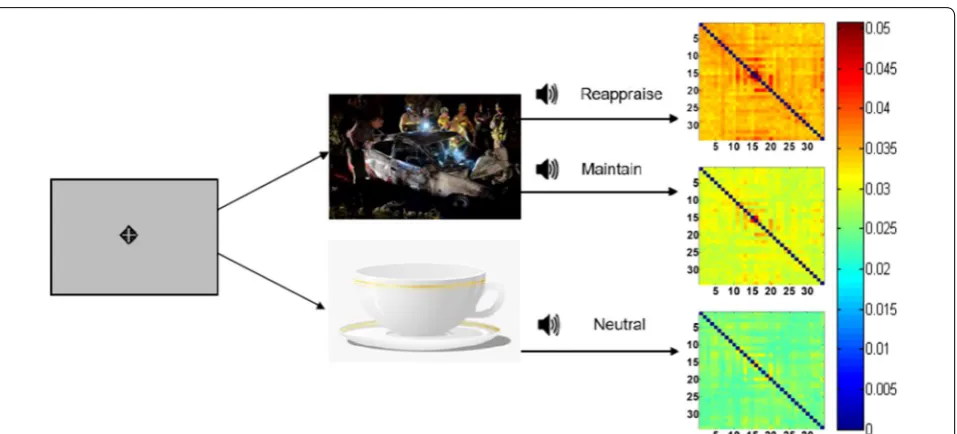
2.1 Data acquisition and emotion regulation tasks (ERT) EEG data were collected from 20 psychiatrically healthy participants (age: 27.2±9.3 ) using the Biosemi system (Biosemi, Amsterdam, the Netherlands) with an elastic cap with 34 scalp channels. Each participant underwent one session of ERT (Fig. 1). During ERT, participants

were requested to look at pictures displayed on the screen and listen to a corresponding auditory guide. Two types of pictures will be on display for 7  s in random orders: emotionally neutral pictures (landscape, everyday objects, etc.) and negative pictures (car crash, nature dis-asters, etc.). An auditory guide will come after the picture on display for 1 s, instructing the participant to “Look”: viewing the neutral pictures; to “Maintain: viewing the negative pictures as they normally would; or to “Reap-praise”: viewing the negative pictures while attempting to reduce their negative emotion by reinterpreting the meaning of pictures [16, 17]. A separate session of eight-minute eyes-open EEG resting states was recorded for later manifold learning. All EEG data were preprocessed using Brain Vision Analyzer (Brain Products, Gilching, Germany), by first segmenting task trials into 7  s seg-ments. A sliding window in size of 0.5 s and a step size of 0.05 were applied to create the dynamic data. (The first and last five time points were discarded, resulting in 130 time points per session.) Frequencies of interest were set from 1Hz to 50Hz in increments of 1Hz. The final out-put of each subject was averaged over trials within the same task. Resting-state data were processed under the same parameter. Due to the non-trial-based setting of the recording, resting state will only serve as bases that further create contrast in manifold learning. Thus, the manifold properties associated with the resting-state connectomes in the Euclidean space are not included in our final analyses.

2.2 Weighted phase lag index‑based EEG connectome As functional communications between two brain regions result in synchronized or phase-coupled EEG readouts, in this study we used weighted phase lag index (WPLI) computed [12] between the times series of two channels to form EEG connectomes (each of which is a symmetric 34 by 34 matrix). Mathematically, WPLI is defined as:

where imag(Sxyt) indicate the cross-spectral

den-sity at time t in the complex plane xy, and sgn is the sign function (−1,+1or0) [12]. The connectivity

matrices were generated with the MATLAB toolbox Fieldtrip (Donders Centre for Cognitive Neuroimag-ing, Nijmegen, the Netherlands). The final output time-dependent EEG connectome for an individual task of each subject is arranged as 34×34×50×130

(channel×channel×frequency×time). In this study, (1) WPLI_xy= n

−1n t=1

imag(S_xyt)

sgn(imag(S_xyt)) n−1n

t=q

we primarily focused on the manifold informed by theta wave (4–7 Hz) in EEG connectomes.

2.3 Learning the manifold with graph dissimilarity space embedding

To collect sufficient amount of data points to learn the intrinsic geometry of a high-dimensional manifold, we utilized the EEG connectomes from all subjects at all time points as sampling possible states of the manifold that is shared among all subjects. Then, graph dissimilar-ity space embedding is used to represent each connec-tome as a point in a very high-dimensional space (over 104), which is described below [18, 19]. Assuming labeled sample graph set G=G1, ...,Gn has n ”prototype” graph observations Gi∈G (the set of all possible graphs under consideration) and d is the distance metric that can be computed between two graphs d:G×G→ [0,∞) , then any graph X∈G can be represented using ϕ_nG:G→R_n, defined as the n-dimensional vector

ϕ_nG(X)= [d(X,G1), ...d(X,Gn)] . In this way, any graph

set can be represented by a set of real numbers. In our case, all the connectomes were initially used as proto-types for an unsupervised learning. Thus, the number of dimensions is in the same order as the number of obser-vations in the dataset.

Reconstructing the local neighborhood reconstruction. Here, we emphasize that this step is crucial in order to properly learn the manifold’s intrinsic geometry, as d (which is used to define coordinates in the embedding space, and thus not intrinsic to the manifold) will not properly inform geodesics (the shortest paths on the manifold, which is an intrinsic property) except in local neighborhoods. While such a construction calls for a “good” choice of the distance function d, we posit that given a sufficiently large amount of data points the learned manifold will converge to the true manifold with any reasonably chosen d. Given two connectome matri-ces X and Y, a natural choice, which we adopted here, is the Euclidean distance: d(X,Y)=

ij(Xij−Yij)2 and

ϕ_nG(X)−ϕG_n(Y)=

k(d(Y,Gk)−d(X,Gk))2 .

2.4 Nonlinear dimensionality reduction

Once the local neighborhood is learned, a matrix rep-resenting this high-dimensional manifold was recon-structed into a lower dimensional Euclidean space via NDR. Once this is achieved, Thought Chart of any given individual can be constructed by tracing the trajectory of the time-dependent connectome of that subject for any given task. In this case, we selected isomap, a non-linear prototypical isometric embedding procedure which entails the computation of geodesics based on

neighborhood information followed by the (quasi-)iso-metric embedding of the geodesics.

To provide a good approximation to geodesic distance, the first step of isomap is to determine the neighbors of each point on the low-dimensional manifold based on the distance matrix acquired from the previous step [20]. Here, we compared two common approaches to determine whether two points are neighbors: the k-iso-map method and the ε−isomap method. K-isomap utilized the k-nearest neighbor algorithm to determine neighbors, while ε-isomap includes all the points within

some fixed radius ε . The relationships of the

neighbor-hood are represented in a weighted graph D in which D(X,Y)=d(X,Y) if X and Y are neighbors,

other-wised(X,Y)= ∞ [20]. The second step relies on

apply-ing the classic multidimensional scaling (MDS) to the centered squared geodesic distance matrix, whose eigen-decomposition provides the basis for lower dimensional embedding.

2.5 Exploration of ERT Thought Chart

The resting state and the emotion regulation will be visu-alized in a two-dimensional Euclidean space. To quantify the dynamic properties and thought trajectory of emo-tion regulaemo-tion, we summarize the Euclidean distance along the trajectory in this 2-D space (average length) and the average distance from the centroid (spreadness) for each subject. For each subject with time length t ∈ [1, 130] , the average trajectory length is described as:

where x, y are the position of each point in the 2-D space. And the spreadness is described as:

3 Results

3.1 Thought Chart construction

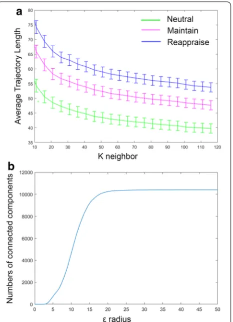
After averaging across theta frequencies (4–7 Hz) and combining both resting and ERT theta connectomes for all time points, 20 healthy subjects thus contributed a total of 10400 connectomes ( 130×20×4 ). We repeated our analyses with a range of k and ε values. In k-isomap,

the trajectory length difference across three conditions is stable with k ranging from 10 to 120. Though we pre-sented results with k=30(0.3% of the total points), the reported differences in tasks are consistent with any k in this range (Fig. 8a). In the case of ε-isomap, a point

can potentially be excluded after the neighborhood (2)

L=

t=1

(xt−xt+1)2+(yt−yt+1)2/(130−1)

(3) S=

t=130

t=1

construction step if it has no neighbors within an ε radius

(unlike in k-isomap, all nodes are retained after neighbor-hood construction). Therefore, the number of connected components is the main factor in selecting the ε . When ε

is larger than 28, the size of connected components con-verges to a constant, where 10,371 out of 10,400 points are connected (Fig. 8b). As the number of dimensions reduced from 10,400 to 2, the reconstructed theta EEG manifold exhibited a principal dimension that is shared by all four states in both isomaps (x-axis in Figs. 2, 3) with a secondary up–down motion from one side to the other. Visually, this manifold thus resembles the shape of a snake by spiraling around its main axis. Moreover, the distribution along the first dimension follows an ordered transition: (from low to high amplitude) rest-ing (red), Neutral (green), Maintain (purple) and Reap-praise (blue), corresponding to increasing cognitive load of the tasks. The similar task distribution was observed with locally linear embedding (LLE) [21] (Fig. 2), a non-isometric NDR approach. Additionally, the embedding generated using simple PCA (a linear technique) does not recover the full nonlinear distribution seen in either iso-map or LLE.

3.2 K‑isomap

To further understand theta EEG connectome dynam-ics, we additionally studied the four distinct subregions of the manifold (i.e., segments of the “snake”): the head (primarily resting), the mid body (primarily Neutral), the posterior body (a mixture of Neutral, Maintain, and

Reappraise) and the tail (primarily Maintain and Reap-praise; Fig. 4). Sampling these segments reveals marked connectome differences. Analysis of the top ten edge strengths in the head region (Fig.  4a) demonstrated increased theta coupling in fronto-parieto-occipital leads while the body (Neutral-predominant, Fig. 4b; Maintain/Reappraise dominant, Fig. 4c) is characterized by predominant theta coupling between occipital leads. Last, the tail (Maintain/Reappraise only, Fig. 4d) revealed increased theta coupling between frontal and parietal leads.

3.3 ε‑isomap

Thought Chart of the ε-isomap presents a similar

distri-bution along the principle dimension. Taking samples for the head, mid body, posterior body, and tail, the over-all connectivity of the average connectome is increas-ing monotonically, which is different from k-isomap. The top ten edge strengths in the head region (Fig. 5a) demonstrated strong parieto-central and occipital theta coupling, while the body (Fig. 5b, c) presented increas-ing theta couplincreas-ing within occipital channels. Lastly, the increased theta coupling between frontal and occipital leads can be observed at the tail (Fig. 5d).

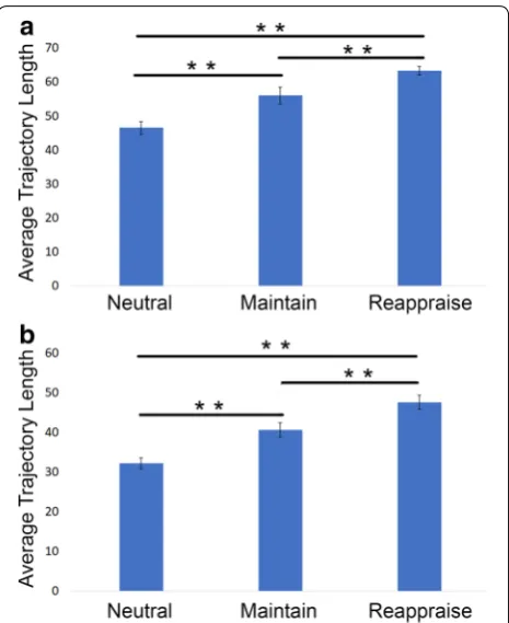
3.4 Average trajectory length and spreadness

In k-isomap Thought Chart, average trajectory length in the Euclidean space was significantly longer in more complex tasks (Fig.  6a), (one-way ANOVA:

Fig. 2 An example Thought Chart during Reappraise learned from the temporal EEG connectomes of 20 healthy subjects, both at rest and during ERT, using NDR methods of isomap (left) and LLE (lower right), as well as standard PCA (upper right). Visually, NDR methods yielded an ordered transition from resting, Neutral, Maintain to Reappraise along the manifold’s principal dimension (isomap dimension 1)

Fig. 3 An example Thought Chart using NDR method of ε-isomap, Thought Chart follows the same ordered transition of resting, Neutral, Maintain to

Fig. 4 Mean 34×34 _{theta EEG connectomes of four distinct segments: the head (a), the mid and posterior body (b, c) and the tail (d) (left). For} each mean connectome, its ten strongest edges were visualized on the layout of the electrodes (right)

vs. Maintain: p=0.008 , Maintain vs. Reappraise: p=0.004 , Neutral vs. Reappraise p<0.001 ). In ε -isomap Thought Chart, a similar trend is observed, where subjects tend to “travel” longer distance in Thought Chart during tasks with higher cog-nitive demand (Fig.  6b). (One-way ANOVA:

df =2,F =21.75,p<0.001 , paired t test: Neutral

vs. Maintain: p=0.002 , Maintain vs. Reappraise: p=0.003 , Neutral vs. Reappraise p<0.001 .)

Fur-thermore, task differences not only were reflected in the average distance traveled, but also observed in the level of scattering measured using spread-ness (Fig. 7), in both k-isomap (one-way ANOVA:

df =2,F=15.61p<0.001, paired t test: Neutral vs. Maintain: p=0.015 , Maintain vs. Reappraise: p=0.047 , Neutral vs. Reappraise p<0.001 ) and ε

-iso-map (one-way ANOVA: df =2,F =19.20,p<0.001 , paired t test: Neutral vs. Maintain: p=0.008 ,

Main-tain vs. Reappraise: p=0.017 , Neutral vs. Reappraise

p<0.001.)

4 Discussion

In this study, we proposed a novel unsupervised mani-fold learning framework to construct a state space, in the form of a manifold embedded in 2-D that quasi-isometri-cally visualizes EEG connectome dynamics. Moreover, in this space one can visualize time-dependent brain activi-ties as a trajectory or Thought Chart. Using the temporal dynamic EEG connectome, two neighborhood construc-tion algorithms are applied to visualize the state space in 2-D. Both k-isomap and ε-isomap are able to compose a

highly dynamic and complex geometry, where distinct subregions are distributed along the principle dimen-sion (x-axis in the 2-D space). The baseline resting state is concentrated on one end, followed by mostly Neutral points that can be observed later along the x-axis, while Maintain and Reappraise are mixed, from the poste-rior section on to the end. Note that this transition cor-responds to different mental states, suggesting that the manifold has a principal dimension that is primarily lin-ear, and a vertical motion around this principal dimen-sion whose amplitude increases with cognitive demands. In this context, this manifold may resemble dynamical systems on a torus [22] (the surface of a doughnut), in that trajectories are generated by the product of distribu-tion along the principal dimension and a minor up–down motion in the second dimension.

By sectioning the region where different tasks concen-trated, matrices can be defined to represent these regions. As similar Thought Chart trajectories are, regional matri-ces of k-isomap and ε-isomap however can be different.

There are few possible explanations. First, even if each region appears to have a similar composition of tasks, due to the different neighborhood constructing strat-egy, the points being included in the same regions are not necessarily the same. Second, the sectioning of the head, body, and tail is arbitrary; hence, it can only pro-vide an approximate matrix representation without rig-orously controlling the number of points of this region. However, the strongest theta couplings in each region are similar between two methods. Based on the strongest coupling, the manifold comprises subspaces represent-ing restrepresent-ing, visual processrepresent-ing (a common feature of Neu-tral, Maintain, and Reappraise), and cognitive control (a distinct feature of Reappraise). Edge strength analyses of the manifold-sampled EEG connectomes demonstrated increased patterns of theta coupling that are highly con-sistent with previous reports of frequency-band coupling associated with the resting state [23], visual processing [24], and cognitive control [25].

As it is shown in Figs. 2 and 3, Thought Chart is able to visualize an individual’s “mind travels” in a two-dimen-sional space in this 7-s session. It thus allows us to quan-tify the temporal dynamics of EEG brain networks by

looking into properties such as the distribution and tra-jectory length. For healthy participants, the mind is more or less “static” when the task is simple and becomes more dynamic as the task requires higher cognitive demand. These properties can be extracted as biomarkers for mind state predictions in future applications.

Limitations of our approach merit further discussion. First, the parameter setting for ε-isomap can be very sen-sitive since ε is defined as a distance which can be tuned to go either fine (local) or coarse (global) (Fig. 8b). In this dataset, the reconstructed trajectory is stable as the ε changed within a certain range. However, in future appli-cations, it may create further complexity in determining the optimal ε , especially if the data are sensitive toward ε . Secondly, it may be inappropriate to compare these thought chart metrics in the resting state with those from Neutral, Maintain, and Reappraise. This is due to the nature of a task-free design (resting state) versus a task-related design during ERT. Unlike in the resting state when research participants were simply instructed

to do nothing (and thus leading to mind wandering), in ERT there is a clear “begin” and “end” cue for all Neu-tral, Maintain, and Reappraise sessions and participants were instructed to accomplish a certain task between the cues. Thus, we are able to precisely calculate trajectories by averaging across trials and compare them across three task conditions. However, the resting-state data were col-lected from a continuous session, during which partici-pants were not instructed to think in any particular way. Therefore, the resting-state data were only included as “baseline reference” in dissimilarity embedding and in isomap visualization but not during subsequent quanti-tative analyses. Moreover, as a quasi-isometric technique isomap aims to preserve the pairwise geodesics on the manifold, i.e., approximating global isometry when the embedding is constrained to a given dimension. By con-trast, other classes of local NDR methods such as LLE unfold the manifold by preserving local linear recon-struction relationship (i.e., local parameterization) of each point within its neighborhood. Furthermore, as the Theorema Egregium only guaranteed the invariance of

Fig. 7 Spreadness of each condition in 2-D isomap spaces, both k-nearest neighbor approach (a) and the epsilon-based approach (b). In k-isomap, the spreadness in Neutral: 65.61±2.74 , Maintain: 79.51±3.64 , Reappraise: 88.67±2.27 ; in ε-isomap, the spreadness in

Neutral: 45.43±2.09 , Maintain: 55.78±2.27 , Reappraise: 64.30±2.09 .

Both suggest the Thought Chart is more scattered as the task condition becomes more complex. Significant findings in group t test are indicated with **p<0.01 _and *p<0.05

Gauss curvature for complete isometric embeddings of two manifolds, it is unclear whether the manifold con-structed using one NDR technique is necessarily more “correct.” Nevertheless, both LLE and isomap recover a principal dimension and a up–down motion around it, while simple linear techniques such as PCA did not. We thus posit that the highly structured complex geometry recovered using our framework may indeed inform the hidden properties of brain dynamics and the underlying neurophysiological mechanisms that generate them. Authors’ contributions

MX processed the EEG data and completed the network estimation. EEG data were collected under the administration of HK. AL, OA, and OW constructed the dissimilarity embedding and non-dimensionality reduction framework. MX and JG wrote the complete Thought Chart scripts in Matlab. MX, JG, OA, AL, AF, HK, and KLP drafted and revised the manuscript together. All authors read and approved the final manuscript.

Author details

1 _{Department of Bioengineering, University of Illinois at Chicago, Chicago,}

IL, USA. 2 _{Department of Computer Science, University of Illinois at Chicago,}

Chicago, IL, USA. 3 _{Department of Psychiatry, University of Illinois at Chicago,}

Chicago, IL, USA. 4 _{Department of Psychiatry, Department of Bioengineering,}

University of Illinois at Chicago, Chicago, IL, USA.

Acknowlegdements

This work was supported by NIMH K23MH093679 (HK) and in part by NIMH R01MH101497 (KLP) and the Center for Clinical and Translational Research (CCTS) UL1RR029879, and University of Illinois at Chicago Campus Research Board Award.

Competing interests

The authors declare that they have no competing interests.

Ethics approval and consent to participate

All procedures performed in studies involving human participants were in accordance with the ethical standards of the institutional and/or national research committee and with the 1964 Helsinki declaration and its later amendments or comparable ethical standards.

Consent for publication

Informed consent was obtained from all individual participants included in the study.

Publisher’s Note

Springer Nature remains neutral with regard to jurisdictional claims in pub-lished maps and institutional affiliations.

Received: 10 February 2017 Accepted: 12 July 2018

References

1. Nash J (1954) C1 isometric imbeddings. Ann Math 60:383–396 2. Nash J (1956) The imbedding problem for Riemannian manifolds. Ann

Math 63:20–63

3. Gauss CF (1902) General investigations of curved surfaces of 1827 and 1825. Princeton University Library, Princeton

4. Aljabar P, Wolz R, Srinivasan L, Counsell SJ, Rutherford MA, Edwards AD, Hajnal JV, Rueckert D (2011) A combined manifold learning analysis of shape and appearance to characterize neonatal brain development. IEEE Trans Med Imaging 30:2072–2086

5. Cruz-Barbosa R, Vellido A (2011) Semi-supervised analysis of human brain tumors from partially labeled MRS information, using manifold learning models. Int J Neural Syst 21:17–29

6. Ye DH, Hamm J, Kwon D, Davatzikos C, Pohl, KM (2012) Regional manifold learning for deformable registration of brain MR images. In: Medical image computing and computer-assisted intervention − _{MICCAI 2012:} 15th international conference, Nice, France, October 1–5, 2012, proceed-ings, part III, pp 131–138. Springer, Berlin

7. Poldrack RA, Halchenko YO, Hanson SJ (2009) Decoding the large-scale structure of brain function by classifying mental states across individuals. Psychol Sci 20:1364–1372

8. Zhou Z, Chen Y, Ding M, Wright P, Lu Z, Liu Y (2009) Analyzing brain networks with PCA and conditional Granger causality. Hum Brain Mapp 30:2197–2206

9. Lotte F, Congedo M, Lécuyer A, Lamarche F, Arnaldi B (2007) A review of classification algorithms for EEG-based brain-computer interfaces. J Neural Eng 4:R1

10. Tenenbaum JB, Silva VD, Langford JC (2000) A global geometric frame-work for nonlinear dimensionality reduction. Science 290:2319–2323 11. Scherer KR (2009) The dynamic architecture of emotion: Evidence for the

component process model. Cognit Emot 23:1307–1351

12. Cohen MX (2013) Analyzing neural time series data: theory and practice. The MIT Press, London

13. Xing M, Tadayonnejad R, MacNamara A, Ajilore O, DiGangi J, Phan KL, Leow A, Klumpp H (2017) Resting-state theta band connectivity and graph analysis in generalized social anxiety disorder. NeuroImage: Clin 13:24–32

14. Xing M, Tadayonnejad R, MacNamara A, Ajilore O, Phan KL, Klumpp H, Leow A (2016) EEG based functional connectivity reflects cognitive load during emotion regulation. In: 2016 IEEE 13th international symposium on biomedical imaging (ISBI), pp. 771–774

15. Xing M, Ajilore O, Wolfson O, Abbott C, MacNamara A, Tadayonnejad R, Forbes A, Phan KL, Klumpp H, Leow A (2016) Thought chart: tracking dynamic EEG brain connectivity with unsupervised manifold learning. In: International conference on brain and health informatics, pp 149–157 16. Parvaz MA, MacNamara A, Goldstein RZ, Hajcak G (2012) Event-related induced frontal alpha as a marker of lateral prefrontal cortex activation during cognitive reappraisal. Cognit Affect Behavi Neurosci 12:730–740 17. Gross JJ (1998) The emerging field of emotion regulation: an integrative

review. Rev General Psychol 2:271–299

18. Bunke H, Riesen K (2008) Graph Classification Based on Dissimilarity Space Embedding. In: da Vitoria Lobo, N, Kasparis T, Roli F, Kwok JT, Geor-giopoulos M, Anagnostopoulos GC, Loog M (eds) Structural, syntactic, and statistical pattern recognition: joint IAPR international workshop, SSPR and SPR 2008, Orlando, USA, December 4–6, 2008. Proceedings, pp 996–1007. Springer, Berlin

19. Duin RPW, Loog M, Pekalska E, Tax DMJ (2010) Feature-based dissimilarity space classification. In: Unay D, Çataltepe Z, Aksoy S (eds) Recogniz-ing patterns in signals, speech, images and videos: ICPR 2010 contests, Istanbul, Turkey, August 23–26, 2010, contest reports. Springer, Berlin, pp 46–55

20. Yiming W, Kap Luk C, An extended Isomap algorithm for learning multi-class manifold. In: Proceedings of 2004 international conference on machine learning and cybernetics, vol 3426 (IEEE Cat. No.04EX826), pp 3429–3433

21. Roweis ST, Saul LK (2000) Nonlinear dimensionality reduction by locally linear embedding. Science 290:2323–2326

22. Tozzi A, Peters JF (2016) Towards a fourth spatial dimension of brain activ-ity. Cognit Neurodyn 10:189–199

23. Albrecht MA, Roberts G, Price G, Lee J, Iyyalol R, Martin-Iverson MT (2016) The effects of dexamphetamine on the resting-state electroencephalo-gram and functional connectivity. Hum Brain Mapp 37:570–588 24. Keil A, Costa V, Smith JC, Sabatinelli D, McGinnis EM, Bradley MM, Lang

PJ (2012) Tagging cortical networks in emotion: a topographical analysis. Human Brain Mapp 33:2920–2931