An alternative approach to the limits of predictability in human mobility

(1)

R E G U L A R A R T I C L E

Open Access

An alternative approach to the limits of

predictability in human mobility

Edin Lind Ikanovic and Anders Mollgaard

*

*_{Correspondence: [email protected]} Niels Bohr Institute, University of Copenhagen, Copenhagen, 2100, Denmark

Abstract

Next place prediction algorithms are invaluable tools, capable of increasing the efficiency of a wide variety of tasks, ranging from reducing the spreading of diseases to better resource management in areas such as urban planning. In this work we estimate upper and lower limits on the predictability of human mobility to help assess the performance of competing algorithms. We do this using GPS traces from 604 individuals participating in a multi year long experiment, The Copenhagen Networks study. Earlier works, focusing on the prediction of a participant’s whereabouts in the next time bin, have found very high upper limits (>90%). We show that these upper limits are highly dependent on the choice of a spatiotemporal scales and mostly reflect stationarity, i.e. the fact that people tend tonotmove during small changes in time. This leads us to propose an alternative approach, which aims to predict the next location, rather than the location in the next bin. Our approach is independent of the temporal scale and introduces a natural length scale. By removing the effects of stationarity we show that the predictability of the next location is significantly lower (71%) than the predictability of the location in the next bin.

Keywords: human mobility; predictability; limits

1 Introduction

The understanding of human mobility patterns has changed greatly in the last couple of decades. This has mainly been due to new technologies enabling human displacements to be studied with higher accuracy over a longer period of time. Starting with the tracking of bank notes [] as a proxy for human movement, studies quickly evolved towards the current use of hand held devices for tracking, using either GSM data [, ], connections to wifi hotspots [] or GPS receivers [] to determine location. The main results from these studies have been the discoveries of power laws governing step size and wait time dis-tributions [], a universal probability density governing human mobility [], and simple models capturing many statistical features of human mobility [–]. It has furthermore been explored how mobility is affected by recency [], exploration [], and return to pre-viously visited places [] and friends []. Such discoveries and models can help predict the spread of diseases [] and cellphone viruses [], and also enhance socio-economic forecasting [–], city planning [] and many other fields [, , ]. Further contribu-tion to progress in these areas can be made if geolocacontribu-tion data can be used to accurately predict an individual’s future whereabouts. A crucial part of this work is the construction

(2)

of viable evaluation mechanisms, thereby raising the question: what are the upper and lower limits,max_andmin_{, on the predictability of human mobility?}

This question was initially investigated using call detail records from , cellphones []. Each call corresponded to a known location represented by a Voronoi cell, around the closest cell tower, with an average area of  km_{. The known locations were grouped}

into  hour bins, giving a history of locationsTi, for each useri. The work focused on

determining how well the best possible algorithm can predict the location of an individual in the next time bin, givenTi. They reported an upper limit narrowly peaked atmax=

%and a lower limit ofmin= %.

This work led to questions being raised about possible biases introduced when using call detail records [] and about the inﬂuence of spatiotemporal scales []. The tempo-ral resolution [, ] and spatial resolution [, , ] were investigated with GSM and GPS data for smaller populations. Overall, it was found that the predictability increases with temporal resolution and decreases with spatial resolution. The limits of predictabil-ity, as deﬁned in [], therefore depend on the choice of temporal resolutiontand spatial resolutions.

Here we make the following conjecture:

(max,min)(t,s)→ whent→ ors→ ∞. ()

The rationale behind this expression is that the location of the next time bin will almost certainlynot change in both limits. At small time scales and at large spatial scales you always know where an individual is going to be in the next time bin: he/she will be in the same spatial bin. We therefore argue that the current limits on the predictability of mobility to a large extent reﬂect stationarity. Previous results therefore mix two diﬀerent questions, namely

– How long will an individual stay in his/her current location?

– Where will he/she go next?

Here we propose an analysis that is able to separate out the ﬁrst question such that we can concentrate on the second. This is achieved by focusing on thenext location, rather than the location in the next bin. This approach is independent oft, provided a small sampling rate. By introducing a natural length scale, we are able to get a single number for the predictability of human mobility, rather than a function of spatiotemporal resolution. Our new approach shows that the upper limit on the predictability of this type of mobility is around∼%, rather than the >%found in earlier works. We thereby show that the high upper limits of previous works mostly reﬂect stationarity, rather than movement.

2 Data and methods

(3)

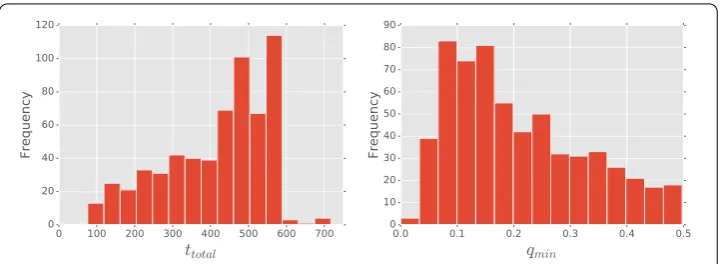
Figure 1 Population statistics.Left panel: the distribution of the number of days that the participants took part in the experiment. Right panel: the distribution of the fraction of missing data fort= 15 min.

consists of≈.·_{data points. The data was collected from February  up to March}

of , thus covering a multi year span with a substantial fraction participating for more than a year (see left panel of Figure ). Each data point consists of latitude and longitude coordinates, together with a timestamp and the accuracy associated with the measure-ments. These are converted into appropriate time series (see Mobility sequences and pre-dictability for details), and the fraction of bins with unknown locations is denotedqmin.

For our analysis we needqmin≤%(see Methods). This reduces the number of

partici-pants with suﬃcient data to . The right panel of Figure  shows the distribution ofqmin

at the lowest temporal scale ( minutes).

Mobility sequences and predictability. The raw GPS data needs to be ﬁltered and con-verted into a history of discrete locations, Ti, before the limits of predictability can be

determined. This can in principle be done in an inﬁnite number of ways, meaning that the GPS trace from a participant can give rise to many diﬀerent time seriesTidepending on

the ﬁltering and mapping chosen. In this work we convert the raw data into two diﬀerent time series:

– Tbins

i : Series of time bins.

– T_iloc: Series of locations.

A detailed description of the ﬁlters and mappings are given in the Methods section. An illustration of the conversion from GPS-trace intoT_ibins is shown schematically in Figure . The two dimensional space is covered by a grid with a grid length given bys. Each square in the grid is represented by a symbol, such that a human trajectory may look like this

T_ibins= [A,B,B,A,A,A,C, . . .]. ()

Each symbol corresponds to the grid cell position of a time bin of lengtht. The construc-tion of this trajectory is equivalent to that of earlier works [, , –]. As noted earlier, it depends on the spatiotemporal resolution and includes stationarity.

Next we introduce the new mobility encodingTloc

i , which aims to describe trajectories

(4)

Figure 2 Converting the raw data for participantiinto a suitable time series,T_ibins.After ﬁltering we plot the data points onto a world map overlaid with square grid cells with side lengthss. This converts each data point into alocationrepresented by a square grid cell and encoded by a symbol inTbins

i . The location

data is then resampled such that each bin inTbins

i corresponds to a time intervalt. This mobility encoding is

similar to that of earlier works and corresponds to the location in a sequence of time bins. We propose to look at a the sequence of locations instead.

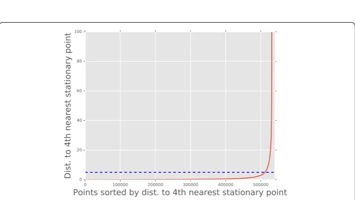
Figure 3 Choosing a length scale.We show the sorted distance to the fourth nearest stationary point for a subset of the entire data set. Standard methods [27] propose setting the parametervicinityequal to the distance where there is a sharp increase in the distance to the fourth nearest stationary point. Here we choose

= 5 meters as indicated by the dashed line.

of the individual. We then use a clustering algorithm (DBSCAN []) on the stationary data points to determine the diﬀerent locations automatically. This approach results in locations, which better represent the places where individuals spend their time, than the more commonly used Voronoi or square grid cells.

The clustering algorithm takes a length scale as input, which determines whether or not a stationary data point belongs to a location cluster. Here we usevicinity=  meters

(5)

We can now construct the trajectory of an individual among his/her locations, using the clusters found by the DBSCAN algorithm. In this encoding we do not include the time spent at the diﬀerent locations, but represent each location by just a single symbol, e.g.:

T_iloc= [A,B,A,C, . . .]. () Compare this with the sequence in () and note that the stationarity has been removed, i.e. no similar symbols in a row.

We expect the sequence of locations to be less predictable than the sequence of time bins, since it encompasses the more complicated spatial dynamics. In order to quantify this intuition, we need a measure of predictability. Here we use a slightly modified version of the scheme developed by [] (see Methods for details). First, the entropy rate of the mobility sequence is determined using an estimator based on the Lempel-Ziv compression algorithm. Since all the sequences are affected by missing data, one must extrapolate the entropy rate from missing data to full data. By testing our extrapolation on periods with complete data, we find that we can predict the true entropy within %, even when % of the sequence is missing. Having estimated the entropy rateHestwe are in a position to

determine the upper limit of predictabilitymax_{. This is done by solving []}

Hest= –maxlog

max– –maxlog_ –max+ –maxlog_(N– ), () whereNis the number of unique locations in the time series. The upper limit found repre-sents a tight upper bound attainable by an appropriate, but for now unknown, algorithm.

We also examine the lower limit of predictability. For the location sequenceTloc

i , we use

a ﬁrst order Markov chain to predict the next location [], i.e. we expect the location that most often follows the current location. If the current location has not been explored before, then we expect the most visited location as the next one. For the time bin sequence

Tbins

i we use a simple predictor, which expects the current location to continue into the

next time bin. This predictor will be referred to as “the trivial predictor” and it measures the amount of stationarity in the mobility sequence.

3 Results

We start by presenting our results forTbins

i , i.e. the mobility encoding that people have

been using previously. As noted earlier, the predictability of these sequences depend on the spatiotemporal resolution. In the left panel of Figure  we ﬁxs=  m and varytto determine how the upper and lower limits depend on the temporal scale. The predictabil-ity grows towards  as the time scale is decreased, just as expected by our conjecture (). Note the high performance of the trivial predictor (%-%).

(6)

Figure 4Next binpredictability depends on spatiotemporal resolution.Left panel: The temporal resolution dependency of the upper limits (squares) and lower limits (discs) of predictability for the next bin approach. Each location is represented by a square grid withs= 400 m. Error bars are included but are smaller than the symbols. Right panel: The spatial dependency at a ﬁxed temporal resolution oft= 15 min. The lower limit shows that, depending on resolution, 85% to 94% of the predictability is due to peoplenot

moving.

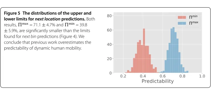
Figure 5 The distributions of the upper and lower limits fornext locationpredictions.Both results,max_{= 71.1}_±_{4.7% and}min_{= 39.8}

±5.9%, are signiﬁcantly smaller than the limits found fornext binpredictions (Figure 4). We conclude that previous work overestimates the predictability of dynamic human mobility.

The limits presented in Figure  follow our postulate and are in agreement with earlier works with smaller populations. We now test what happens when we remove the stationar-ity from the spatial dynamics, i.e. when we consider the predictabilstationar-ity of the next location instead. In Figure  we show the distributions of the upper and lower limits for next lo-cation predictability. Both limits are strongly reduced when compared to the results for next bin predictability. For the upper limit we ﬁndmax_{= .}_±_._%_{, i.e. a signiﬁcant}

reduction from the >%predictability found in previous works. We ﬁnd that this value is very robust to increases in the length scale and that it only changes by a few percent as

is increased towards  meters. The lower limit is found to bemin_{= .}_±_._%_{, which}

is at least %lower than any of the lower limits found by the trivial predictor for next bin sequences.

We note that another group has simultaneously been working on the same data set with the same methods and they have foundmax_{= . []. Despite the close match in results}

they have actually been using very diﬀerent DBSCAN paramters, namelyvicinity=  (we

use vicinity= ) and min_pts =  (we use min_pts = ), thereby further underlining the

(7)

Table 1 Examining which factors impact the predictability of human mobility patterns.rgis

the radius of gyration,eﬀ_placesis the effective number of places an individual chooses from when changing to a new location and is deﬁned as 2Hunc_{. We also examine the impact of basic}

personality traits using the Big Five psychological proﬁle [30]. Error bars are determined using the bootstrap method

Measure Correlation withmax

rg –0.05±0.05

eﬀplaces –0.26±0.05

min 0.49±0.04

Agreeableness –0.05±0.06 Conscientiousness 0.04_±0.06 Extroversion –0.13±0.05 Neuroticism 0.06±0.06 Openess –0.004±0.059

The above results raise the question: what factors impact the predictability of human mobility? Our partial answer to this question can be found in Table , where we correlate

maxto a range of variables. We ﬁnd that radius of gyration, representing typical distances traveled, does not impact next place predictability. A related result has been reported ear-lier, using next bin predictability []. While this result can seem counterintuitive, our next result is able to shed more light on the matter.maxis anti-correlated with the eﬀective

number of places an individual chooses from, when determining where to go next. There-fore, the predictability of an individual does not depend on the reach of his/her travels, but rather on the number of places visited.

Finally, utilizing the psychological profiles of the participants, we are able to examine the impact of their psychological traits on their predictability. The only significant corre-lation we find here is with extroversion, meaning that the next location of an extroverted individual is statistically harder to predict.

4 Conclusion

Our results show that it is possible to extract a wide range of upper and lower limits of pre-dictability of human mobility depending on the ﬁltering and discretization scheme cho-sen. We have shown the strong dependency of “next bin” predictability on spatiotemporal scales. Furthermore, we have shown that the predictability at large spatial scales and small temporal scales mostly reﬂect stationarity, namely that people stay in the same spatial bin. This raises the need for an alternative approach to estimate the predictability of human mobility patterns.

The task of predicting human mobility is two fold: how long will a person stay in a cer-tain location and where they will go next. Here we determined an upper limit on the pre-dictability of the latter. We found that the upper limit of this task is much lower than the previously stated ones of∼%. In particular, by using the natural length scale of human locations we found an upper limit on predictability of .±.%. A lower limit was like-wise found using a ﬁrst order Markov chain model with a success rate of .±.%. Overall, our results indicate that it might not be so trivial to predict human mobility after all.

5 Methods

(8)

char-acterized by two parameters: a length scale sand the origin of the map. The Techni-cal University of Denmark, where most of the participants were enrolled, was chosen as the origin. This ensured that the grid cells had sides of approximately equal length

s at the locations where most of the data was collected. The length scales used are

s∈[, , , , ] meters.

Small changes in the origin of the grid map can effect the number of locations detected []. To mitigate the possible bias introduced by having a fixed origin of the grid map, we add a random offset for each participant chosen randomly from a uniform distribution on [,s].

Our data was not sampled at a ﬁxed rate. A time binning with a ﬁxed temporal resolution

tallowed us to convert the raw data into a time series. The binning is done such that for each time bin we chose the most visited location. If two or more locations are the most visited locations, then we chose one of them at random. The time scales used aret∈

[, , , , ] minutes. Time bins with no recorded locations are denoted using a special ? marker. Thus we end up with a time seriesT_ibinswhich depends primarily ons

andt.

Converting the raw data into Tloc

i . Again we start by employing the accuracy ﬁlter. To

reduce the number of data points associated with travel, we employ a second filter inspired by thepause-basedmodel used in []. It detects all the data points which are ±. min apart and for which the distance between the two measurements are less than  m. These two measurements are then averaged into a single data point representing a place where a participant stood still for roughly a quarter of an hour. This filters out most of the travel information in the dataset, except interruptions such as traffic jams and waiting for public transport.

The list of locations is binned with a ﬁxed temporal resolutiont=  min as described above. After this we compress every time series such that all instances where a participant stood still for more than one time bin are represented by just a single symbol. This is best explained by an example. A time series obtained by the procedures described above could look like:Ti= [A, ?,A,B,B,A,A,A,C, . . .]. After compression this time series is converted

into:

T_iloc= [A,B,A,C, . . .]. ()

The resulting time series are independent oftprovided thattis small. The smallest sampling rate that we dare use in this study ist= , since smaller sampling rates would make it diﬃcult to distinguish stationarity from movement because of the limited accuracy of the GPS.

Estimating the entropy rate.The entropy rate is found using an estimator based on the Lempel-Ziv compression algorithm []:

Hrate=



n·

n

i=

i log(n)

–

, ()

wherenis the length of the time series andiis the length of longest substring in the time

(9)

The fraction of missing data,q, changes the entropy rate estimate. By artiﬁcially re-moving data in complete records we can study possible extrapolation methods. We have used a subset of  individuals with a complete location record spanning at least  weeks. For each of these complete records we determinedHtrueusing the estimator ().

Remov-ing data from these complete records and comparRemov-ing the entropy rate determined by our method,Hest, withHtrue, we found that we could estimateHtruewithin±%as long as

q≤.. Our method is thus able to determine the entropy rate even when we only know half of the locations visited. Earlier this method has been used up toq≤. [], but our tests show reliable results only whenq≤..

Our extrapolation works as follows. For each time series we determine the amount of time the participants location was unknown. This fraction of the total time was de-notedqmin. We then found bothHunc(q) andHrate(q) for eachq∈[qmin,qmin+ .,qmin+

., . . . , . –qmin]. Here Hunc is the entropy of the time series, found using Hunc =

–N_i_=pilog(pi), where the sum runs over all theNdiﬀerent locations visited andpiis

the fraction of time spent ati. This enabled us to calculateσ(q) =Hrate(q)/Hunc(q).

Ear-lier it has been shown [] that σ(q) depends linearly onq. This linear relation has not been found when using data with a higher sampling rate []. Our set of complete records showed thatσ(q) could be fitted well with an offset exponential function. Using these fits we could extrapolate and determineσest=σ(q= ). The entropy rate was then found using

Hest=expσest·Hunc(q). ()

Funding

The study received funding through the UCPH 2016 Excellence Programme for Interdisciplinary Research.

List of abbreviations

GSM: Global System for Mobile Communications GPS: Global Positioning System

DBSCAN: Density-based spatial clustering of applications with noise

Availability of data and materials

Data are part of larger study “Social Fabric” involving researchers at the Technical University of Denmark and University of Copenhagen. Due to privacy consideration regarding subjects in our dataset, including European Union regulations and Danish Data Protection Agency rules, we cannot make all data used here publicly available. The data contains detailed information on mobility and daily habits at a high spatio-temporal resolution. We understand and appreciate the need for transparency in research and are ready to make the data available to researchers who meet the criteria for access to conﬁdential data, sign a conﬁdentiality agreement, and agree to work under our supervision in Copenhagen.

Ethics approval and consent to participate

The “Social Fabric” study was reviewed and approved by the appropriate Danish authority, the Danish Data Protection Agency (Reference number: 2012-41-0664). The Data Protection Agency guarantees that the project abides by Danish law and also considers potential ethical implications. All subjects in the study gave written informed consent.

Competing interests

The authors declare that they have no competing interests.

Authors’ contributions

Conceived and designed the study: EI AM. Analyzed the data: EI. Wrote the paper: EI AM.

Publisher’s Note

Springer Nature remains neutral with regard to jurisdictional claims in published maps and institutional aﬃliations.

Received: 19 September 2016 Accepted: 4 June 2017 References

(10)

3. Song C, Qu Z, Blumm N, Barabási AL (2010) Science 327(5968):1018

http://science.sciencemag.org/content/327/5968/1018. doi:10.1126/science.1177170

4. Qian W, Stanley KG, Osgood ND (2013) In: Web and wireless geographical information systems. Springer, Berlin, pp 25-40

5. Rhee I, Shin M, Hong S, Lee K, Kim SJ, Chong S (2011) IEEE/ACM Trans Netw 19(3):630 6. Song C, Koren T, Wang P, Barabási AL (2010) Nat Phys 6(10):818

7. Jiang S, Yang Y, Gupta S, Veneziano D, Athavale S, González MC (2016) Proceedings of the National Academy of Sciences p 201524261

8. Pappalardo L, Simini F (2016) arXiv preprint arXiv:1607.05952

9. Barbosa H, de Lima-Neto FB, Evsukoﬀ A, Menezes R (2015) EPJ Data Sci 4(1):21

10. Pappalardo L, Simini F, Rinzivillo S, Pedreschi D, Giannotti F, Barabási AL (2015) Nature communications 6 11. Toole JL, Herrera-Yaqüe C, Schneider CM, González MC (2015) J R Soc Interface 12(105):20141128 12. Colizza V, Barrat A, Barthelemy M, Valleron AJ, Vespignani A (2007) PLoS Med 4(1):e13

13. Kleinberg J (2007) Nature 449(7160):287

14. Gabaix X, Gopikrishnan P, Plerou V, Stanley HE (2003) Nature 423(6937):267

15. Pappalardo L, Vanhoof M, Gabrielli L, Smoreda Z, Pedreschi D, Giannotti F (2016) Int J Data Sci Anal 2(1-2):75 16. Frias-Martinez V, Virseda J (2012) In: Proceedings of the ﬁfth international conference on information and

communication technologies and development. ACM, New York, pp 76-84 17. Makse HA, Andrade JS, Batty M, Havlin S, Stanley HE et al (1998) Phys Rev E 58(6):7054 18. Kitamura R, Chen C, Pendyala RM, Narayanan R (2000) Transportation 27(1):25 19. Krings G, Calabrese F, Ratti C, Blondel VD (2009) J Stat Mech Theory Exp 2009(7):L07003 20. Ranjan G, Zang H, Zhang ZL, Bolot J (2012) Mob Comput Commun Rev 16(3):33 21. Lin M, Hsu WJ (2014) Pervasive Mob Comput 12:1

22. Jensen BS, Larsen JE, Jensen K, Larsen J, Hansen LK (2010) In: Machine learning for signal processing (MLSP), 2010 IEEE international workshop on. IEEE, New York, pp 196-201

23. Smith G, Wieser R, Goulding J, Barrack D (2014) In: Pervasive computing and communications (PerCom), 2014 IEEE international conference on. IEEE, New York, pp 88-94

24. Lin M, Hsu WJ, Lee ZQ (2012) In: Proceedings of the 2012 ACM conference on ubiquitous computing. ACM, New York, pp 381-390

25. Stopczynski A, Sekara V, Sapiezynski P, Cuttone A, Madsen MM, Larsen JE, Lehmann S (2014) PLoS ONE 9(4):e95978 26. Pedregosa F, Varoquaux G, Gramfort A, Michel V, Thirion B, Grisel O, Blondel M, Prettenhofer P, Weiss R, Dubourg V,

Vanderplas J, Passos A, Cournapeau D, Brucher M, Perrot M, Duchesnay E (2011) J Mach Learn Res 12:2825 27. Tan PN, Steinbach M, Kumar V (2005) Introduction to data mining. Pearson, Upper Saddle River 28. Lu X, Wetter E, Bharti N, Tatem AJ, Bengtsson L (2013) Scientiﬁc reports 3

29. Cuttone A, Lehmann S, González MC (2016) arXiv preprint arXiv:1608.01939 30. Digman JM (1990) Annu Rev Psychol 41(1):417