A R T I C L E
DOI 10.1007/s12651-017-0218-4
Identifying couples in administrative data
Deborah Goldschmidt1· Wolfram Klosterhuber2· Johannes F Schmieder3,4,5,6,7
Accepted: 10 January 2017 / Published online: 15 May 2017 © The Author(s) 2017. This article is an open access publication.
Abstract We develop a new method for identifying mar-ried couples in administrative data. Using address and name data from the universe of employment records in Germany we find around 3.3 Mio. pairs of individuals who are living at the same location, have a matching last name and are less than 15 years apart in age. We show supporting evidence that around 89 to 94% of these pairs are indeed married couples and provide careful consistency checks. Using in-formation from the German Microcensus, we show that our method identifies about 17% of all married couples in Ger-many and about 35% of couples where both spouses are in social security covered jobs or unemployed. In ongoing work this couple identifier will be made available to the research community and users for the IAB administrative data. Our method thus opens the door for household level analyses benefiting from the precision and very large num-ber of observations available in administrative data.
Keywords Couples · Geocoding · Administrative data · Household analysis
Johannes F Schmieder [email protected]
1 Analysis Group, New York City, USA 2 IAB, Nuremberg, Germany
3 Department of Economics, Boston University
College of Arts & Sciences, 270 Bay State Road, Boston, Massachusetts 02215, USA
4 NBER, Cambridge, USA 5 IZA, Bonn, Germany 6 CESIfo, Munich, Germany 7 CEPR, London, United Kingdom
JEL Code J12
Identifizierung von Ehepaaren in Administrativen Daten
Zusammenfassung Wir entwickeln eine neue Methode zur Identifizierung verheirateter Paare in administrativen Daten. Mittels Adressdaten und Nachnamen der Gesamt-heit der Beschäftigungsmeldungen in Deutschland, identi-fizieren wir ca. 3,3 Millionen Paare von Personen die an der gleichen Adresse wohnen, deren Nachnamen überein-stimmen, und einen Altersabstand von weniger als 15 Jah-ren haben. Wir zeigen mittels verschiedener Konsistenz-checks, dass ca. 89 bis 94 Prozent dieser Paare tatsäch-lich verheiratete Paare sind. Anhand von Informationen des Mikrozensus, zeigen wir, dass unsere Methode etwa 17 Pro-zent aller verheirateten Paar in Deutschland identifiziert und ca. 35 Prozent aller Paare bei denen beide Partner in so-zialversicherungspflichtiger Beschäftigung oder arbeitslos sind. Der Paarindikator wird der Forschungsgemeinschaft und Nutzern der IAB Daten zur Verfügung gestellt. Unsere Methode eröffnet damit neue Forschungsmöglichkeiten für Haushaltsanalysen die von der Präzision und großen Beob-achtungszahlen von administrativen Daten profitieren.
1 Introduction
follow the units of observation over time and the high qual-ity of recorded information. This shift has been particularly forceful in Labor and Public Economics, where the avail-ability of individual level employment and tax records has led to the rise in new research designs such as regression discontinuity, regression kink or bunching designs that rely on very large sample sizes. While administrative data offer many advantages, they also come with limitations and the scope of available variables is often quite limited compared to household surveys. In particular, administrative employ-ment records are typically on the individual level only and it is often not possible to link individuals to other house-hold members. For this reason, administrative data have played a smaller role in studying traditional questions in la-bor economics, such as household lala-bor supply, household investment decisions in human capital or within household income differences.1
In this project we develop a new method to impute house-hold identifiers in the administrative employment records data in Germany to increase the scope of research ques-tions that can be addressed. Our approach is to identify pairs of individuals who are, with a high probability, mar-ried couples using information on addresses, family names and dates of birth. In Germany it is still very common that at the time of marriage one spouse (in the vast majority of cases the wife) adopts the other spouse’s last name, ei-ther fully or as part of a double name. If two individuals with matching last names are living together at the same address, they are likely related, though they could also be in a sibling or parent-child relationship. To further narrow it down to married couples we take pairs of a woman and a man with matching last names with an age difference of less than 15 years, which should exclude most parent-child relationships. We present a detailed analysis of the likely extent of errors when applying this method. The new identi-fiers for married couples will be made available to external researchers and users of the IAB administrative datasets, facilitating a broad range of possible research projects that rely on household/couple identifiers. Something to which we return to in the conclusion.
Germany has a long tradition of women taking on their husbands’ last name at the time of marriage. The German Civil Code from 1896 unequivocally required that the wife takes on the name of her husband.2 A reform in 1953
al-1 While some countries do allow for linking households in their
admin-istrative registry data, resulting in exciting and influential work, these countries tend to be relatively small and geographically clustered, such as Austria (Frimmel et al.2014) or the Scandinavian countries (e. g. Hardoy, and Schøne2014or Huttunen and Kellokumpu2016). Ex-panding the scope of administrative data to other countries will be very valuable to study the household behavior in new contexts.
2 See Sperling (2012) for a discussion of the legal history of the family
name law in Germany.
lowed for the wife to keep her birth name as part of a dou-ble (or hyphenated) last name, but she was still required to take on her husband’s name as the family name. The family name law was revised again in 1970 allowing that a cou-ple could decide to take on the wife’s name as the family name, but kept the requirement of a common family name for both spouses. Furthermore, if a couple could not come to an agreement with respect to which name would become the family name the decision was up to the husband. This only changed with a decision by the German constitutional court in 1991 and a subsequent revision of the family name law in 1994, after which both spouses were allowed to keep their own birth names, while the traditional option of taking on one of the birth names or a hyphenated double name for one of the spouses continued to exist. In practice it appears that it is still the case that the vast majority of women take on their husband’s names either fully or at least as part of a double name. While we are not aware of representative surveys or official registry data for Germany that would al-low us to calculate the share of couples with matching last names, we found various press reports from city level wed-ding registries that seem to suggest that even among newly wedded couples around 85 to 90% still have a matching last names.3 Among couples married for longer (and in
partic-ular before 1994), the ratio is likely significantly higher. We implement the method of identifying likely couples using last names, addresses and age using a cross-section of the administrative data from the Institute for Employment Research (IAB) in Germany spanning the universe of em-ployment and unemem-ployment records for 2008. This data, called Integrated Employment Biographies or IEB, covers all individuals who are employed in employment subject to social security contributions, receive benefits from the un-employment insurance (UI) system, or who are registered as job seekers. This data covers around 80% of employ-ees, in particular excluding public servants and the self-employed. By design we are only able to identify married couples where both spouses are covered in the IEB. While this is certainly not a representative sample and excludes a sizable part of the population of couples we are still able to identify over 3 Mio. couples who are likely married to each other.
The two main concerns with this approach are the poten-tial for false positives and false negatives. False positives may arise because people with matching last names may live at the same address either purely by chance, or
be-3 All-in (2006) report that in Kempten in 2006 around 14% of newly
cause they are related to each other but not married. Using the distribution of same-sex matching name pairs, as well as information on family status for a subset of individuals we show that likely around 88–94% of our sample of cou-ples are indeed married to each other. Even if both spouses of a married couple are in our data, false negatives may arise, because we may not match them to each other. Either they do not have matching names or there are more than 2 matching individuals at a location, making it impossible to tell who is married to whom. False negatives will also arise whenever one or both members of a marriage are not covered in the IEB data, which for example would include all self-employed, public servants or individuals not in the labor force, but also all individuals older than age 65. Us-ing information from the Microcensus, we show that we can identify roughly 20% of the 19 Mio. married couples in Germany. Furthermore, we identify about one third of married couples where both individuals are covered by the IEB data (i. e. working in social security covered job or un-employed). We compare observable characteristics of our matched couples with the official microcensus data to show how our sample differs from the general population of mar-ried couples. While the representativeness of the matched couples is clearly limited, many research questions do not rely on having a representative sample. The large number of observations and the possibility to observe complete em-ployment histories in the IAB data should make this data a valuable tool for many research projects. We will return to a discussion of how this data can be used in the conclusion. This paper is related to other research that uses the special features of administrative data to impute informa-tion that is not directly available. For example, Jacobson, Lalonde and Sullivan (1993) use the combination of individ-ual and firm identifiers in UI records from Pennsylvania to impute plant closings and mass-layoffs by observing when large numbers of individuals are moving away from firm identifiers and are scattered across many other employers. Hethey-Maier and Schmieder (2013) use a similar approach to identify new plant openings in administrative data, rely-ing on worker flow information to distrely-inguish plant open-ings from spurious changes in firm identifiers. Goldschmidt and Schmieder (2015) identify outsourcing of labor services in large firms employing an algorithm based on a combina-tion of worker flows, industry and occupacombina-tion codes.
The next section describes the data used in this project. Sect. 3 describes our method for identifying couples and presents the results based on individuals in 2008. In Sect. 4 we show supportive evidence that our method does in fact largely identify married couples and develop bounds on the fraction of false positives. We then present characteristics of the couples that we identify with our method and compare them to the general population in the German employment data, as well as to other data sources. Sect. 5 concludes.
2 Data sources
In this chapter, the sources of the data are explained in detail. Sect. 2.1 describes the Integrated Employment Bi-ographies (IEB) data, while the geocoded location data and the individual name data are discussed in 2.2 and 2.3.
2.1 Integrated employment biographies
The IEB of the Institute for Employment Research stem from the notification process of the social security system of the Federal Employment Agency (BA). The IEB is the basis for most of the widely used research datasets provided by the IAB to the research community, such as the SIAB data, the LIAB data, the BHP and many others. The IEB consolidate completed, historicized and edited process data from different data sources, which come from different op-erative systems. It comprises all persons registered with the Federal Employment Agency due to the following:
● Employment subject to social security or marginal part-time employment.
● Receipt of unemployment insurance benefits in accor-dance with Social Code Book II or III.
● Job search registered with local employment agencies. ● Planned or actual participation in an employment or
training programs.
The IEB includes demographic variables such as nation-ality, birthdate, gender, and education. Information on em-ployment, benefit receipt and job search include daily wage, daily benefit rate, occupational and employment status or economic activity. Additionally location data such as place of residence or work on different aggregated levels are pro-vided. There were around 35 Mio. working individuals in Germany in 2008 (own calculations based on Microcensus data), about 80% of whom have at least one record in the IEB. The biggest groups which are not included in the bi-ographies are self-employed workers and public servants calledBeamte.4
We also have information on family status (married, liv-ing alone, sliv-ingle parent, cohabitatliv-ing), but only for the sub-set of individuals who are unemployed and registered as job seekers. We use this information in Sect. 4 for various consistency checks.
2.2 Geocoded data
Our method relies on finding individuals living at the same location. In principle individuals can be matched to other individuals at the same location either by directly com-paring addresses, or by first geocoding addresses into
tude/longitude coordinates and then comparing coordinates. Matching addresses directly is complicated by the fact that these can often be written in a variety of ways and need to be carefully cleaned. We instead match individuals on geographic coordinates, where the address processing was done using GIS software, which allows for careful error correction methods. The geocoding was done in a project between the Research Data Centre (FDZ) and the Univer-sity of Duisburg-Essen for a cross-section of all individuals in the IEB data as of June 30th, 2008. This project used data from the Federal Agency for Cartography and Geodesy, and includes 22 Mio. addresses of German buildings and their geographic coordinates and it was possible to successfully geocode 94.6% of the IEB records.5Individuals whose
ad-dresses are not geocoded were dropped from the data and are not used in the further analysis.
2.3 Names
One of the criteria that we use for determining couples is whether the last names of two people match. We therefore also obtained data on last names covering the universe of individuals who have a record in the IEB as of June 30th, 2008. In order to improve the probability of success in matching, we first clean the names of errors and typos, and ensure consistency in terms of special characters and titles. With the support of the German Record Linkage Centre (GermanRLC) and their algorithm, the names of the indi-viduals were cleaned, taking into account certain patterns and potential discrepancies.6Umlauts were substituted (ä!
ae and so forth) as well as ß to ss. All blank spaces in the front, middle or end of the name were removed. Profes-sional and nobility titles (such as Dr., Prof., Freiherr von) were removed as well, and special characters (e. g. ~ or %) and non-ASCII characters (e. g. © or ™) were deleted.
The only special character that was retained is the hy-phen (-), which is used to indicate double names. While the family name law in the civil code book states that a spouse can add their birth name to the family name does not specif-ically mention a hyphen, in practice this appears to be the only option. In fact a court decision from 2013 specifically ruled that a couple was not allowed to combine the birth names of two spouses without a hyphen (Kammergericht Berlin2013). Furthermore individuals are not allowed to create last name chains that involve more than one hyphen (for example if at the time of marriage an individual already
5 See Scholz et al. (2012). That paper is based on geocoded data from
2009, but 2008 was also geocoded as part of the same project. We de-cided to use 2008 as a baseline to allow for more analysis years after the couples are identified which seemed useful for many possible research questions. In the future we hope to expand the procedure to more years.
6 See for example Schild and Antonio (2014) p. 4 ff.
has a double name from a previous marriage). We thus as-sume that double names are always separated by a hyphen and we describe below how we use hyphenated names in our name-matching algorithm. At the end of the cleaning process all letters were converted to upper case.
Although individuals have a consistent personal iden-tifier, the Einheitliche Statistische Person (ESP), the last name may vary across different data sources. If, after the name cleaning process was completed, discrepancies per-sisted in the names across data sources, the individual was dropped. The exception was when an individual had a dou-ble last name in one source and an overlapping single last name in another (e. g. MUELLER-MEIER in one source and MEIER in another). In this case, the double last name was kept.
3 Identifying couples
As mentioned previously, although the IEB data consists of a large amount of information on the majority of the German population, it – like many administrative data sets – does not include any information on the household. To circumvent this issue, we combine the IEB data with the geocoded location data and information on names to infer probable married couples. We use the following criteria to ensure that the matches we identify are most likely married couples and not simply two people with some other type of relationship (or no relationship at all):
1. Same home location.
2. Uniquely matching last name.
3. One male, one female, with an age difference of less than 15 years.
We go into more detail on each of these requirements below.
3.1 Location
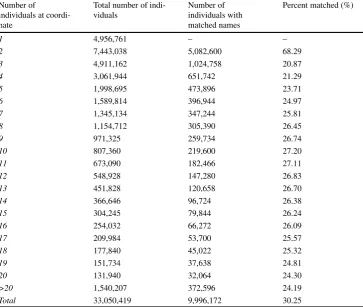
The first step in identifying potential married couples is finding people who live at the same location, since most married couples live together. We start by looking at the distribution of the number of individuals at a particular lo-cation, using each person’s geocoded coordinates, for the ~33 Mio. people in our data. The second column of Table1
Table 1 Distribution of the Number of Individuals at the Same Coordinate
Number of
individuals at coordi-nate
Total number of indi-viduals
Number of individuals with matched names
Percent matched (%)
1 4,956,761 – –
2 7,443,038 5,082,600 68.29
3 4,911,162 1,024,758 20.87
4 3,061,944 651,742 21.29
5 1,998,695 473,896 23.71
6 1,589,814 396,944 24.97
7 1,345,134 347,244 25.81
8 1,154,712 305,390 26.45
9 971,325 259,734 26.74
10 807,360 219,600 27.20
11 673,090 182,466 27.11
12 548,928 147,280 26.83
13 451,828 120,658 26.70
14 366,646 96,724 26.38
15 304,245 79,844 26.24
16 254,032 66,272 26.09
17 209,984 53,700 25.57
18 177,840 45,022 25.32
19 151,734 37,638 24.81
20 131,940 32,064 24.30
>20 1,540,207 372,596 24.19
Total 33,050,419 9,996,172 30.25
Second column includes all geocoded data as of June 30th 2008. Third column includes all individuals with geocoded location for whom we were able to match according to our name-matching algorithm, described in the text
the dataset; as the number of people living at a coordinate gets larger, the absolute number of people living in this type of residence decreases.
3.2 Names
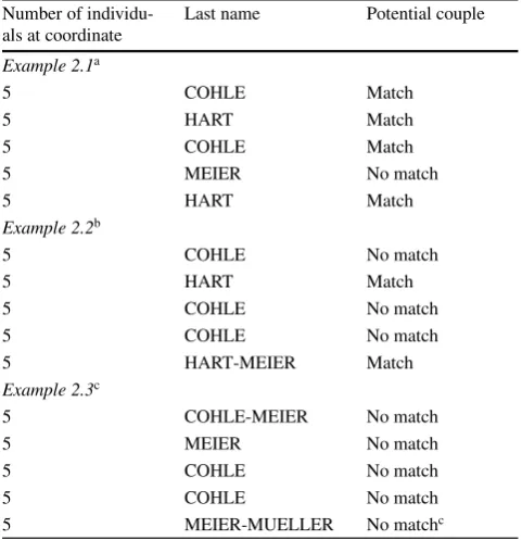
Next, we look at the cleaned names of the individuals liv-ing within any given location. We require that our identified married couples share a last name. In situations where any of the people in the location has a hyphenated name, we consider two names to be a match if at least one part of the hyphenated name is identical to another name at the location. In locations with multiple people, we addition-ally require that a maximum of two people have matching names. Otherwise, we have no way to determine which two individuals are likely to be a couple and which may be un-related, or related in other ways. The following examples help to clarify the procedure.
In Example 2.1 (Table2), there are 5 individuals living at a particular coordinate. Two have the last name COHLE, and there are no others named COHLE at this location, so they are kept as a potential match. Two are named HART, with no others named HART, and so they are also kept as a potential match. Finally, there is a single person named
MEIER, who is dropped from our potential group of cou-ples. In Example 2.2 (Table2), we again have 5 individu-als living at the same coordinate: three have the last name COHLE, one has the last name HART, and one has the last name HART-MEIER. Because there are more than 2 indi-viduals at this location with the last name COHLE, we can not be certain which of these are part of a couple and which are not, so we drop all three. Because HART and HART-MEIER share a partial name, even though one is hyphen-ated, they are kept as a potential match. In Example 2.3 (Table 2), there are again 5 individuals at the same coor-dinate. Because COHLE, COHLE and COHLE-MEIER all match in terms of their names, we must eliminate all three, since we have no way of knowing which two could really be a couple. Similarly, MEIER, MEIER-MUELLER and COHLE-MEIER must all be dropped, despite their names matching. Therefore, in this example, there is no match chosen.
Table 2 Examples of the name-matching procedure Number of
individu-als at coordinate
Last name Potential couple
Example 2.1a
5 COHLE Match
5 HART Match
5 COHLE Match
5 MEIER No match
5 HART Match
Example 2.2b
5 COHLE No match
5 HART Match
5 COHLE No match
5 COHLE No match
5 HART-MEIER Match
Example 2.3c
5 COHLE-MEIER No match
5 MEIER No match
5 COHLE No match
5 COHLE No match
5 MEIER-MUELLER No matchc
These are provided as examples only, and are not taken from the actual data amatches HART and COHLE are chosen
bmatch (HART-)MEIER is chosen cno match is chosen
with only 2 individuals, almost 70% had matching names. At coordinates with 3 or more people found at the same location, the match rate is between 20 and 30%.
There are several limitations to this criterion. First, while the majority of married couples in Germany share a last name (or part of a double name), not all women (or men) change their last name upon marriage, and we are certain to miss those couples. Second, in locations with multiple people where more than two share a last name, since we can not be certain which two members are married (if any) we must drop them all, eliminating more potential matches from our sample. Finally, we may be capturing two peo-ple with the same last name living in the same coordinate who are related but not married. In addition, particularly in multi-unit residences, there may be two people who are unrelated but have the same last name, and we may erro-neously be including them in our sample. Our next criteria,
Table 3 Gender Composition of Matched Potential Couples
Matches All matches Age Difference <15 Age Difference≥15
Absolute Percent (%) Absolute Percent (%) Absolute Percent (%)
Male/female 4,084,516 81.72 3,281,657 94.65 802,859 52.44
Male/male 482,891 9.66 131,550 3.79 351,341 22.95
Female/female 430,679 8.62 53,763 1.55 376,916 24.62
Total 4,998,086 100.00 3,466,970 100.00 1,531,116 100.00 Includes all individuals with geocoded location for whom we were able to match according to our name-matching algorithm, described in the text
on gender and age, will eliminate some of these falsely matched people from our sample, but not all.
3.3 Gender and age
Finally, we take our set of potential couples – groups of two people who share a last name and a location – and impose gender and age restrictions. Since we are currently only identifying heterosexual couples, we require that each couple be composed of one male and one female, informa-tion that is available in the IAB records. The second column of Table3presents the gender composition breakdown for the 5 Mio. identified potential couples. More than 4 Mio. of these pairs consist of one male and one female, while the remainder is made up of either two males or two females. We drop the single-sex households and move on to the age difference requirement.
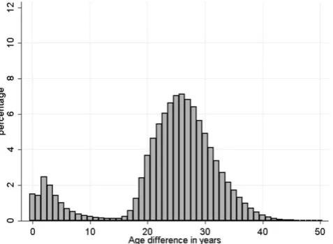
Fig. 1 Distribution of age differences of matches, male/female. (Note: Includes all male-female pairs of individuals who we were able to match by location and name (according to our name-matching algorithm). Age difference is calculated as man’s age – woman’s age)
Fig. 2 Distribution of age differences of matches, female/female. (Note: Includes all female-female pairs of individuals who we were able to match by location and name (according to our name-matching algorithm). Age difference is calculated as older age – younger age)
an age difference of 0–15 years; these may be siblings or other familial relationships, homosexual couples, or other pairs of people who coincidentally have the same last name in the same location. While homosexual couples can form a civil union in Germany since 2001 which allows them to adopt a common family name, these still seem to be rela-tively rare, with only 34,000 same sex civil unions in 2011 (Statistisches Bundesamt2012). Thus while a small part of the same sex matches might be same sex couples most of them are not. The fact that the number of same sex matched individuals in our sample is quite small, suggests that there are relatively few cases where people live together with the same last name for other reasons than being married to each other and that in turn most matched individuals who are
liv-Fig. 3 Distribution of age differences of matches, male/male. (Note: Includes all male-male pairs of individuals who we were able to match by location and name (according to our name-matching algorithm). Age difference is calculated as older age – younger age)
ing with each other in this age group are in fact married to each other.
For determining our sample of couples, we require that the difference in age of the matched man and woman be less than 15 years. This should eliminate any mother-son or father-daughter pairs from the set of couples. The re-maining pairs – consisting of one man and one woman, with matching last names, who live in the same location and are less than 15 years apart in age – make up our fi-nal sample. Columns 4–5 of Table3show the results when we impose our age difference restriction. We retain 80% of our male-female couples, leaving us with a final sample of about 3.3 Mio. couples. This sample should be primar-ily composed of true couples, although some share will be “false positives”, made up of male-female siblings or fam-ily members who are similar in age, or unrelated people with the same name living at the same coordinates.
4 Consistency checks
Errors in our matching algorithm could occur in two ways. First, we have false positives – two people who are matched to each other by our algorithm, but who are not really a mar-ried couple. Second, there are couples that we do not pick up with our matching method, for various reasons. We dis-cuss these two issues, and the steps we take to quantify their magnitude, below.
4.1 False positives
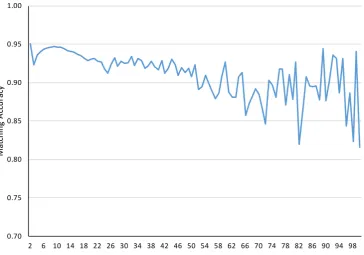
Fig. 4 Match Accuracy cal-culated based on Same-sex Matches by Number of Individ-uals living at same coordinate. (Note: In this figure we calcu-late the likely probability that a matched couple is indeed married to each other. For this we assume that the number of matched male/male and female/ female couples obtained by us-ing the same algorithm as for matched male/female couples is a proxy for the number of false matched. The accuracy can then be calculated as: [N(f/m) –N(f/f) –N(m/m)]/N(f/m). The figure plots this accuracy rate as a function of the number of individuals who live at the same coordinate where the couple is matched)
be wrongly matched if: (1) they are brother and sister, or have some other family relationship, are close in age, and live in the same location; or (2) they are unrelated, but living in a multi-unit residence, such as an apartment building, and happen to have the same last name and are close in age.
We can try to measure the size of this type of error in our final sample of couples in a few ways. First, we can use the distribution of same-sex matches to give us a sense of what share of our sample are wrongly matched if we make the following two assumptions. The first assumption is that opposite-sex family members who are close in age (i. e. brother and sister) are as likely to live together as same-sex family members (two sisters, for example). The second is that it is as likely for two people of the opposite sex who live in the same building to share a last name as it is for two peo-ple of the same sex. Using these assumptions, we can look at the number of same-sex matched pairs that fall within our age difference restriction (ages within 15 years of each other), using the numbers provided in Table3– these cou-ples are likely either pairs of family members living in the same location, or unrelated people with the same last name in the same building. We find that there are 185,313 male/ male and female/female pairs that fall within our age restric-tion. So, it is likely that approximately 185,000 couples in our sample of matched male-female couples with age differ-ence under 15 years are also wrongly matched. In fact, since there are some same-sex civil unions where partners share a family name, this arguably overestimates the number of
false positives by a small amount.7Using this methodology,
our accuracy rate is around 94% (final sample is 3,281,657; estimated wrongly matched is 185,313; correctly matched = 3,281,657– 185,313 = 3,096,344; accuracy rate = correctly matched/final sample = 3,096,344/3,281,657 = 94%). So, according to this method, only about 6% of our sample is wrongly matched and our sample does indeed identify cou-ples who with a high degree of certainty are indeed married to each other.8
We can also use this approach to get a sense of whether the accuracy of matches varies by the number of individuals living at the same coordinate. Intuitively in large apartment buildings with many units it is more likely to have two indi-viduals with matching last names who are unrelated. Fig.4
shows the match accuracy by the number of individuals at the same coordinate. The accuracy rate is clearly the highest at coordinates with just 2 individuals with a match accuracy rate of 95%. At coordinates with 3 individuals the match
7 Statistisches Bundesamt (2012) states that there are about 34,000
same sex civil unions in Germany in 2011. We do not know how com-mon it is for same sex couples to adopt a comcom-mon family name, nor that they would both be employed and covered in our data. It appears that due to the small number of same sex civil unions our method for identifying male-female marriages would not work as well for identi-fying same sex civil unions.
8 Here we assumed that two opposite sex individuals with matching
Table 4 Family Status of Individuals in Matched Couples Sample Family Status Absolute Number of
Individuals
Percent among non-missing (%)
Living alone 340,722 21.98
Cohabiting 113,153 7.30
Single parent 109,783 7.08
Married 986,480 63.64
Missing 8,446,034 –
Total 9,996,172 –
Includes all individuals who we were able to match by location and name (according to our name-matching algorithm). Only individuals who are registered as job-seekers have the family status variable filled in
accuracy rate appears significantly smaller, which may be because these are still likely single family homes with one or more of the children working which may lead to more male/male or female/female matches. For coordinates with more individuals living at the same location the accuracy rate falls slightly but remains above 90% at least until 50 in-dividuals at the same coordinate. Past that the number of observations becomes quite small and the estimated accu-racy rate becomes quite noisy, though it continues to hover between 85 and 95%. Future researchers may want to re-strict their analysis sample to couples with fewer number of individuals at the same coordinate if they want to maximize the accuracy rate.
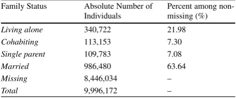
Next, we use the “Family Status” variable to perform an additional check on the validity of our sample. This vari-able is availvari-able as part of the Jobseeker-History ((X)ASU) dataset, and thus is only filled in for a small subset of people – those who are registered as job seekers as of June 30th, 2008.9From our sample of approximately 10 Mio. matched
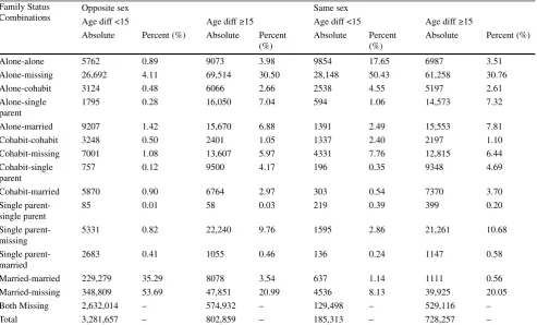
individuals, about 1.5 Mio. have the family status variable filled in. The variable takes on four possible values: living alone, cohabiting, single parent, or married. Table4depicts the distribution of family status values across all individuals with a matched name within their location. Although 85% are missing the family status variable, of those in the data with a family status listed, approximately 64% are listed as married, 22% are listed as living alone, while the rest are ei-ther cohabiting or are single parents. We investigate furei-ther by looking at the combination of family status for matched pairs, shown separately by gender composition and age dif-ference (Table5). When we look at male-female pairs with an age difference under 15 years, we see that, for couples with at least one family status listed, they are listed as ei-ther both married or one married-one missing family status 89% of the time. This is far higher than for same-sex pairs
9 These are typically either people who are unemployed (in
particu-lar unemployment insurance recipients are required to register as job seekers) or who expect to be unemployed soon.
with age difference under 15 years, who are listed as both married or one married-one missing only 9% of the time. Male-female couples with an age difference of 15 years or more are listed as both married or one married-one missing 25% of the time. This could either indicate that there are some married couples with an age difference of larger than 15 years, but could also be because these are indeed parent-child relationships where the spouse is not covered in the data (or does not share a last name).
Using the information in Table 5, we can also estimate the share of matches in our final sample that are likely to be true couples and not wrongly matched people (i. e. our “accuracy rate”) using the subsample of couples with at least one family status listed. If we think that the family status variable is accurate, then the set of “true” couples in our sample should be 578,088: the number of couples who are listed of either being both married or one mar-ried, on missing family status. Even within these there may be individuals who were mistakenly matched. For exam-ple, there may be a job-seeking man with the last name MUELLER, whose wife is out of the workforce (and hence is not included in the IEB data), living at the same coor-dinates as a similarly-aged jobseeker woman with the last name MUELLER whose husband is not in the IEB data ei-ther. Our matching algorithm would connect these two job-seekers, who are both listed as being married, even though they are not actually married to each other. If we think that it is as likely for two individuals of the same gender to be wrongly matched in this way as it is for two oppo-site-gender individuals, then we can use the information on family status for same-sex pairs for our accuracy esti-mate. Specifically, there are 5173 (637 + 4536) same-sex matched pairs with age difference less than 15 years where family status is listed as both married or married-missing.10
Since we know that these are wrongly matched pairs, we can assume that the same number of opposite-sex pairs was wrongly matched as well. So, the estimated “true” number of couples in the subsample of couples with family sta-tus is 572,915 (578,088 matched M-F with age difference <15 and family status married-married or married-missing minus 5173 same-sex pairs with age difference <15 and married-married or married-missing status). Since our full sample of matched couples (with family status) is made up of 649,643 (3,281,657–2,632,014) couples, our estimated accuracy rate is 88.2% (572, 915 “true” couples/649,643 total couples in our final sample of couples with family sta-tus filled in for at least one of the members), or 11.8% error rate.
10 We are again being conservative here, assuming that among the
Table 5 Family Status Composition, for matched couples Family Status
Combinations
Opposite sex Same sex
Age diff <15 Age diff≥15 Age diff <15 Age diff≥15
Absolute Percent (%) Absolute Percent (%)
Absolute Percent (%)
Absolute Percent (%)
Alone-alone 5762 0.89 9073 3.98 9854 17.65 6987 3.51
Alone-missing 26,692 4.11 69,514 30.50 28,148 50.43 61,258 30.76
Alone-cohabit 3124 0.48 6066 2.66 2538 4.55 5197 2.61
Alone-single parent
1795 0.28 16,050 7.04 594 1.06 14,573 7.32
Alone-married 9207 1.42 15,670 6.88 1391 2.49 15,553 7.81
Cohabit-cohabit 3248 0.50 2401 1.05 1337 2.40 2197 1.10
Cohabit-missing 7001 1.08 13,607 5.97 4331 7.76 12,815 6.44
Cohabit-single parent
757 0.12 9500 4.17 196 0.35 9348 4.69
Cohabit-married 5870 0.90 6764 2.97 303 0.54 7370 3.70
Single parent-single parent
85 0.01 58 0.03 219 0.39 399 0.20
Single parent-missing
5331 0.82 22,240 9.76 1595 2.86 21,261 10.68
Single parent-married
2683 0.41 1055 0.46 136 0.24 1147 0.58
Married-married 229,279 35.29 8078 3.54 637 1.14 1111 0.56
Married-missing 348,809 53.69 47,851 20.99 4536 8.13 39,925 20.05
Both Missing 2,632,014 – 574,932 – 129,498 – 529,116 –
Total 3,281,657 – 802,859 – 185,313 – 728,257 –
The sample includes all couples who we were able to match by location and name (according to our name-matching algorithm). Only individuals who are registered as job-seekers have the family status variable filled in
We may expect fewer errors of this type in our matching algorithm if we restrict our focus to coordinates with ex-actly two people – in this case, there are likely to be fewer mismatched pairs of the type described above. When we re-peat the accuracy rate estimation, restricting our sample to matched couples living at coordinates where exactly 2 peo-ple live, we find that to be the case: our estimated error rate is likely a bit lower, around 8.6% (see Appendix Table7).
While using the job-seeker data is helpful for estimat-ing the likely fraction of false positives, it should be kept in mind that neither is this subsample representative, nor necessarily is family status measured without errors. It may well be the case that we are overestimating or underesti-mating the number of false positives here. Overall, based on the two approaches discussed, we estimate that the frac-tion of false positives lies somewhere in the range of 6% to 11.8%.
4.2 Missing couples
Given the data we are using and the matching algorithm we have developed, we are likely to have missed many true married couples, either among individuals who are in our dataset (a form of type 2 error) or where at least one spouse
is not covered in the IEB. In order to get a sense of what share of couples we can identify in our data, we obtained the Scientific Use File of the Microcensus 2008 (see Boehle
2010), to calculate the number of married couples in 2008 overall and the number of married couples that satisfy the sample restrictions that we have to apply in the IEB data. Overall, there were 19,187,000 married couples in 2008; of those, about 9.2 Mio. were such that both spouses would live together, would be less than 15 years apart in age, and would be covered in the IEB data, i. e. either working in a social security covered job or being unemployed. Since, in our final sample, we have 3.2 Mio. couples, we capture about one third of the total number of married couples that match our baseline restrictions.
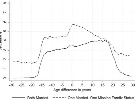
Fig. 5 Share of matched pairs listed as married or married-missing. (Note: Includes all male-female pairs of individuals who we were able to match by location and name (according to our name-matching algorithm), and where at least one member has the family status variable filled in. Age difference is calculated as man’s age – wife’s age)
Couples where the age difference between the husband and wife is more than 15 years are omitted from our sample in an effort to ensure that we do not mistakenly include par-ent-child pairs in our sample. Although there are certainly married couples with a 15-year or larger age difference, the number of these types of couples is quite small. For exam-ple, in the micro census, a representative survey of German households, the share of couples with a 16-year or more age difference was only 2% in 2008.
We also investigated the likely impact of our age restric-tion using the marital status variable available in the job seeker data. For the subsample of couples where we have the marital status for at least one of the two individuals, in Fig.5we plotted the share of couples where either both were reported as married or one person was married and the other person’s marital status was missing. Matched couples where both are married seem to be very rare when the woman is older than 15 years than the man. This suggests that there are almost no true couples that we are missing with the 15 years age difference restriction. On the other end there is still a high share of couples where the man is around 15 to 20 years older than the woman where both are reported as married. If these are true couples, then we are excluding them from our set of likely married couples. No-tice however that while the share is significant, Fig.1shows that there are almost no couples in the 15 to 20 years age window (consistent with the information from the micro census), again suggesting that the 15 years age difference
restriction does not exclude many true couples.11There are
more matched pairs in Fig.1where the man is around 25 years older than the woman, but Fig.5shows that that is ex-actly where the share of married/married is falling to zero, thus suggesting that here we have mainly pairs who are not matched to each other12.
Couples not living together on June 30th, 2008 are im-possible for us to identify with our data; however, we be-lieve that this situation is likely to be rare.
If the couple lives at a location with more than 2 people with the same last name at the same coordinate, we have no way of knowing which two people are part of a couple, and so all are dropped (about 5.2 Mio.).
We drop people who have inconsistent names across data sources, thus potentially omitting more couples from our sample (about 1.8 M).
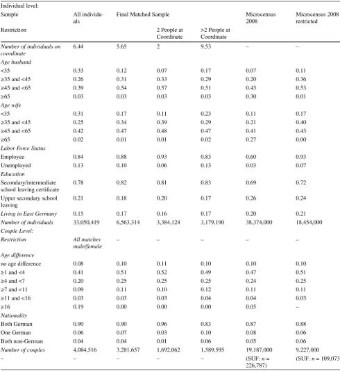
We can get a sense of how representative our final sample of couples is by comparing their characteristics to those of a truly representative sample of couples, those in the Mi-crocensus. Table 6compares individual characteristics of people in our final sample of couples (column 3) to couples in the Microcensus in 2008. Column (6) shows all mar-ried couples in 2008, while column (7) shows all couples satisfying the restrictions of our algorithm in the IEB. In terms of the age distribution, our men and women tend to be a younger than those of all census couples; this can be explained by the fact that our sample only includes people in the workforce, so older workers who are more likely to be retired are excluded. In addition, anyone married to a re-tired person will be omitted from our final sample, since their spouse will not be in our original dataset. Comparing the last column where we apply the same restrictions as in our matching algorithm, we find that the age distribution is much closer to our matched couples.
Looking next at the labor force status, we do not have the full range of labor force status options that are available in the micro census, since the IAB data only includes peo-ple in the labor force but omits self-employed and public servants. The couples in the last column of Table 6 look reasonably similar in terms of labor force status as our matched couples sample, although they are somewhat less likely to be unemployed. This might be because some long-term unemployed who are in the IEB might be identified as out of the labor force in the Microcensus, or because we are somehow more likely to identify unemployed
individ-11 This can also be seen from Table5if we look at the subsample of
our matched couples with the family status variable available. Of the male-female pairs where both are listed as married, only 3% have an age difference of 15 years or more.
12 Appendix Fig.7shows the same figure restricted to couples at
Table 6 Comparing Individuals and Couples with Microcensus Individual level:
Sample All
individu-als
Final Matched Sample Microcensus
2008
Microcensus 2008 restricted
Restriction 2 People at
Coordinate
>2 People at Coordinate
Number of individuals on coordinate
6.44 5.65 2 9.53 – –
Age husband
<35 0.33 0.12 0.07 0.17 0.07 0.11
≥35 and <45 0.26 0.31 0.33 0.29 0.20 0.36
≥45 and <65 0.39 0.54 0.57 0.51 0.43 0.53
≥65 0.03 0.03 0.03 0.03 0.30 0.01
Age wife
<35 0.31 0.17 0.11 0.23 0.11 0.17
≥35 and <45 0.25 0.34 0.39 0.29 0.21 0.40
≥45 and <65 0.42 0.47 0.48 0.47 0.41 0.43
≥65 0.02 0.01 0.01 0.02 0.27 0.00
Labor Force Status
Employee 0.84 0.88 0.93 0.83 0.60 0.93
Unemployed 0.13 0.10 0.06 0.13 0.03 0.07
Education
Secondary/intermediate school leaving certificate
0.78 0.82 0.81 0.83 0.69 0.72
Upper secondary school leaving
0.21 0.18 0.20 0.17 0.26 0.24
Living in East Germany 0.15 0.17 0.16 0.17 0.20 0.21
Number of individuals 33,050,419 6,563,314 3,384,124 3,179,190 38,374,000 18,454,000
Couple Level:
Restriction All matches male/female
– – – – –
Age difference
no age difference 0.08 0.10 0.11 0.10 0.10 0.10
≥1 and <4 0.41 0.51 0.52 0.49 0.47 0.51
≥4 and <7 0.20 0.25 0.25 0.25 0.24 0.25
≥7 and <11 0.09 0.11 0.10 0.12 0.11 0.11
≥11 and <16 0.03 0.03 0.03 0.04 0.04 0.03
≥16 0.19 0.00 0.00 0.00 0.05 –
Nationality
Both German 0.90 0.90 0.96 0.83 0.87 0.88
One German 0.06 0.07 0.03 0.10 0.08 0.06
Both non-German 0.04 0.04 0.01 0.06 0.05 0.06
Number of couples 4,084,516 3,281,657 1,692,062 1,589,595 19,187,000 9,227,000
– – – – – (SUF:n=
226,787)
(SUF:n= 109,073)
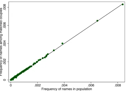
Fig. 6 Frequency of Surnames in Population and Among Matched Couples. (Note: Each dot in the figure represents one unique last name in our data (such as Meier or Mueller). The figure shows the frequency of each last name in the overall population (x-axis) and among the sam-ple of matched cousam-ples (y-axis). The black line represents the 45 degree line, suggesting that most names are equally common in the overall population and among matched couples)
uals as part of couples in the IEB. Interestingly, when we restrict the matched couples data to a sample with exactly 2 people at a location (Column 4) the distribution is much closer to the census.
In the bottom half of Table6we can compare the char-acteristics of couples in the two different data sets. The distribution of age difference within couples of our final sample (column 3) is almost exactly the same as that of the Microcensus when using the same restrictions as in our al-gorithm (column 7). The couples in our sample are slightly more likely to be both German and less likely to be both non-German than those of the micro census; as mentioned earlier, non-Germans are less likely to change their name at marriage than Germans are, and so are more likely to be omitted by our matching algorithm. Overall, although we miss many couples in our data set and may mistakenly in-clude some pairs who are not truly married, the couples that we identify seem roughly similar to the universe of couples in Germany that satisfy the restrictions that are imposed in the matching algorithm.
Finally, we performed an additional check to see whether our algorithm is more likely to pick up very rare or very common last names by comparing the distribution of last names in the overall population with the distribution of last names among matched couples. On the one hand, we might be more likely to find unique matches in the case of rare last names, in which case rare last names would be more common in our matched couples data than in the overall population. On the other hand we might be more likely to obtain false positives in the case of common last names, in which case those would be overrepresented in our matched data. Fig.6shows a scatterplot, where each dot corresponds
to a single last name, relating the frequency of that name in the overall population (on the x-axis) with the frequency of that name among matched couples (y-axis). The black line represents the 45 degree line. Amazingly almost all names are very close to the 45 degree line, suggesting that neither very rare nor very common last names are more or less likely to be matched. Again, while we are clearly not obtaining a representative sample, it is interesting that we do not seem to be biased against particularly common or rare last names.
5 Discussion and conclusion
We present a new method for identifying a very large num-ber of pairs of individuals who are likely married to each other in the German administrative data. While room for type 1 (false positives) and type 2 (false negatives) errors exists, our analysis suggests that our final sample still con-tains about 89 to 94% actually married couples. An im-portant caveat is that due to the nature of the IEB, our sample of married couples is not representative of all mar-ried couples, but at best representative of couples where both individuals are either working in a job that is cov-ered by social security (that is not civil service job or self employed) or are unemployed and receiving benefits. Our comparison with the Microcensus from our baseline year suggests that our matched couples look reasonably similar to couples in this more restrictive sample frame, but even then we are more likely to pick up married couples who live in smaller buildings, such as single family homes, and thus probably couples who are either living in less densely pop-ulated areas or with higher income levels. Finally, since we rely on last names our sample will miss all couples where the spouses do not share a name and this decision is likely correlated with other characteristics of the couple.
While the representativeness of this matched couple data is therefore clearly limited, many research questions do not rely on a representative sample. Most natural experiments that have been used by applied researchers only affect a very selected subsample of the population (e. g. typical regres-sion discontinuity or regresregres-sion kink designs), but obtaining causally interpretable parameters with a high degree of in-ternal validity is still very valuable even if it cannot easily be extrapolated to the general population.
stud-ied the added worker effect, which is whether spouses of displaced workers respond to the job loss by increasing their own labor supply (see for example Lundberg1985, or Stephen2002). Most existing work in this literature has relied on panel survey datasets such as the PSID or GSOEP. Using our identifier, it will be possible to study the added worker effect for a much larger sample of workers after a variety of well identified shocks such as plant closings or mass layoffs. Another promising area of research is to study spillover effects of public programs. For example, Cullen and Gruber (2000) provide fascinating evidence that more generous unemployment insurance benefits reduce la-bor supply of spouses married to the benefit recipient. A lot of recent work on UI has been done with the German admin-istrative data (e. g. Schmieder et al.2012,2016) exploiting the large number of observations and clean sources of iden-tification such as age discontinuities in potential duration. With the possibility to link married couples it will be pos-sible to use similar research designs to look at questions as in Cullen and Gruber (2000) to understand how households as a whole are affected by policies such as UI, active la-bor market policies or tax policies. Another example where
Table 7 Family Status Composition, for matched couples living at coordinates with exactly 2 people total
Different sex Same sex
Age diff <15 Age diff≥15 Age diff <15 Age diff≥15
Combinations Absolute Percent (%)
Absolute Percent (%)
Absolute Percent (%)
Absolute Percent (%)
Alone-alone 1228 0.54 1504 2.08 2385 14.38 1278 2.01
Alone-missing 9956 4.42 30,437 41.99 10,765 64.92 27,634 43.44
Alone-cohabit 412 0.18 624 0.86 338 2.04 542 0.85
Alone-single parent
293 0.13 1922 2.65 95 0.57 1864 2.93
Alone-married 1170 0.52 4106 5.67 280 1.69 3840 6.04
Cohabit-cohabit 431 0.19 226 0.31 132 0.80 213 0.33
Cohabit-miss-ing
1742 0.77 3622 5.00 903 5.45 3537 5.56
Cohabit-single parent
98 0.04 1103 1.52 13 0.08 1136 1.79
Cohabit-mar-ried
915 0.41 1118 1.54 39 0.24 1122 1.76
Single parent-single parent
22 0.01 8 0.01 15 0.09 40 0.06
Single parent-missing
1595 0.71 4420 6.10 339 2.04 4154 6.53
Single parent-married
357 0.16 212 0.29 11 0.07 223 0.35
Married-mar-ried
47,922 21.25 1404 1.94 77 0.46 211 0.33
Married-miss-ing
159,344 70.67 21,774 30.04 1190 7.18 17,816 28.01
Both missing 1,466,577 – 326,445 – 67,477 – 302,644 –
Total 1,692,062 – 398,925 – 84,059 – 366,254 –
Includes all couples who we were able to match by location and name (according to our name-matching algorithm), restricted to couples living at coordinates where no other people are listed. Only individuals who are registered as job-seekers have the family status variable filled in
our new identifier could be used is to study relative in-comes within married couples as for example in Bertrand et al. (2015). Other areas where important work has been done with the IAB data that could be extended using our couple identifiers include for example the labor supply and mobility responses to immigration shocks (Dustmann et al.
2016), or the effects of maternity leave policies on labor supply (Schönberg and Ludsteck2014).
We believe that providing access to a new way to study household decisions and responses in administrative data will inspire the research community to many new and cre-ative research projects.
Open Access This article is distributed under the terms of the Creative Commons Attribution 4.0 International License (http:// creativecommons.org/licenses/by/4.0/), which permits unrestricted use, distribution, and reproduction in any medium, provided you give appropriate credit to the original author(s) and the source, provide a link to the Creative Commons license, and indicate if changes were made.
Fig. 7 Share of matched pairs listed as married or married-missing; 2 people at a coordinate. (Note: Includes all male-female pairs of individuals who we were able to match by location and name (ac-cording to our name-matching algorithm), and where at least one mem-ber has the family status variable filled in. Restricted to couples living at coordinates where exactly 2 people are located. Age difference is calculated as man’s age – wife’s age)
References
All-in: Immer mehr behalten ihren Geburtsnamen – Zahl der Ehen mit Doppelnamen bleibt seit Jahren gleich (2006).http://www. all-in.de/nachrichten/lokales/Immer-mehr-behalten-ihren-Geburtsnamen;art26090,215128, Accessed September 1, 2014 Bertrand, M., Kamenica, E., Pan, J.: Gender identity and relative
in-come within households. Q J Econ130(2), 571–614 (2015) Boehle, M., Schimpl-Neimanns, B.: GESIS – Leibniz-Institut für
Sozialwissenschaften (Ed.): Mikrozensus Scientific Use File 2008 : Dokumentation und Datenaufbereitung. Bonn (GESIS-Technical Reports 2010/13) (2010).http://nbn-resolving.de/urn: nbn:de:0168-ssoar-207237
Cullen, J.B., Gruber, J.: Does unemployment insurance crowd out spousal labor supply? J Labor Econ18(3), 546–572 (2000) Dustmann, C., Schönberg, U., Stuhler, J.: Labor supply shocks, native
wages, and the adjustment of local employment. Quarterly Journal of Economics 132 (1), 435–483 (2017)
Frimmel, W., Halla, M., Winter-Ebmer, R.: Can pro-marriage policies work? An analysis of marginal marriages. Demography 51(4), 1357–1379 (2014)
Goldschmidt, D., Schmieder, J.F.: The rise of domestic outsourcing and the evolution of the German wage structure, Quarterly Journal of Economics (forthcoming)
Hardoy, I., Schøne, P.: Displacement and household adaptation: In-sured by the spouse or the state? J Popul Econ27(3), 683–703 (2014)
Hethey-Maier, T., Schmieder, J.F.: Does the use of worker flows im-prove the analysis of establishment turnover? Evidence from Ger-man administrative data. J Appl Soc Sci Stud – Schmollers Jahrb 2013133(4), 477–510 (2013)
Huttunen, K., Kellokumpu, J.: The effect of job displacement on cou-ples’ fertility decisions. J Labor Econ34(2), 403–442 (2016) Jacobson, L.S., LaLonde, R.J., Sullivan, D.G.: Earnings losses of
dis-placed workers. Am Econ Rev83, No. 4, 685–709 (1993) Janisch, W.: Namenswahl nach der Heirat: Bekenntnis zum Mann
(2010). http://www.sueddeutsche.de/leben/namenswahl-nach-der-heirat-bekenntnis-zum-mann-1.79245, Accessed August 1, 2016
Kammergericht Berlin: Eheregistereintragung: Schreibweise von Ehenamen und Begleitnamen (2013).http://www. gerichtsentscheidungen.berlin-brandenburg.de/jportal/? quelle=jlink&docid=KORE209412013&psml=sammlung.psml& max=true&bs=10, Accessed September 1, 2014
Lundberg, S.: The added worker effect. J Labor Econ3, 11–37 (1985) Schild, C.-J., Antoni, M.: Linking survey data with administrative so-cial security data – the project “Interactions between capabilities in work and private life”. Working paper series, vol. 2014–02. German Record-Linkage Center, Nürnberg, p 11 (2014) Schmieder, J.F., von Wachter, T., Bender, S.: The effects of extended
unemployment insurance over the business cycle: Evidence from regression discontinuity estimates over 20 years. Q J Econ127(2), 701–752 (2012)
Schmieder, J.F., von Wachter, T., Bender, S.: The effect of unemploy-ment benefits and nonemployunemploy-ment durations on wages. Am Econ Rev106(3), 739–777 (2016)
Scholz, T., Rauscher, C., Reiher, J., Bachteler, T.: Geocoding of Ger-man administrative data. FDZ-Methodenreport, vol. 2012–09. In-stitute for Employment Research, Nürnberg, (2012)
Schönberg, U., Ludsteck, J.: Expansions in maternity leave coverage and mothers’ labor market outcomes after childbirth. J Labor Econ32(3), 469–505 (2014)
Sperling, F.: Familiennamensrecht in Deutschland und Frankreich: eine Untersuchung der Rechtslage sowie namensrechtlicher Kon-flikte in grenzüberschreitenden Sachverhalten. Mohr Siebeck, Tübingen, p 226 (2012)
Statistisches Bundesamt: Bevölkerung und Erwerbstätigkeit – Haushalte und Familien Ergebnisse des Mikrozensus, 1st edn. 3. Statistis-ches Bundesamt, Wiesbaden (2012)
Stephens Jr, M.: Worker displacement and the added worker effect. J Labor Econ20(3), 504–537 (2002)
Deborah Goldschmidt Associate, Analysis Group
Wolfram Klosterhuber Research Fellow, Institute for Employment Research (IAB)