Towards shortest path identification
on large networks
Haysam Selim
*and Justin Zhan
Introduction
Over the past 10 years, there has been vast improvement in hardware architecture design for computer information, one of the most important functions being network analysis. The main problem with network analysis is the shortest path analysis. Accord-ing to the network beAccord-ing analyzed, the shortest path has a variety of measurements, such as time, to find the path. The problem with determining the shortest path, however, is to find both the fastest and the shortest path. Thus, research in the shortest path always has been a point of interest in graph theory.
Frequently, graphs are used along with modern technology in such setting as online social networks (e.g., LinkedIn™ or Facebook). Since the size of the graphs is increasing exponentially, many direct processes become more demanding. For example, LinkedIn— a well-known website for professional networking—that tries to connect professionals together worldwide. If a person is trying to get in touch with someone from the human resource department in a company by using LinkedIn, what the website does is try to find the shortest path to reach that person in that specific company, starting from his connections and moving on to friends of friend to reach the desired personal in the specified company. Similarly, this application of the shortest path can be used over and over in different scenarios, for example, finding routes from one point to another point
Abstract
The use of Big Data in today’s world has become a necessity due to the massive num-ber of technologies developed recently that keeps on providing us with data such as sensors, surveillance system and even smart phones and smart wearable devices they all tend to produce a lot of information that need to be analyzed and studied in details to provide us with some insight to what these data represent. In this paper we focus on the application of the techniques of data reduction based on data nodes in large net-works datasets by computing data similarity computation, maximum similarity clique (MSC) and then finding the shortest path in a quick manner due to the data reduction in the graph. As the number of vertices and edges tend to increase on large networks the aim of this article is to make the reduction of the network that will cause an impact on calculating the shortest path for a faster analysis in a shortest time.
Keywords: Network, Network analysis, Similarity graph reduction, Shortest path analysis, Dijkstra’s, Maximum similarity clique (MSC), Data similarity computation
Open Access
© 2016 The Author(s). This article is distributed under the terms of the Creative Commons Attribution 4.0 International License (http://creativecommons.org/licenses/by/4.0/), which permits unrestricted use, distribution, and reproduction in any medium, provided you give appropriate credit to the original author(s) and the source, provide a link to the Creative Commons license, and indicate if changes were made.
RESEARCH
in GPS navigation system. In many cases, when finding the shortest path, in a selected graph that consists of millions of nodes and edges the measurability and accuracy becomes more complex to measure, the shortest path query must respond to the request as fast as possible with high accuracy. Although the graph may comprise of a lot of nodes and edges but the shortest path must be calculated fast, as an example in car navigation (GPS) an alternative route could be used [1] to provide the driver with a driving route to the requested destination in a given situation the driver would prefer a quick response that is accurate to make right decisions while driving thus a much faster response time is a necessity in this case.
Background
Computing the path in cluttered environments that contain a lot of nodes and with millions of vertices where some vertices might be fairly similar or relatively close still consumes a lot from the computation prospective and makes computation much more complex. The desire to produce algorithms that are complete, i.e., algorithms that find a path if one exists—have resulted in computationally impractical when applied to high dimensionality problems despite their relatively low (polynomial) complexity. It is essen-tial to address practical motion-planning problems in complex industrial environments as discussed that led to the development of probabilistic and Monte Carlo search algo-rithms, typically known as the random roadmap approach [2]. While the probabilistic algorithms effectively trade-off completeness for computational efficiency, they have difficulties in finding valid paths through narrow corridors in the free space, where the probability of sampling configurations is low.
The computation cost to compute the path using an approach, such as the algorithm proposed by Fujita et al. [2] or other similar approaches [3–6] such as Dual Dijkstra’s Search (DDS) were unlike randomized algorithms, it searches over the entire configu-ration space to simultaneously generate the global optimal path, in addition to several distinct local minima. The procedural part of this approach is to run the Dijkstra’s search twice so that it produces a list of ranked paths that span the entire graph in order of opti-mality. There have been numerous ways that helps to calculate the shortest path by using several techniques as the one proposed in [2] and they work perfectly but they have a high cost of computation specially when the number of nodes increases. The computa-tion of typical algorithms for K-best paths [7, 8] is linear in the number of paths (K), that may be enormous if the paths are to span throw the entire graph. In contrast, the Dual Dijkstra’s Search computes paths that span the entire graph at a computational cost that is independent of the number of paths generated. The DDS requires two Dijkstra’s searches, similar to K = 2 [2].
The approaches were Dijkstra’s search that computes the shortest paths from the start node to all other nodes in the graph. For every node, it computes and stores the mini-mum cost to the start node and the previous node on the optimal path. By tracing back to the previous node, it is possible to generate the optimal path. This algorithm is useful for generating only the optimal path between any two nodes, and cannot generate other candidates paths between the two nodes [2].
pass through that node. In the second step, the shortest path is selected in each homot-opy class [9].
Typical algorithms for computing the K shortest paths [7, 8] first search for the opti-mal path, then search for the second best, the third, and so on. This approach has several disadvantages:
1. The computational cost grows linearly with K.
2. Paths are found in a decreasing order of optimality, generating many ‘similar’ paths.
Another reason why best-first search (BFS) doesn’t work for weighted graphs as there could no longer an assurance that the node at the top of the queue is the node that is the closest or nearest to s. It is certainly the closest in terms of the number of edges used to reach it, but not in terms of the sum of edge weights. Although this issue could be fixed instead of using a plain queue, a priority queue can be used, in which vertices are sorted by their increasing dist[] value. Then, at each iteration, select the node x, with smallest dist[x] value and call relax (x, y) on all of its neighbors, y.
This evidence of exactness is typically the same towards BFS, and the same loop invari-ant holds. However, this algorithm approach works only as long as there are no edges that has a negative weight. Or else there is no assurance that when x is selected as the nearest node, dist[y] for some other vertex y will not become smaller than dist[x] at a point upcoming.
There are several ways to implement Dijkstra’s algorithm. One of the main challenges that’s to support a priority queue of vertices that offers three main processes: Adding new nodes to the queue, removing the nodes with smallest dist[], and reducing the dist[] value of some nodes during relaxation [10]. A set can be used to represent the queue. This approach of implementation will look similar to the BFS.
Shortest distances have been used as an underlying metric in a number of measures, such as centrality. One of these measures is betweenness, which is equal to the number of shortest paths between others that pass through a node.
The Dijkstra’s algorithm selects a source node and loads in the dist[] array with the shortest path distances from s. All the distances that are initialized to infinity, except for dist[s], which are set to 0. Then, s is added to the queue, and the same process continues as for BFS: remove the first node x, and scan all of its neighboring node, y. Then the new distance to y is computed, and if it is better than the currently known distance, it is updated [11].
Problem definition
is important as it shows how it would perform as the input size grows [12]. Dijkstra’s method is one of the well-known algorithms, and that have been used and implemented in several applications and in several approaches.
In this study, a benchmark dataset was tested from UNC The Odum Institue, [13–15] Where we used the data source from there Dataverse Network, the input dataset consists of a collection of XML files Extensible Markup Language, using the standard implementa-tion and just trying to run such dataset or even larger set of data affects the running time as well as might affect the decision making process in case of a real-time necessity. Due to several computation nodes that maybe irrelevant. As a result of this delay in responding which might not be acceptable in some programs or some other cases. The main reason for this delay in Dijkstra’s algorithm is that it has to build and keep the shortest path to all nodes in the graph whose distance to the source or main node is less than the distance from the source node to the final node or the destination node. Thus in such a case the consumption of memory by this classical algorithm “Dijkstra’s algorithm” is excessive and too demanding to maintain a large amount in the memory as it’s a large network that con-sist of millions of nodes it’s absurd and costly for parallel execution of all these queries.
Definition 1 In a weighted directed graph G = (V, E), an edge is adjacent to an edge
Vj, Vk is adjacent to an edge Vi, Vj if and only if Vi, Vjʹ Vk ∈ V, Vi, vj and vj, vk ∈ E.
Definition 2 (Direct adjacent edges/indirect adjacent edges) If there is no cost from an edge to its adjacent edge, the adjacent edge is called the edge’s direct adjacent edge. Oth-erwise, it’s called the edge’s indirect adjacent edge. The weight of an indirect adjacent edge represents the cost from an edge to its adjacent edge.
Definition 3 Line In a weighted directed graph G = (V, E), a line from vp to vq is the vertex sequence vp = ViO, ViI,…,vm = vq, where �Vij−1� vu, and �Vij, Vij+1� ∈ E and an edge �Vij, Vij+1� is the direct adjacent edge of an edge �vij−1, vij� (1 ≤ j ≤ m − 1).
The method used in this paper uses Dijkstra’s algorithm that marks the start point in a network and then it calculates the cost of moving from the start node to each node and marks the node with the least value. Then it repeats this process this step several times until the destination is marked and reached.
To modify this algorithm to work in a specified time by making the algorithm run in both directions that beans that the algorithm starts from the beginning node and starts to calculate the cost of each value of each movement to each node while at the same time starts at the end node to do the same calculation but starting from the last node this time and calculating the cost to each node. Yet this method has a major disadvantage [16] that is by using this method to obtain a result these results could not be obtained in a real-time situation.
Our approach
that starts with an initial node and ends with one final node. Which means that these initial nodes have no incoming edges connected to it and the final node doesn’t have any outgoing edges of it. The hassle with these directed graphs is that it has structural con-flicts like deadlocks and lack of synchronization [20] may occur if the workflow graph wasn’t designed correctly.
In such cases of large network and where an ideal and a quick response is required it’s preferably as an initial step for us to do is to aim for a graph reduction. Where trying to reduce large amount of data depending on many certain methodologies that are based on Similarity graph reduction (SGR) [21, 22] that will help in solving the main aim that is reducing a graph to a simple structure that will help us to reveal some information that were previously difficult to be discovered or it took a lot of time to figure out this information. Thus we will be reducing the graph on similarity bases and by computing similarity that gives us a final reduction graph. This graph will be based on a certain threshold [23, 24] after reducing our large graph by applying the reduction algorithm.
The use of the shortest path algorithm is a commonly used nowadays and can be seen in a lot of common applications that we use in our daily life as an example the Naviga-tion systems [1]. This made me more interested to research on this topic as improving the response time that is given to us from this algorithm could lead into a lot of better improvements and better decision in a smaller time frame making faster decisions more reliable and in certain cases giving a better response time to the tool where this algo-rithm will be used, especially if the path consist of a lot of data (nodes, edges) and a lot of alternative paths thus making it take much longer to find the shortest path. Therefore this algorithm has a lot of use and as well a lot of benefit, this made me more motivated to work on this topic.
In this section of the paper we talk about the procedure and the Algorithm used and the steps made to make the reduction and then finding the shortest path after the reduc-tion part has been made.
Network reduction
In the reduction graph that is based on similarity the main aim is to gain a less complex (similarity) graph through the given original graph. As the Author [23] in this paper he defined the SGR were the formal definition he defines is as follows:
Definition 4 [Similarity graph reduction (SGR)] Given an similarity graph, G = (V, E), the goal of SGR is to generate a Gʹ = (Vʹ, Eʹ) such that it suffices |Vʹ| < |V| and |Eʹ| < |E|.
As shown from the definition of the author [22] that if a similarity value of a couple of nodes is adequately high then we can assume that the distance between both the nodes is negligible. Thus let’s assume two nodes that are identical have a similarity value being 1 hence their distance will be assumed as 0 this represents a complete overlapping graph. Therefore the author introduces another definition that will help in proceeding without loss in generality.
forms a complete similarity graph; (2) The similarity value on each pair of the edges of the complete graph is sufficiently large, such that S (u, v) ≥ θ where u, v ∈ N and u ≠ v.
This section of reduction aims to find a similarity clique [22] for situations that has more than two nodes it does so by presenting an arbitrary threshold value θ. The thresh-old value will assist in controlling the SC’s similarity level through adjusting the value of θ. The similarity clique collects groups of nodes that have negligible distances. Thus for the aim of reduction we need the maximal similarity clique (MSC) that’s defined as the following:
Definition 6 [Maximal similarity clique (MSC)] A similarity clique is said to be a max-imal similarity clique if it violates the necessary and sufficient conditions of being a simi-larity clique by adding one more adjacent vertex.
Then from this result we try to combine the entire maximal similarity clique [22] into a single node thus making the number of nodes and as well as the number of edges in the graph to be reduced. As the author in paper [22] explained the main reason for this reduc-tion is because with every k-node maximal similarity clique its replaced with a single node where there is at least k2−k
2 edges and a k − 1 nodes reduced from the original graph.
Shortest path
Shortest path on large graphs might not be an easy task as there are a lot of nodes and alternatives in that graph thus it takes a lot of time and as well as computational efforts to find the shortest path [1, 6]. By using Dijkstra’s algorithm to calculate the shortest path between two nodes in a graph has the asymptotic runtime complexity of O (m + nlog (n)), where n is the number of nodes and m is the number of edges. We will insert the network graph that will be used in Dijkstra’s method it will use the reduced graph from SGR the method we used before thus reducing the size of the graph and will help in giv-ing a better upgrade in performance wise in Dijkstra’s method.
Principle of dijkstra’s shortest path
The main hypothesis of this algorithm works the following way:
• Select the source vertex.
• Define a set N of nodes; Initialize it to an empty set or infinite. Along the Algorithm and as it moves along these set N will be updated with those nodes that the shortest path has found.
• Start the source Node with 0, and then insert it into N.
• Then we consider each node not in N that it’s connected by an edge from the newly inserted Node. Label the node not in N with the label that’s inserted newly into the node and add the length of the edge. (If the node is not in N its new label will be the minimum)
• Select the vertex that’s not in N with the least label and add it to N.
Thus if the final destination that is required is labeled, then its label will be the distance from the source till the destination. If it isn’t labeled, thus we can assume that there isn’t a path from the source to the destination required.
As shown in Fig. 1 an undirected graph network that’s weighted to clarify the proce-dure from this sample graph we are able to create the adjacency matrix and a distance matrix as well by creating a square matrix of size N × N (di j).
The matrices will be created from the input data and visualized as shown in Fig. 1 where these matrices helps also in the process of analysis of the graph either it’s a social network graph that represents people and their communication with each other, friend connection on social network or even flight records analysis or all flights from one air-port to another these helps us to have a better understanding and a better means for structural analysis and visualization techniques such as the work presented in [11, 25, 26]. Complex large scale networks are massive in size of data and the information that they hold and contain. Analysis and the interactivity of a network and in particularly network that deal with large scale “Big Data” have vital importance. As our networks are evolving incessantly and constantly tools that are used must be scalable and must main-tain a superior visualization and interactivity as visualization plays an important role in understanding the big picture of the network as well as reveals to us hidden factors that weren’t made clear before therefore these methods are a necessity.
As shown in Fig. 2a and in Fig. 2b the matrices of the graph in Fig. 1 created where in Fig. 2a the matrices represent 0’s and 1’s where 0’s represents no edges between certain nodes and 1’s
Fig. 1 Sample undirected weighted graph
represent a weighted edge available between these nodes. As for the matrix in Fig. 2b repre-sent the distance matrix for the graph for calculation of the path where it updates the matrix with each loop as explained later in the algorithm section of this paper, after the updating the distance matrix the measures or the weights of distance in the graph are important indicators in the process of statistical analysis. It quantifies dissimilarity between sample data for numer-ical computation. These distance methods data using a matrix of pairwise distances.
Inserting the weights to the matrix in Fig. 2a yields the distance matrix that makes it easier to calculate many analysis functions that are important such as clustering coef-ficient, degree distribution, the distance matrix created in Fig. 3 is an appropriate way to represent the dataset and make it much more uncomplicated and simpler to analyze the dataset and to visualize it. Splaying the dataset onto an adjacency matrix helps to display the graph and gather all the information that the dataset would have and thus can be represented in a more efficient way.
In Fig. 4 we use the same network graph used in Fig. 1 to show how the steps are cov-ered during analysis of the graph to calculate the path between nodes. As shown in Fig. 4 we use node A as the start node and set the final destination as node F in the second step we calculate the lowest cost to reach the next node from node A and so on. As explained in the figure relating to the algorithm stages Figs. 1–4 expressed the phases from the start node A followed by node C then to node D and finally to the selected destination F traversing through the start node to the destination in the shortest possible path.
Fig. 3 Distance matrix
Algorithms
The similarity value is usually normalized in the domain of [0, 1], with a value of 1 indi-cating identical and a value of 0 implying completely different [22]. As an adjacency matrix, the data structure that stores an undirected graph, a similarity adjacency matrix is the data structure that stores a similarity graph and as long as a similarity adjacency matrix is filled out, the relevant similarity graph then can be plotted.
To explain the process of similarity value computation, the data points, X = {X1, X2,…,Xn} and Y = {Y1, Y2,…,Yn}. ∀ Xk ∈ X and ∀Yk ∈ Y, |Xk| = |{x1, x2,…, xi}| = ik and |Yk| = |{y1, y2,…, yj}| = jk. This indicates that both categorical attributes, Xk and Yk, have a number of ik and jk values [22]. The method of similarity computation for two data points is described in algorithm 1. The algorithm requires two data points as its input and outputs a similarity value. Specifically, for each attribute of X and Y, the algorithm first stores a smaller attribute cardinality to K, then it computes an attribute similarity matrix. All elements in the matrix are then extracted into a value list. The value list is sorted such that the mean of the top K values can be computed and assigned as Sk(Xk, Yk). At last, S(Xk, Yk) can be obtained through a weighted sum of each Sk(Xk, Yk).
The new cliques algorithm (Algorithm 3) above [22] describes the process of producing a list of new cliques [22], in which the new cliques do not contain any repeating vertex. The algo-rithm first compares each clique in the input list to identify if there are any repeating vertices. If there do exist repeating vertices, the algorithm returns the input clique list; otherwise, it first compares similarities for each pair of cliques listed in Cliques and merges repeating nodes into the clique having maximum similarities and then it removes cliques with only one node left and returns a list of new cliques. The reduced graph consists of a list of vertices Vʹ, Where Vʹ = V\VNewCliques ∪ {m}. Where if we Let V1 = V\VNewCliques, V2 = {m}. Thus, all similarity edges of the graph forms a set of E, where E ⊆ {V1 × V1} ∪ {V1 × V2}∪{V2 × V2}. Edges in V1 × V1 can be directly inherited from E, the original edge set, since the similarity value of each edge remains the same. However, for the edges in V1 × V2 and V2 × V2, the computation of similarity values is required because of the m new nodes
The new cliques algorithm (Algorithm 3) above [22] describes the process of producing a list of new cliques [22], in which the new cliques do not contain any repeating vertex. The algo-rithm first compares each clique in the input list to identify if there are any repeating vertices. If there do exist repeating vertices, the algorithm returns the input clique list; otherwise, it first compares similarities for each pair of cliques listed in Cliques and merges repeating nodes into the clique having maximum similarities and then it removes cliques with only one node left and returns a list of new cliques. The reduced graph consists of a list of vertices Vʹ, Where Vʹ = V\VNewCliques ∪ {m}. Where if we Let V1 = V\VNewCliques, V2 = {m}. Thus, all similarity edges of the graph forms a set of E, where E ⊆ {V1 × V1} ∪ {V1 × V2}∪{V2 × V2}. Edges in V1 × V1 can be directly inherited from E, the original edge set, since the similarity value of each edge remains the same. However, for the edges in V1 × V2 and V2 × V2, the computation of similarity values is required because of the m new nodes
A New Cliques list with m cliques forms m new vertices for the reduced similarity graph [22].
The algorithm has two sets of nodes that are maintained that are as follows:
the weight of the value is less than that’s what is unavailable and we repeat this step till all nodes are available in E.
Then the similarity graph reduction algorithm [22] reduces the total number of verti-ces within a similarity graph that merges every vertex involving in a maximal similarity clique into one node.
Experiment
The Objective of this experimentation is to input a graph data and successfully imple-ment reduction on the graph then computing the path based on the reduced graph that’s based on the similarity clique process. The Dataset collected to run on this experiment was from UNC The Odum Institue, [13–15] Where we used the data source from there Dataverse Network, the input dataset consists of a collection of XML files. This Research has been tested and conducted on a Lenovo Y510P with 4th Generation Intel® core i7- 4700MQ processor with a 2.4 GHz 1600 MHz, 8 GB of (RAM) with Graphics NVIDIA® GeForce® GT755 M 2 GB. This paper introduces a concept of finding the shortest path in a large undirected Network graph by using a reduction algorithm to reduce the size and this will have a large impact on the performance. This proposed algorithm makes use of the similarity Clique “SC” and the maximum similarity clique “MSC” developed by our colleague and published in [22] to make the reduction effective. This algorithm is applied to the network with huge nodes to support the network analysis process that we developed [11, 25, 26].
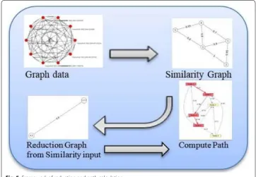
Figure 5 illustrates the frame work followed to shed light on the procedure followed after the collection of the data from Dataverse in XML format its then preprocessed to form the graph data network based on interactions and weight is represented as edges between nodes. Then the process of calculating similarities in graph based on the
definitions and algorithms discussed on the previous section to output the reduction graph the similarity is also based on a threshold set to form the cliques then based on this reduction graph on a large network a path could be determined from this reduced graph.
After the similarity graph reduction process have been applied to a large graph the algorithm starts working as explained in the previous section by finding similarities and then applying the maximum similarity cliques to the graph by grouping nodes that are connected through similarity edges and then followed by the similarity graph reduction that reduces the graph G, after this process has been done the simulation time on the reduced graph becomes much faster since the graph has been reduced using the algo-rithm proposed, Then the process of calculating the shortest path in the reduced graph starts using Shortest path calculation algorithm. This greedy algorithm has a complexity of O (m) where m represents the number of edges in a given graph.
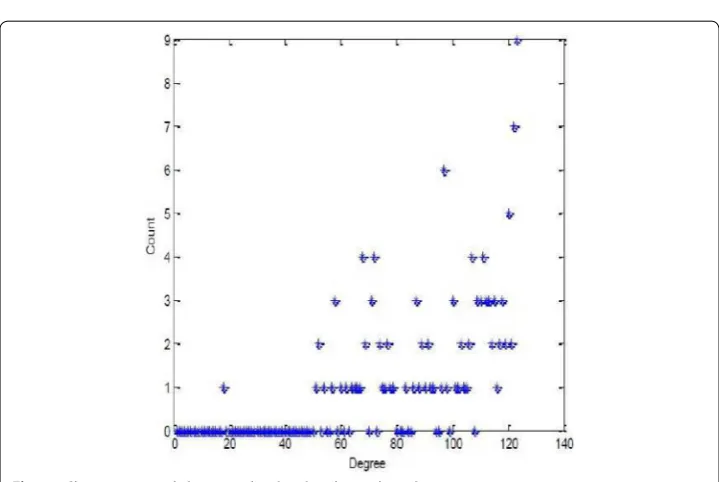
As represented in the framework of the reduction Fig. 5 and path calculation Fig. 4, on the procedure and the flow between algorithm stages on the graph data using MSC algorithm (Algorithm 2), then forming new cliques using New Cliques Algorithm 3 and Similarity Graph Reduction Algorithm 4 to effectively reduce the size of the graph effec-tively where as in Fig. 6 where it represents the graph data before reduction as in nodes and edges and Fig. 7 represents the same data but after applying the reduction where the number of edges have decreased and Figs. 8 and 9 similarity clique process while adjust-ing the threshold applied regardadjust-ing the edges usadjust-ing this data to find the shortest path by using the path Calculation Algorithm. After this process of reduction and the graph have been reduced we apply the path calculation algorithm to calculate the distance based on the weights of the edges on the reduced graph. Figures 10 and 11 represents count of edges or degrees in two graphs Erdos Collaboration network and Slovenian journal that is a weighted undirected graph.
To further more clarify this method of reduction on the network we demonstrate a sample small network in Figs. 12 and 13 that consist of five nodes, where we are given a similarity graph to show the procedure of the process as follows:
Fig. 7 Graph reduction similarity clique process
Fig. 8 Similarity clique process
• Calculate and do the maximum similarity clique giving us {1, 2, 3} and {3, 4, 5} based on the set threshold that’s set to 0.8 in this sample.
• Remove the repeating vertex 3 from the clique {3, 4, 5}, since the clique {1, 2, 3} takes more similarities than the other one.
• forms a new edge between the two new nodes, where the similarity value is com-puted as S(1,4)+S(3,4)+S(3,5)
3 = 0.8.
Fig. 10 An analysis on a network graph degrees on Erdos collaboration network
Figures 12 and 13 demonstrate the reduction from 5 nodes to 2 nodes while retaining the information of other nodes that where combined [22].
Conclusion
We have proposed in this paper a fast method and an algorithm for the approximation and reduction of a large network and a fast estimate calculation for the shortest path, in addition to previously proposed algorithms for distance estimation. We described an uncomplicated yet powerful approach to the graph data that will function on the col-lected similarity graph data that is computed by the reduction algorithm and achiev-ing at query execution time that beat’s up the classical Dijkstra’s shortest path algorithm with large datasets. Thus this will help some other application that uses a large network to have a better, faster response time further experiments could be done using alterna-tive data reduction methods that might have an effect on data reduction with greater
Fig. 12 Similarity graph
response time. Along with the rise of Big Data and vast increase in volumes and the diversity of the data.
This vast increase in the volume and also the diversity (variety) of the data as well as the speed or velocity that these data are generated with along with the veracity, uncer-tainty of the data due to certain inconsistency or the ambiguity generated from such data makes it a Big Data problem by covering the main four characteristics of Big Data (vol-ume, velocity, variety, veracity).
Another further method that could be implemented is by modifying the algorithm in finding the shortest path to try to eliminate the 0 or infinite values. Thus reducing the load on the memory and could result in a faster response.
This approach has helped by reducing the number of edges in a network graph and as well as nodes in the graph by combining similar nodes based on the MSC algorithm. Authors’ contributions
HS performed the primary literature review, data collection, experiments, and also drafted the manuscript. JZ worked with HS to develop the algorithm, articles and the framework. All authors read and approved the final manuscript. Authors’ information
Haysam Selim is a Ph.D. Student at the Department of Computer Science, University of Nevada, Las Vegas (UNLV). His research interests include social computing, machine learning, and Graph Theory. Mr. Selim holds one Master’s degree in computer science from North Carolina A&T State University, and one Baccalaureate degree in Information Technology in Network Security from American University in the Emirates (AUE), Dubai, United Arab Emirates (U.A.E).
Dr. Justin Zhan is an associate professor at the Department of Computer Science, University of Nevada, Las Vegas (UNLV). He previously been an associate professor at the Department of Computer Science North Carolina A&T State University. He has been a faculty member at Carnegie Mellon University and National Center for the Protection of Financial Infrastructure in Dakota State University. His research interests include Big Data, Information Assurance, Social Computing, and Health Science.
Acknowledgements
We are thankful to The United States Department of Defense (DoD Grants #W911 NF-13-1- 0130), National Science Foundation (NSF Grant #1560625), and Oak Ridge National Laboratory (ORNL Contract #4000144962) for their support and finance for this project. This work is supported by The United States Department of Defense (DoD Grants #W911 NF-13-1- 0130).
Competing interests
The authors declare that they have no competing interests.
Received: 21 February 2016 Accepted: 12 May 2016
References
1. Palmer C, Cragin M, Smith L, Heidorn P. Data curation for the long tail of science: the case of environmental science. In: Third international digital curation conference, Washington, DC. 2007.
2. Fujita Y, Nakamura Y, Shiller Z. Dual Dijkstra search for paths with different topologies. In: 2003. Proceedings IEEE international conference on robotics and automation, ICRA’03, vol. 3. New York: IEEE. p. 3359–64.
3. Lu FL, Xiao JX. An improvement of The shortest path algorithm based on Dijkstra algorithm. New York: IEEE; 2010. 4. Elma A, Jasika N, Alispahic N, Ilvana K, Elma L, Nosovic N. Dijkstra’s shortest path algorithm serial and parallel
execu-tion performance analysis. New York: IEEE; 2012.
5. Hongxia W, Chao Y. Developed Dijkstra path search algorithm and simulation. New York: IEEE; 2010.
6. Fuhao Z, Jiping L. An algorithm of shortest path based on Dijkstra for huge data. In: Sixth International conference on fuzzy systems and knowledge discovery, 2009. FSKD’09, vol. 4, p. 244-247.
7. Martins ED, Dos Santos JL. A new shortest paths ranking algorithm. 1999.
8. Lawler EL. Combinatorial optimization: networks and matroids. Collision detection library. New York: Holt, Rinehart and Winston; 2001. p. 98–100.
9. Shiller Z, Dubowsky S. On computing the global time optimal motions of robotic manipulators in the presence of obstacles. IEEE trans Robot Autom. 1991;7(6):785–97.
10. Tseng W-LD. The shortest path problem. 2013. http://www.cs.cornell.edu/~wdtseng/icpc/notes/graph_part2.pdf. Accessed 1 Jan 2015.
11. Selim H, Chopade P, Zhan J. Statistical modeling and scalable, interactive visualization of large scale big data net-works. Los Angeles: Academy of Science and Engineering (ASE); 2014.
12. Johnson MW, Eagle M, Stamper J. An algorithm for reducing the complexity of interaction networks. EDM. 2013. 13. Harris Interactive, Inc., “Harris Generation 2001 World Trade Center Survey Study No.J15085.” Odum Institute. Odum
14. Moreno J. Sociometry, experimental method and the science of society: an approach to a new political orientation. New York: Beacon House; 1951.
15. Morris S, Tuttle J, Essic J. A partnership framework for geospatial data preservation in North Carolina library trends. Libr Trends. 2009;57(3):516–40.
16. Gubichev A, Bedathur S, Weikum G. Fast and accurate estimation of shortest paths in large graphs. New York: ACM; 2010.
17. Snasel V, Kudelka M, Horak Z, Abraham A. Social network reduction based on stability. New York: IEEE; 2010. 18. Bartha M, Kresz M. A depth-first algorithm to reduce graphs in linear time. In: Proceedings of the 2009 11th
interna-tional symposium on symbolic and numeric algorithms for scientific computing. Timisoara: IEEE Computer Society; 2009. p. 273–281.
19. Lin H, Zhao Z, Li H, Chen Z. A novel graph reduction algorithm to identify structural conflicts. In: Proceedings of the 35th Hawaii international conference on systems sciences, Hawaii, USA. 2002. p. 195–209.
20. Sato H, Noto M. A method for the shortest path search by extended dijkstras algorithm. New York: IEEE; 2000. 21. Boriah S, Chandola V, Kumar V. Similarity measures for categorical data: a comparative evaluation. In: Proceedings of
the eighth SIAM international conference on data mining, Atlanta. 2008. p. 243–54. 22. Fang X, Zhan J, Koceja N. A novel framework on data network reduction. Science. 2013;2(1):15.
23. Shu-xi W, Xing-qiu Z. The improved Dijkstra’s shortest path algorithm. In: Natural computation (ICNC), 2011 seventh international conference on, vol. 4. New York: IEEE. p. 2313–16.
24. Bron C, Kerbosch J. Algorithm 457: finding all cliques of an undirected graph. ACM. 1973;16(9):575–7. 25. Selim H, Chopade P, Zhan J. Structural analysis and interactive visualization of large scale big data networks. In:
IEEE 11th annual international conference and expo on emerging technologies for a smarter world (CEWIT2014), Melville, New York; 2014.
26. Selim H, Chopade P, Zhan J. Node degree and edge clustering correlation for community detection in big data and largescale networks. Los Angeles: Academy of Science and Engineering (ASE). 2014.