DOI 10.1007/s13173-012-0058-6 L A D C 2 0 1 1
Timing analysis of leader-based and decentralized Byzantine
consensus algorithms
Fatemeh Borran·Martin Hutle·André Schiper
Received: 4 November 2011 / Accepted: 13 January 2012 / Published online: 4 February 2012 © The Brazilian Computer Society 2012
Abstract We consider the Byzantine consensus problem in a partially synchronous system with strong validity. For this problem, two main algorithms—with different resilience— are described in the literature. These two algorithms assume a leader process. A decentralized variant (variant without leader) of these two algorithms has also been given in a previous paper. Here, we compare analytically, in a round-based model, the leader-round-based variant of these algorithms with the decentralized variant. We show that, in most cases, the decentralized variant of the algorithm has a better worst-case execution time. Moreover, for the practically relevant caset≤2 (wheret is the maximum number of Byzantine processes), this worst-case execution time is even at least as good as the execution time of the leader-based algorithms in fault-free runs.
Keywords Distributed algorithms·Fault tolerance· Byzantine consensus·Timing analysis
The work was done while M. Hutle was at EPFL. F. Borran (
)·A. SchiperEcole Polytechnique Fédérale de Lausanne (EPFL), 1015 Lausanne, Switzerland
e-mail:[email protected]
A. Schiper
e-mail:[email protected]
M. Hutle
Fraunhofer AISEC, Parkring 4, 85748 Garching near Munich, Germany
e-mail:[email protected]
1 Introduction
Consensus is a fundamental building block for fault-tolerant distributed systems. Algorithms for solving the consensus problem can be classified into two broad categories: leader-basedalgorithms that use the notion of a (changing) leader (a process with some specific role), and decentralized al-gorithms, where no such dedicated process is used. Most of the consensus algorithms proposed in early 80s, for both synchronous and asynchronous systems,1are decentralized (e.g., [2,11,14,15]). Later, a leader (also called coordina-tor) was introduced, in order to reduce the message com-plexity and/or improve the best-case performance (e.g., [5, 7,10]).
Obviously, there is a trade-off between the best-case per-formance and the worst-case perper-formance of leader-based algorithms. For instance, a leader-based algorithm that re-quiresαrounds in the best case (α is usually a constant), would typically requireα(t+1)rounds in the worst case (wheret is the maximum number of faulty processes). The first question we address, is whether the decentralized ver-sion of the same algorithm requires less thanα(t+1)rounds or not? If it requires less, since the best case for a leader-based algorithm is expected to have better performance than the best case for its decentralized version, there is an inter-esting trade-off to analyze. The second question is to analyze the worst-case performance of the leader-based algorithm and the decentralized algorithm in terms of (i) number of rounds and (ii) in terms of execution time. The last question we address is whether the performance in terms of number of rounds allows us to predict the performance in terms of execution time.
1In asynchronous systems, using randomization to solve probabilistic
This work is motivated by the results of Amir et al. [1] and Clement et al. [6]. These two papers have pointed out that the leader-based PBFT Byzantine consensus algo-rithm [4] is vulnerable to performance degradation. Accord-ing to these two papers, a malicious leader can introduce latency into the global communication path simply by de-laying the message that it has to send. Moreover, a mali-cious leader can manipulate the protocol timeout and slow down the system throughput without being detected. This has motivated the development of decentralized Byzantine consensus algorithms [3]. The next step, addressed here, is to compare analytically the execution time of decentralized and leader-based consensus algorithms. We study the ques-tion analytically in the model considered in [4] for PBFT, namely a partially synchronous system in which the end-to-end messages transmission delayδis unknown.
Our paper analyzes two Byzantine consensus algorithms that ensure strong validity, each one with a decentralized and a leader-based variant.2 One of these two algorithms is inspired by Fast Byzantine (FaB) Paxos [12], the other by PBFT [4]. Our analysis shows that there is a signifi-cant trade-off between the leader-based and the decentral-ized variants. Mainly, it shows the superiority of the de-centralized variants over the leader-based variants in dif-ferent cases: First, the analysis shows that for the decen-tralized variants the worst-case performance and the fault-free case performance overlap, which is not the case for the leader-based variants. Second, it shows that, in most cases, the worst case of the decentralized variant of our two algo-rithms is better than the worst case of its leader-based vari-ant. Third, fort≤2, it shows that the worst-case execution time of our decentralized variant is never worse than the ex-ecution time of the leader-based variant in fault-free runs.
Finally, our detailed timing analysis confirms that the number of rounds in an algorithm is not necessarily a good predictor for the performance of the algorithm.
Roadmap In the next section, we give the system model for our analysis and introduce the round model that we use for the description of our algorithms. Section3presents in a modular way the consensus algorithms under consideration. In Sect.4, we give the implementation of the round model. Section5 contains our main contribution, the analysis and comparison of the algorithms. Section6discusses about the hybrid variants. Finally, we conclude the paper in Sect.7.
2A similar study could be done for the consensus algorithms that
en-sure only weak validity, such as FaB Paxos and PBFT. The results and conclusion would be similar.
2 Definitions and system model
2.1 System model
We consider a setΠ ofnprocesses, among which at mostt can be faulty. A faulty process behaves arbitrarily. Nonfaulty processes are calledcorrectprocesses, andCdenotes the set of correct processes.
Processes communicate through message passing, and the system is partially synchronous [7]. Instead of separate bounds on the process speeds and the transmission delay, we assume that in every run there is a boundδ, unknown to processes, on theend-to-end transmission delaybetween correct processes, that is, the time between the sending of a message and the time where this message isactually re-ceived (this incorporates the time for the transmission of the message and of possibly several steps until the process makes a receive step that includes this message). This is the same model considered in [4] for PBFT. We do not make use of digital signatures. However, the communication channels are authenticated, i.e., the receiver of a message knows the identity of the sender. In addition, we assume that processes have access to a local nonsynchronized clock; for simplicity we assume that this clock is drift-free.
2.2 Round model
As in [7], we consider rounds on top of the system model. This improves the clarity of the algorithms, makes it sim-pler to change implementation options, and makes the tim-ing analysis easier to understand. In the round model, pro-cessing is divided into rounds of message exchange.
In each roundr, a processpsends a message according to a sending functionSpr to a subset of processes and, at the end of this round, computes a new state according to a tran-sition functionTpr, based on the messages it received and its current state. Note that this implies that a message sent in roundrcan only be received in roundr(rounds are commu-nication closed). The message sent by a correct processpin roundr is denoted byσpr; messages received by processp in roundrare denoted byμrp(μrpis a vector, with one entry per process;μrp[q] = ⊥means thatpreceived no message fromq in roundr). In all rounds, we assume the following integritypredicatePint(r), which states that if a correct
pro-cesspreceives a non-⊥message from a correct processq in roundr, then this message was sent byq in roundr: Pint(r)≡ ∀p, q∈C: μrp[q] ∈
⊥, σqr.
to a correct process pis received byp in roundr. This is expressed by∀r≥GSR:Psync(r), where
Psync(r)≡ ∀p, q∈C: μrp[q] =σqr.
We say that such a round r issynchronous. We further need the definition of aconsistentround. In such a round, correct processes receive the same set of messages:
Pcons(r)≡ ∀p, q∈C: μrp=μ r q.
Consensus algorithms consist of a sequence of phases, where each phase consists of one or more rounds. For our consensus algorithms, we need eventually a phase where all rounds are synchronous, and the first round is consistent. A round in which Pcons eventually holds will be called a WIC round(Weak Interactive Consistency, defined in [13]).
2.3 Byzantine consensus
In the consensus problem each process has an initial value, and processes must decide on one value that satisfies the following properties:
– Strong validity: If all correct processes have the same ini-tial value, this is the only possible decision value. – Agreement: No two correct processes decide differently. – Termination: All correct processes eventually decide. In the paper we analyze a sequence of consensus instances.
3 Consensus algorithms
In this section, we first present two consensus algorithms, namely MA and CL, both from [3,13], that we use for our analysis. Both algorithms require a WIC round. Then we give two implementations of WIC rounds, one leader-based (L), the other decentralized (D).
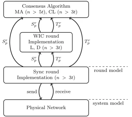
Figure 1 presents an overview of the consensus algo-rithms presented in the paper. The upper layer is the round-based Byzantine consensus algorithm (MA or CL) and is discussed in Sect. 3.1. Our consensus algorithms require eventually a phase where all rounds aresynchronous, and the first round isconsistent. Eventually synchronous rounds are provided by the implementation of the round model, which is discussed in Sect.4(third layer from top in Fig.1). En-suring eventually consistent rounds can be done in a leader-based (L) or decentralized (D) way, and is discussed in Sect. 3.2(second layer from top in Fig.1). By combining two consensus algorithms with two WIC round implementa-tions we get four algorithms that will be analyzed in Sect.5.
Fig. 1 Overview of the Byzantine consensus algorithms (the arrows
represent function calls;Sr
pandTprare the sending and transition func-tions introduced in Sect.2.2)
3.1 Consensus algorithms with WIC rounds
3.1.1 The MA algorithm
The MA algorithm [3,13] (Algorithm1) is inspired by the FaB Paxos algorithm proposed by Martin and Alvisi [12].3 A phaseφof Algorithm1 consists of two rounds: 2φ−1 and 2φ. Each process p has a state consisting of its cur-rent estimate xp, initially its initial value, and its decision decisionp, initially⊥. In round 2φ−1, processes first ex-change their estimate (line 6) and if they receive at least n−tmessages (line8), then they adopt the smallest most of-ten value received (line9). In round 2φ, processes exchange their new estimate (line12) and can decide if at leastn−t messages are the same (lines14–15). The algorithm is safe witht < n/5. For termination, there must be a phase, where both rounds are eventually synchronous and the first round is a WIC round.
Agreement follows from the fact that once a process de-cided, at least n−2t correct processes have the same es-timate x, and thus no other value will ever be adopted in line9. A similar argument is used for validity. Termination follows from the fact that in a round 2φ−1≥GSR with a consistent reception vectorμr all correct processes adopt the same value in line9, and thus decide on this value in round 2φ.
3FaB Paxos is expressed using “proposers”, “acceptors” and
Algorithm 1The MA algorithm withn >5t (code of pro-cessp) [3,13]
1: State:
2: xp∈V /*Vis the set of initial values */
3: decisionp∈V
4: Roundr=2φ−1: /* WIC round */
5: Spr:
6: sendxp to all processes
7: Tpr:
8: ifnumber of non-⊥elements inμrp≥n−tthen 9: xp←smallest most frequent non-⊥element inμrp
10: Roundr=2φ: 11: Sr
p:
12: sendxp to all processes
13: Tr p:
14: ifn−telements inμr
pare equal tov=⊥then
15: decisionp←v
3.1.2 The CL algorithm
The CL algorithm [3,13] (Algorithm2) is inspired by the PBFT algorithm proposed by Castro and Liskov [4], ex-pressed using rounds, including one WIC round.4
Algorithm 2consists of a sequence of phases φ, where each phase has three rounds: 3φ−2, 3φ−1, 3φ. Each pro-cessp has an estimatexp, a vote valuevotep (initially ?), a timestamp tsp attached to votep (initially 0), and a set pre-votepof valid pairsvote,ts (initially∅). Processes ex-change some of their state variables in every round. The structure of the algorithm is as follows:
– If a correct process p receives the same estimate v in round 3φ−2 fromn−t processes by line 14, then it acceptsvas a valid vote and putsv, φ inpre-votep set by line15. The prevote set is used later to detect an invalid vote (lines28–30).
– If a correct processp receives the same pre-votev, φ in round 3φ−1 fromn−t processes by line20, then it votesv (i.e.,votep←v) and updates its timestamp toφ (i.e.,tsp←φ) by line21.
– If a correct process preceives the same vote v with the same timestampφin round 3φfrom 2t+1 processes by line26, it decidesvin line27.
The algorithm guarantees that (i) two correct processes do not vote for different values in the same phaseφ; and (ii) oncet+1 correct processes have the same votev and the same timestampφ, no other value can be voted in the fol-lowing phases.
The algorithm is safe witht < n/3. For termination, the three rounds of a phase must eventually be synchronous and the first round must be a WIC round.5
4PBFT solves a sequence of consensus instances withweak validity,
while CL solves consensus withstrong validity.
5The proofs are given in [3].
Algorithm 2The CL algorithm withn >3t (code of pro-cessp) [3,13]
1: State:
2: xp∈V /*V is the set of initial values */
3: pre-votep← ∅
4: votep∈V∪ {?}, initially ?
5: tsp←0
6: decisionp∈V
7: Roundr=3φ−2: /* WIC round */
8: Spr:
9: sendxp,votep to all processes
10: Tpr:
11: ifat leastn−telements inμrpare equal to−,? then 12: xp←smallest most frequent elementx,− inμrp
13: pre-votep←pre-votep∪ {xp, φ }
14: ifat leastn−telements inμr
pare equal tov,− then
15: pre-votep←pre-votep∪ {v, φ }
16: Roundr=3φ−1: 17: Srp:
18: sendv| v, φ ∈pre-votep to all processes
19: Tpr:
20: ifat leastn−telements inμrpare equal tov then 21: votep←v;tsp←φ;xp←v
22: Roundr=3φ: 23: Sr
p:
24: sendvotep,tsp,pre-votep to all processes
25: Tr p:
26: ifat least 2t+1 elements inμr
pare equal tov=?, φ,− then
27: decisionp←v
28: ifexistsv=?, t s,− inμrps.t.votep=vandt s >tspthen
29: ifexistst+1 elements−,−,pre-vote inμr
ps.t.v,ts ∈
pre-voteandts≥tsthen 30: votep←?;tsp←0;xp←v
31: ifvotep=?thenxp←votep
3.2 Implementation of a WIC round
We consider two implementations for a WIC round: one leader-based and one decentralized. The implementations are also expressed using rounds. In order to distinguish them from the “normal” rounds, we useρto denote these rounds. The implementation has to be understood as follows. Letr be a WIC round, e.g., round r=2φ−1 of Algorithm 1. The messages sent in roundr=2φ−1 are used as the input variablempin the WIC implementation (see Algorithm3). The resulting vector provided by the WIC implementation, denoted byMp(Algorithm3) is then passed to the transition function of roundras the reception vectorμrp.
3.2.1 Leader-based implementation
Algorithm 3Leader-based implementation of a WIC round withn >3t (code of processp) [13]
1: Initialization:
2: ∀q∈Π: receivedp[q] ← ⊥
3: Roundρ=1: 4: Spρ:
5: sendmp to all processes
6: Tpρ:
7: receivedp←μρp
8: Roundρ=2: 9: Spρ:
10: sendreceivedp tocoordp 11: Tpρ:
12: ifp=coordpthen
13: for allq∈Πdo
14: if|{q∈Π:μρp[q][q] =receivedp[q]}|<2t+1then
15: receivedp[q] ← ⊥
16: Roundρ=3: 17: Spρ:
18: sendreceivedp to all processes
19: Tpρ:
20: for allq∈Πdo
21: if (μρp[coordp][q] = ⊥) ∧ |{i ∈ Π : μρp[i][q] =
μρp[coordp][q]}| ≥t+1then 22: Mp[q] ←μρp[coordp][q] 23: else
24: Mp[q] ← ⊥
ρ=3 is synchronous, all processes receive the same set of messages from this process in roundρ=3.
In round ρ=2, the coordinator compares the value re-ceived from some process p with the value indirectly re-ceived from other processes. If at least 2t+1 same values have been received, the coordinator keeps that value, other-wise it sets the value to⊥. This guarantees that if the co-ordinator keepsv, at leastt+1 correct processes have re-ceived v from p in round ρ=1. Finally, in round ρ=3 every process sends values received in roundρ=1 or⊥to all. Each process verifies whether at least t +1 processes validate the value that it has received from the coordinator in roundρ=3. Roundsρ=1 andρ=3 are used to verify that a faulty leader cannot forge the message from another process (integrity).
Since a WIC round can be ensured only with a correct coordinator, we need to ensure that the coordinator is even-tually correct. In Sect.4we do so by using arotating coordi-nator. A WIC round using this leader-based implementation needs three “normal” rounds.
3.2.2 Decentralized implementation
Algorithm4 is a decentralized (without leader) implemen-tation of a WIC round [3]. It implements a WIC round if eventually allt+1 rounds are synchronous. It is based on theExponential Information Gathering(EIG) algorithm for
Algorithm 4Decentralized implementation of a WIC round withn >3t(code of processp) [3]
1: Initialization:
2: Wp← {λ, mp }
3: Roundρ, 1≤ρ≤t+1: 4: Spρ:
5: send{α, v ∈Wp : |α| =ρ−1∧p /∈α∧v= ⊥}to all processes
6: Tpρ:
7: for all{q| α, v ∈Wp∧ |α| =ρ−1∧q∈Π∧q /∈α}do
8: ifβ, v is received from processqthen 9: Wp←Wp∪ {βq, v }
10: else
11: Wp←Wp∪ {βq,⊥ }
12: ifρ=t+1then
13: for allα, v ∈Wpfrom|α| =tto|α| =1do
14: Wp←Wp\ α, v
15: if∃vs.t.|αq, v ∈Wp| ≥n− |α| −tthen 16: Wp←Wp∪ α, v
17: else
18: Wp←Wp∪ α,⊥
19: for allq∈Πdo
20: Mp[q] ←vs.t.q, v ∈Wp
synchronous systems proposed by Pease, Shostak and Lam-port [14]. Initially, processphas its initial valuempgiven by the first round of the consensus algorithm (e.g., round 2φ−1 in Algorithm1). Throughout the execution, processes learn about the initial values of other processes. The infor-mation can be organized inside a tree. Each node of the tree constructed by processphas a label and a value (represented as a pairlable,value ). The root has an empty labelλand a valuemp. Process p maintains the tree using a setWp. Whenpreceives a messageβ, v fromq addsβq, v to Wp, otherwise it addsβq,⊥ . Aftert+1 rounds, badly-formatted messages inWpare dropped, and all correct pro-cesses have the same values inWp.
Similarly to the leader-based implementation, Algo-rithm 4requires n >3t. On the other hand, a WIC round using this decentralized implementation needst+1 “nor-mal” rounds.
3.3 The four combinations
Table 1 Performance of algorithms in terms of number of rounds
Best case Worst case
MA-D t+2 t+2
MA-L 4 4(t+1)
CL-D t+3 t+3
CL-L 5 5(t+1)
4 Round implementation
As already mentioned in Sect.2.1, we consider a partially synchronous system with an unknown boundδ on the end-to-end transmission delay between correct processes. The main technique to find the unknownδin the literature is us-ing an adaptive timeout, i.e., startus-ing the first phase of an algorithm with a small timeout Γ0 and increasing it from
time to time. The timeout required for an algorithm can be calculated based on the boundδand the number of rounds needed by one phase of the algorithm. The approach pro-posed in [7] is to increase the timeout linearly, while recent works, e.g., PBFT [4], increase the timeout exponentially.
The main question is when to increase the timeout. In-creasing the timeout in every phase provides a simple so-lution, in which all processes adopt the same timeout for a given phase. However, this is not an efficient solution, since processes might increase the timeout unnecessarily. An efficient solution is increasing the timeout when a correct process requires that. This occurs typically when a correct process is unable to terminate the algorithm (i.e., decide) with the current timeout. The problem with this solution is that different processes might increase the timeout at differ-ent points in time. Therefore, an additional synchronization mechanism is needed in this case.
For leader-based algorithms, a related question is the re-lationship between leader change and timeout change. Most of the existing protocols apply both timeout and leader mod-ifications at the same time [1, 4,6, 7, 9,12]. Our round implementation allows decoupling timeout modification and leader change. We show that such a strategy performs better than the traditional strategies in the worst case.
4.1 The algorithm
Algorithm5describes the round implementation. The main idea of the algorithm is to synchronize processes to the same round (round synchronization). The algorithm also re-quires view synchronization (eventually processes are in the same view) in addition to the round synchronization. This is because processes might increase the timeout at different rounds. The view number is thus used to synchronize the processes’ timeout.
Each process p keeps a round number rp and a view number vp, initially equal to 1. While the round number
Algorithm 5A round implementation for Byzantine faults withn >3t(code of processp)
1: rp←1;next_rp←1 /* round number */
2: Rcvp← ∅ /* set of received messages */
3: ∀i∈N: statep[i] ← ⊥ /* state of instancei*/
4: ∀i∈N: startp[i] ←0 /* starting round for instancei*/
5: vp←1;next_vp←1 /* view number */
6: whiletruedo
7: coordp←p(vp−1modn)+1 8:
input
&
send
I←input() 9: for alli, v ∈Ido 10: statep[i] ←init(v)
/* initialization of state with initial valuev*/
11: startp[i] ←rp
12: for alli: statep[i] = ⊥do
13: msgs[i] ←Sprp(statep[i],coordp)
14: for allq∈Πdo
15: Mq← {i,msgs[i][q] : statep[i] = ⊥ }
16: send(START, Mq, vp, rp, p)toq
17:
recei
v
e
timeoutp←current_time+Γ (vp)
18: whilenext_vp=vpandnext_rp=rpdo
19: ifcurrent_time≥timeoutpthen
20: send(INIT, vp, rp+1, p)to all
21: receive(M)
22: Rcvp←Rcvp∪M
23: if∃randt+1qs.t.INIT, vp, r+1, q ∈Rcvpthen
24: letr0be the largest suchr 25: ifr0≥rpthen
26: next_rp←r0
27: send(INIT, vp, r0+1, p)to all
28: if∃vandt+1qs.t.INIT, v+1,−, q ∈Rcvpthen
29: letv0be the largest suchv 30: ifv0≥vpthen
31: next_vp←v0
32: send(INIT, v0+1, rp, p)to all
33: if∃2t+1qs.t.INIT, vp, rp+1, q ∈Rcvpthen
34: next_rp←max{rp+1,next_rp}
35: if∃2t+1qs.t.INIT, vp+1,−, q ∈Rcvpthen
36: next_vp←max{vp+1,next_vp}
37:
comp.
&
output
O← ∅
38: for alli: statep[i] = ⊥do 39: for allr∈ [rp,next_rp−1]do
40: ∀q∈Π: Mr[q] ←m
if∃MSTART, M, vp, r, q ∈Rcvp∧ i, m ∈M elseMr[q] ← ⊥
41: statep[i] ←Tpr(Mr,statep[i],coordp)
42: if∃vs.t.decision(statep[i])=vthe first timethen 43: O←O∪ i, v /*vis the decision of instancei*/
44: output(O)
45: ifvp=next_vp ∧next_rpmodα=1then
46: if∃i:startp[i] ≤next_rp−α ∧ decision(statep[i])= ⊥ then
47: send(INIT, vp+1,next_rp, p)to all
48: rp←next_rp
49: vp←next_vp
based on the rotating leader paradigm (line 7). Note that the value ofcoordpis ignored in decentralized algorithms. The timeout does not necessarily change whenever the view changes. After line7, a process starts theinput&sendpart, in which it queries the input queue for new proposals (using a functioninput(), line8), initializes new slots on thestate vector for each new proposal (line10), calls the send func-tion of all active consensus instances (line13), and sends the resulting messages (line16). The process then sets a time-out for the current round using a deterministic functionΓ based on its view numbervp(line17), and starts thereceive part, where it collects messages (line22). Basically, this part uses an init/echo message scheme for round synchronization based on ideas that appear already in [7,8,16]. The receive part is described later. Next, in thecomp.&outputpart, the process calls the state transition function of each active in-stance (line 41), and outputs any new decisions (line 44) using the functionoutput(). Finally, a check is done at the end of each phase, i.e., only ifnext_rpmodα=1 (line45), whereα represents the number of rounds in a phase. The check may lead to request a view change, therefore, the check is skipped if vp =next_vp (the view changes any-way). The check is whether all instances, started at the be-ginning of the phase, have decided (lines45–46). If not, the process concludes that the current view was not successful (either the current timeout was small or the coordinator was faulty), and it expresses its intention to start the next view by sending an INITmessage for viewvp+1 (line47).
The function init(v) (line 10) gives the initial state for initial value v of the consensus algorithm; respectively, decision(state)(line42) gives the decision value of the cur-rent state of the consensus algorithm, or⊥if the process has not yet decided.
Receive part To prevent a Byzantine process from increas-ing the round number and view number unnecessarily, the algorithm uses two different type of messages, INIT
mes-sages and STARTmessages. Processpexpresses the inten-tion to enter a new roundr or new view v by sending an INIT message. For instance, when the timeout for the cur-rent round expires, the process—instead of starting immedi-ately the next round—sends an INIT message (line20) and waits that enough processes timeout. If processpin round rp and view vp receives at least 2t+1 INIT messages for round rp+1 (line33), resp. viewvp+1 (line 35), it ad-vances to roundrp+1, resp. to viewvp+1, and sends an STARTmessage with current round and view (line16). If the process receivest+1 INITmessages for roundr+1 with r≥rp, it enters immediately round r (line 23), and sends an INIT message for roundr+1. In a similar way, if the process receives t+1 INIT messages for viewv+1 with v≥vp, it enters immediately viewv(line28), and sends an INITmessage for viewv+1.
Properties of Algorithm5 The correctness proofs of Al-gorithm 5 are given in Sect. 4.4. Here, we give the main properties of the algorithm:
1. If one correct process starts roundr(resp. viewv), then there is at least one correct process that wants to start round r (resp. view v). This is because at most t pro-cesses are faulty (see Lemma1).
2. If all correct processes want to start round r+1 (resp. view v+1), then all correct processes eventually start roundr+1 (resp. viewv+1). This is becausen−t≥ 2t+1 and lines33–36(see Lemma2).
3. If one correct process starts round r (resp. view v), then all correct processes eventually start roundr(resp. view v). This is because a correct process starts round r (resp. viewv) if it receives 2t+1 INITmessages for round r (resp. view v). Any other correct process in roundr< r(resp. viewv< v) will receive at leastt+1 INITmessages for roundr(resp. viewv). By lines23to 26, these correct processes will start roundr−1 (resp. viewv−1) and will send an INITmessage for roundr (resp. viewv), see line27. From item2, all correct pro-cesses eventually start roundr (resp. viewv). The com-plete proof is given by Lemmas3–5.
4.2 Timing properties of Algorithm5
Algorithm5ensures the following timing properties: 1. If process pstarts round r (resp. viewv)at timeτ,all
correct processes will start roundr(resp. viewv)by time τ +2δ. This is becausephas received 2t+1 INIT mes-sages for round r (resp. view v), at time τ. All correct processes receive at least t+1 INIT messages by time τ +δ, start roundr−1 (resp. viewv−1) and send an INITmessage for roundr (resp. viewv). This message takes at most δ time to be received by all correct pro-cesses. Therefore, all correct processes receive at least 2t+1 INITmessages by timeτ +2δ, and start roundr (resp. viewv). The complete proof is given by Lemma5. 2. If a correct processpstarts roundr(viewv)at timeτ, it will start roundr+1the latest by timeτ+3δ+Γ (v). By item 1, all correct processes start round r, by time τ +2δ. Then they wait for the timeout of roundr, which is Γ (v). Therefore, by timeτ +2δ+Γ (v) all correct processes timeout for roundr, and send an INITmessage for round r+1, which takesδ time to be received by all correct processes. Finally, the latest by timeτ+3δ+ Γ (v), processpreceives 2t+1 INITmessages for round r+1 and starts roundr+1. The complete proof is given by Lemma6.
We can make the following additional observation:
Table 2 Summary of different strategies
Strategy A B C
Γ (v) vΓ0 2v−1Γ0 2
v−1
t+1Γ0
all roundr messages from all correct processes before the expiration of the timeout(at timeτ+3δ). By item1, all correct processes start roundr, by timeτ +2δ. The message of roundr takes an additionalδ time. There-fore, a timeout of at least 3δensures the stated property. The complete proof is given by Lemma7.
4.3 Parameterizations of Algorithm5
We now discuss different adaptive strategies for the time-out valueΓ (vp). First, we consider the approach of [7]: in-creasing the timeout linearly (whenever the view changes). We will refer to this parameterizations by A. Then we con-sider the approach used by PBFT [4]: increasing the timeout exponentially (whenever the view changes). We will refer to this parameterization by B. Finally, we propose another strategy, which consists of increasing the timeout exponen-tially every t+1 views. In the context of leader-based al-gorithms, this strategy ensures that, if the timeout is large enough to terminate the started consensus instances, then a Byzantine leader will not be able to force correct processes to increase the timeout. We will refer to this last parameter-izations by C. These three strategies are summarized in Ta-ble2, wherev represents the view number andΓ0denotes
the initial timeout.
4.4 Correctness proofs of Algorithm5
In the sequel, letτGdenote the first time that the actual end-to-end transmission delay δ is reached. All messages sent beforeτGare received the latest by timeτG+δ. Letv0
de-note the largest view number such that no correct process has sent a STARTmessage for viewv0by timeτG, but some correct process has sent a STARTmessage for viewv0−1.
Let r0 denote the largest round number such that no
cor-rect process has sent a STARTmessage for roundr0by time
τG, but some correct process has sent a STARTmessage for roundr0−1. We prove the results related to the view
num-ber, similar results hold for round numbers:
Lemma 1 Let p be a correct process that sends message
START,−, v,−, p at some timeτ0,then at least one cor-rect process q has sent message INIT, v,−, q at time τ ≤τ0.
Proof Assume by contradiction that no correct process q has sent messageINIT, v,−, q . This means that a correct
process can receive at mostt messages INIT, v,−,− in line28. Therefore, no correct process executes line32, and no correct process starts viewvbecause of line35, which is
a contradiction.
Lemma 2 Let all correct processes p send message
INIT, v,−, p at some time τ0, then all correct pro-cesses p will send message START,−, v,−, p by time max{τ0, τG} +δ.
Proof If all correct processespsend messageINIT, v,−, p at some timeτ0, then all correct processes are in viewv−1
at timeτ0by lines45–47. A correct processqin viewv−1,
receives at leastn−t≥2t+1 messagesINIT, v,−, p by timeτ0+δifτ0≥τG, or by timeτG+δifτ0< τG. From lines35and36,qstarts viewvby timemax{τ0, τG} +δ.
Lemma 3 Every correct processpsends messageSTART, −, v0−1,−, p by timeτG+2δ.
Proof We assume that there is a correct processpwithvp= v0−1 at timeτG. This means thatp has received at least 2t+1 messagesINIT, v0−1,−,− (line35). Or at leastt+
1 correct processes are in viewv0−2 and have sent a
mes-sageINIT, v0−1,−,− . These messages will be received
by all correct processes the latest by timeτG+δ. Therefore, all correct processes in view< v0−1 receive at leastt+1
messages INIT, v0−1,−,− by time τG+δ, start view v0−2 (line31) and send a message INIT, v0−1,−,−
(line 32). These messages are received by all correct pro-cesses by timeτG+2δ. Becausen−t >2t, all correct pro-cesses receive at least 2t+1 messagesINIT, v0−1,−,−
by timeτG+2δ (line 35), start viewv0−1 (line36), and
send a messageSTART,−, v0−1,−,− (line16).
Lemma 4 Letpbe the first(not necessarily unique)correct process that sends messageSTART,−, v, r, p withv≥v0 at some timeτ≥τG.Then no correct process sends message
START,−, v+1,−,− before timeτ +Γ (v).Moreover, no correct process sends messageINIT, v+2,−,− before timeτ +Γ (v).
Proof For the START message, assume by contradiction that process q is the first correct process that sends mes-sage START,−, v +1,1, q before time τ +Γ (v). Pro-cess q can send this message only if it receives 2t +1 messagesINIT, v+1,−,− (line35), This means that at least t +1 correct processes are in view v and have sent INIT, v+1,−,− . In order to send INIT, v+1,−,− , a correct process takes at leastΓ (v)time in viewv(line19). So messageSTART,−, v+1,−, q is sent by correct pro-cessqat the earliest by timeτ+Γ (v). A contradiction.
Lemma 5 Letpbe the first(not necessarily unique)correct process that sends messageSTART,−, v,−, p withv≥v0 at some time τ ≥τG.Then every correct process q sends messageSTART,−, v,−, q by timeτ+2δ.
Proof Note that by the assumption, all view v≥v0
mes-sages are sent at or afterτG, and thus they are received by all correct processesδtime later. By Lemma4, there is no mes-sageSTART,−, v,−,− withv> vin the system before τ +Γ (v). Processpsends messageSTART,−, v,−, p if it receives 2t+1 messagesINIT, v,−,− (line35). This means that at leastt+1 correct processes are in viewv−1 and have sent messageINIT, v,−,− , the latest by timeτ. All correct processes in view<vreceive at leastt+1 mes-sages INIT, v,−,− the latest by time τ +δ, start view v−1 (line31) and sendINIT, v,−,− (line32) which is re-ceived at mostδtime later. Becausen−t >2t, every correct processq receives at least 2t+1 messagesINIT, v,−,− by time τ +2δ (line 35), start view v (line 36), and send messageSTART,−, v,−, q (line16).
Following two lemmas hold for round numbers.
Lemma 6 If a correct process p sends message
START,−, v, r, p at time τ > τG, it will send message
START,−, v, r+1, p the latest by timeτ+3δ+Γ (v).
Proof From Lemma5(similar result for round number), all correct processes q send message START,−, v, r, q the latest by time τ +2δ. Then they wait for the timeout of roundrwhich isΓ (v)(lines17and19). Therefore, by time τ +2δ+Γ (v) all correct processes timeout for roundr, and sendINIT, v, r+1, q message to all (line20), which takes δ time to be received by all correct processes. Fi-nally, the latest by timeτ+3δ+Γ (v), processpreceives n−t≥2t+1 messagesINIT, v, r+1,− and starts round
r+1 (line36).
Lemma 7 A timeoutΓ (v)≥3δ for round r ensures that if a correct process p sends message START,−, v, r, p to all at time τ ≥τG, it will receive all round messages
START,−, v, r, q from all correct processesq,before the expiration of the timeout(at timeτ+3δ).
Proof From Lemma5(similar result for round number), all correct processesq send messageSTART,−, v, r, q to all the latest by timeτ +2δ. The message of roundrtakes an additionalδtime. Therefore a timeout of at least 3δensures
the stated property.
Therefore, we have the following theorem.
Theorem 1 Algorithm5withn >3t ensures the existence of roundr0such that∀r≥r0:Psync(r).
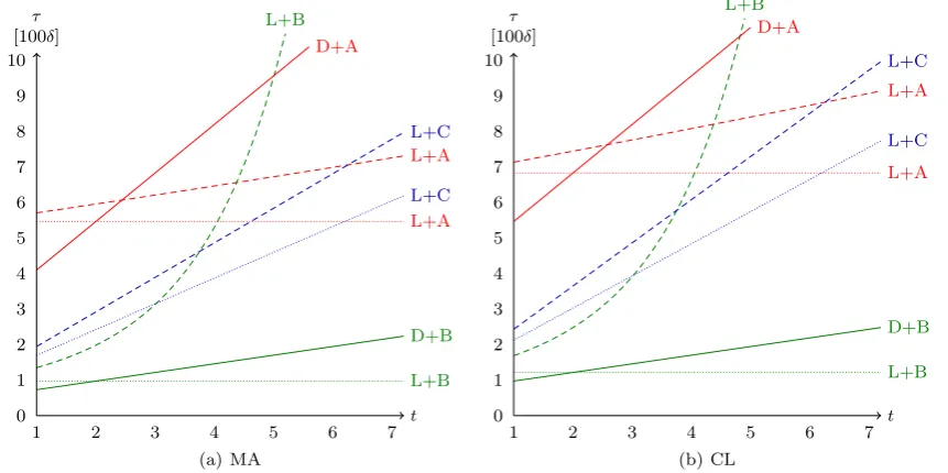
Table 3 Parameters for algorithms MA and CL
Fault-free case Worst case
α β α β
MA-D t+2 0 t+2 0
MA-L 4 0 4 t
CL-D t+3 0 t+3 0
CL-L 5 0 5 t
5 Timing analysis
In this section, we analyze the impact of the strategies A, B and C on our four consensus algorithms. We start with the analysis of the round implementation. Then we use these results to compute the execution time of k consecu-tive instances of consensus using the four algorithms MA-L, MA-D, CL-L, and CL-D.
First, for each strategy A, B, C, we compute the best case and worst-case execution time of k instances of repeated consensus, based on two parametersα andβ: The param-eterαis the one used in Algorithm 5. It denotes the num-ber of rounds per phase of an algorithm, i.e., the numnum-ber of rounds needed to decide in the best case. Thus,αgives also the length of a view in case a process does not decide. The parameterβ denotes the number of consecutive views in which a process might not decide although the timeout is already set to the correct value. This might happen when a faulty process is the leader. Table3shows the values forα andβ for our algorithms.
5.1 Best case analysis
In the best case we haveΓ0=δand there are no faults.
Pro-cesses start a round at the same time and a round takes 2δ (δ for the timeout and δ for the INIT messages), and pro-cesses decide at the end of each phase (=αrounds). There-fore, the decision for k consecutive instances of consen-sus occurs at time 2δαk. Obviously, the algorithm with the smallestα(that is, the leader-based or the decentralized with t≤2) performs in this case the best.
5.2 Worst case analysis
We compute now τX(k, α, β), the worst-case execution time until the kth decision when using the strategy X ∈ {A, B, C}. Based on item 3 in Sect. 4.2(and Lemma 7), the first decision does not occur until the round timeout is larger or equal to 3δ. We denote below withv0the view that
5.2.1 Strategy A
With strategy A, the timeout is increased in each new view byΓ0untilvΓ0≥3δ, i.e., untilv= 3δ/Γ0. Then the
time-out is increased for the next β views. Therefore, we have v0= 3δ/Γ0 +β. To compute the time until a decision,
ob-serve that a viewvlastsΓ (v)(timeout for viewv) plus the time until all INIT messages are received. It can be shown that the latter takes at most 3δ (see item 2 in Sect. 4.2). Therefore, we have for the worst case:
τA(1, α, β)= v0
v=1
αΓ (v)+3δ
=α v0
v=1
(vΓ0+3δ)=α
v0(v0+1)
2 Γ0+3δv0 =α Γ0 2
3δ/Γ0 +β
3δ/Γ0 +β+1
+3δ3δ/Γ0 +β
(1)
and fork >1,
τA(k, α, β)=τA(k−1, α, β)+α(v0Γ0+3δ)
=τA(k−1, α, β)
+α3δ/Γ0Γ0+βΓ0+3δ
. (2)
5.2.2 Strategy B
With strategy B, the timeout doubles in each new view un-til 2v−1Γ
0≥3δ. In other words, the timeout doubles until
reaching view v= log2Γ6δ0. Including β, we have v0= log2Γ6δ0 +β, and:
τB(1, α, β)= v0
v=1
αΓ (v)+3δ
=α v0
v=1
2v−1Γ0+3δ
=α2v0−1Γ
0+3δv0
=α2log2Γ6δ0+β−1Γ
0
+3δ log2
6δ Γ0 +β =α
2log2Γ3δ02β+1Γ
0−Γ0
+3δ log2
3δ Γ0
+3δ+3δβ
(3)
and fork >1,
τB(k, α, β)=τB(k−1, α, β)+α
2v0−1Γ0+3δ
=τB(k−1, α, β)+α
2log2Γ3δ02βΓ0+3δ.(4)
5.2.3 Strategy C
Finally, for strategy C, the timeout doubles in each new view until 2vt+1−1Γ0≥3δ. In other words, the timeout doubles until
reaching viewv=1+(t+1)log23Γδ
0; then it remains the same for the next β views. Therefore, we have and: v0=
(t+1)log2Γ3δ0 +β+1, and: 6
τC(1, α, β)
=α
(t+1)
v−1
t+1−1
l=0
2lΓ0+3δ
+(β+1)2vt+−11Γ0+3δ
=α(t+1)
2vt−+11Γ0−Γ0+3δv−1 t+1
+α(β+1)2vt+−11Γ0+3δ
=α(t+1)
2log2Γ3δ0Γ
0−Γ0+3δ log2
3δ Γ0
+α(β+1)2log2Γ3δ0Γ
0+3δ
(5) and fork >1,
τC(k, α, β)=τC(k−1, α, β)+α
2vt+−11Γ0+3δ(β+1) =τC(k−1, α, β)
+α2log2Γ30δΓ0+3δ(β+1). (6)
Note that strategy C makes sense only for leader-based al-gorithms.
5.2.4 Comparison
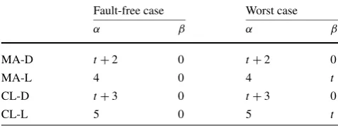
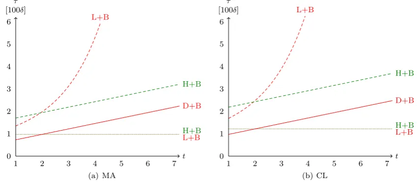
Table3givesαandβ for all algorithms we discussed. For the worst case analysis, we distinguish two cases: the worst fault-free case, which is the worst case in terms of the timing for a run without faulty process; and the generalworst-case that gives the values for a run in whichtprocesses are faulty. We compare our results graphically in Figs.2–4for algo-rithms MA and CL. The execution time for each algorithm and strategy is a function ofk,t, and the ratioδ/Γ0. In the
sequel, we fix two of these variables and vary the third. We first focus on the first instance of consensus, that is, we fix k = 1 and assume δ = 10Γ0 which gives
6Note that from v=1+(t+1)log
23Γδ0it follows that
v−1
t+1 is an
Fig. 2 Comparison fork=1.The dotted curverepresents the fault-free case andthe dashed curverepresents the worst case.The filled curve
represents both the fault-free case and the worst case
Fig. 3 Comparison fort=1.The dotted curverepresents the fault-free case andthe dashed curverepresents the worst case.The filled curve
represents both the fault-free case and the worst case
log2(3δ/Γ0) =5, i.e., the transmission delay is estimated
correctly after five times doubling the timeout. The result is depicted in Fig.2. We first observe, as expected, that the fault-free case and the worst-case are the same for the de-centralized versions (curves D+A and D+B). For the—in real systems relevant—cases t <3, for each strategy, the decentralized algorithm decides even faster in the worst-case than the leader-based version of the same algorithm in the fault-free case. For largert, the leader-based algorithms with strategy B, are faster in the fault-free case (L+B dotted curves), but less performant in the worst-case (L+B dashed curves). In the worst case, the execution time of leader-based algorithms with strategy B grows exponentially with
the number of faults. This shows the interest for strategy C (L+C dashed curves) in the worst case.
Fig. 4 Comparison of different strategies withk=1 andt=1.The dotted curverepresents the fault-free case andthe dashed curverepresents the worst case.The filled curverepresents both the fault-free case and the worst case
the most relevant caset=1. Again, we assumeδ=10Γ0.
Here, the decentralized algorithm is always superior to the leader-based variant using the same strategy, in the sense that even in the worst case it is faster than the correspond-ing algorithm in the fault-free case. In absolute terms, the decentralized algorithms with strategy B perform the best.
Finally, we analyze the impact of the choice ofΓ0on the
execution time (Fig. 4). This is relevant only for the first decision, i.e., k=1. We look at the case t =1 and vary log23Γδ0. Again, the decentralized version is superior for each strategy. However, it can be seen that strategy A is not a good choice, neither with a decentralized nor with a leader-based algorithm, if log23Γδ0 is too large. From this perspec-tive, strategy B is the best.
In all graphs, algorithm MA performs better than algo-rithm CL, since it requires less number of rounds, as shown in Table1. But both algorithms have similar behaviors.
6 Discussion
There are two important additional issues that we would like to emphasize before concluding the paper: the choice of the partial synchronous system model and the possibility to get a hybrid algorithm.
6.1 System model issue
The first issue is related to the round implementation. As we already mentioned, we consider a partially synchronous sys-tem where the end-to-end transmission delay is unknown. There are two variants in this model: (i) GST =0, or (ii) GST>0, where GST refers to the Global Stabiliza-tion Timeafter which the bounds on the message transmis-sion delay and process speed hold. In the first case, there
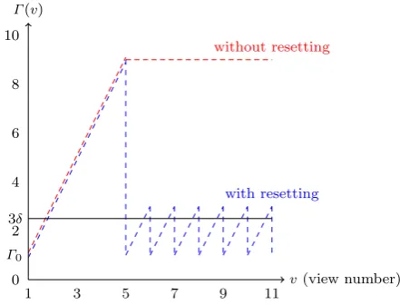
Fig. 5 Comparing different mechanisms for timeout
is no message loss, while in the second case there might be message loss beforeGST. Our round implementation (Algo-rithm5) is correct in both system models. However, it would not be efficient in the second model, since the timeout is in-creased beforeGST, and is never decreased. For the timing analysis in Sect.5 we have considered the first model. To obtain a more efficient round implementation in the second model, we suggest the following modifications:
1. Each correct process increases its timeout according to the timeout strategy until its first consensus decision. 2. Then the process asks to reset the timeout toΓ0by
send-ing aresetmessage.
3. If a correct process receives 2t+1resetmessages, it re-sets the timeout to the initial timeout, i.e.,Γ0.
4. If a correct process receivest+1resetmessages, it sends aresetmessage.
consen-Fig. 6 Comparison of hybrid algorithm fork=1 and strategy B.The dotted curverepresents the fault-free case andthe dashed curverepresents the worst case.The filled curverepresents both the fault-free case and the worst case
Table 4 Parameters for the hybrid algorithms
Fault-free case Worst case
α β α β
MA-H 4 0 t+6 0
CL-H 5 0 t+8 0
sus instance will require the same time as the first instance. In other words, we have the following formula for the worst-case execution time until thekth instance:
τX(k, α, β)=k·τX(1, α, β),
where τX(1, α, β) is given by the same formulas as in Sect.5.2.
Figure 5 compares the previous timeout mechanism (without resetting) with the mechanism presented in this section (with resetting). Assuming that GST holds at view number 5, the former keeps a larger timeout comparing to the latter.
6.2 Hybrid algorithm issue
The second issue is related to the leader-based versus de-centralized WIC round implementation. The leader-based version has better performance in the best case, while the decentralized version performs better in the worst case. By combining two approaches, we can obtain an algorithm that performs good in both cases. The idea is the following: in the first phase (or view) run the leader-based algorithm, i.e., MA-L or CL-L. If the first view is not successful, i.e., if there is a view change, then switch to the corresponding de-centralized algorithm, i.e., MA-D or CL-D.
Table4 shows the parameters for the hybrid algorithm (H refers to the hybrid algorithms).
Figure6 illustrates the results of the hybrid algorithms for strategy B, and compares them with the leader-based and decentralized algorithms. The hybrid algorithms are as good as the leader-based algorithms in the best case. In the worst case, the hybrid algorithms are much more efficient than the leader-based algorithm (fort ≥2), but not as good as the decentralized algorithms.
7 Conclusion
We compared the leader-based and the decentralized variant of two typical Byzantine consensus algorithms with strong validity in an analytical way using the same round imple-mentation.
Our analysis allows us to better understand the trade-off between the leader-based and the decentralized variants of an algorithm. The results show a surprisingly clear prefer-ence for the decentralized version. The decentralized vari-ant of algorithms has a better worst-case performance for the best strategy. Moreover, for the practically relevant cases t ≤2, the decentralized variant is at least as good as the fault-free case of the leader-based variant. Finally, in the best case, fort≤2, the decentralized variant is at least as good as the leader-based variant.
The results of our detailed timing analysis confirm the fact that the number of rounds is not necessarily a good es-timation of the performance of a consensus algorithm.
References
2. Ben-Or M (1983) Another advantage of free choice (ex-tended abstract): Completely asynchronous agreement proto-cols. In: PODC’83. ACM, New York, pp 27–30. doi:10.1145/ 800221.806707
3. Borran F, Schiper A (2010) A leader-free byzantine consensus al-gorithm. In: ICDCN. Lecture notes in computer science (LNCS). Springer, Berlin, pp 67–78
4. Castro M, Liskov B (2002) Practical Byzantine fault tolerance and proactive recovery. ACM Trans Comput Syst 20(4):398–461 5. Chandra TD, Toueg S (1996) Unreliable failure detectors for
reli-able distributed systems. J ACM 43(2):225–267
6. Clement A, Wong E, Alvisi L, Dahlin M, Marchetti M (2009) Making Byzantine fault tolerant systems tolerate Byzantine faults. In: NSDI’09. USENIX Association, Berkeley, pp 153–168 7. Dwork C, Lynch N, Stockmeyer L (1988) Consensus in the
pres-ence of partial synchrony. J ACM 35(2):288–323
8. Hutle M, Schiper A (2007) Communication predicates: a high-level abstraction for coping with transient and dynamic faults. In: Dependable systems and networks (DSN 2007). IEEE Press, New York, pp 92–100
9. Kotla R, Alvisi L, Dahlin M, Clement A, Wong E (2007) Zyzzyva: speculative byzantine fault tolerance. Oper Syst Rev 41(6):45–58. doi:10.1145/1323293.1294267
10. Lamport L (1998) The part-time parliament. ACMTCS 16(2):133–169
11. Lamport L, Shostak R, Pease M (1982) The byzantine gen-erals problem. ACM Trans Program Lang Syst 4(3):382–401. doi:10.1145/357172.357176
12. Martin JP, Alvisi L (2006) Fast Byzantine consensus. IEEE Trans Dependable Secure Comput 3(3):202–215. doi:10.1109/TDSC.2006.35
13. Milosevic Z, Hutle M, Schiper A (2009) Unifying byzantine con-sensus algorithms with weak interactive consistency. In: OPODIS, pp 300–314
14. Pease M, Shostak R, Lamport L (1980) Reaching agree-ment in the presence of faults. J ACM 27(2):228–234. doi:10.1145/322186.322188
15. Rabin M (1983) Randomized Byzantine generals. In: Proc sym-posium on foundations of computer science, pp 403–409 16. Srikanth TK, Toueg S (1987) Optimal clock synchronization.