O R I G I N A L A R T I C L E
Open Access
Initial impacts of the Ticket to Work program:
estimates based on exogenous variation in Ticket
mail months
David Stapleton
1, Arif Mamun
2*and Jeremy Page
3* Correspondence:
[email protected] 2Senior Research Economist and
Associate Director of Research, Mathematica Policy Research, 1100 First St NE, 12th Floor, Washington, DC 20002-4221, USA
Full list of author information is available at the end of the article
Abstract
This paper presents results from an impact analysis of the Ticket to Work (TTW) program, as implemented by the Social Security Administration (SSA) from 2002 through 2007. For new, young Social Security Disability beneficiaries, we use exogenous variation in the month of Ticket mailing to rigorously estimate impacts of TTW on beneficiary outcomes over a 48-month period following the start of Ticket mailings in the beneficiary’s state. We find substantial impacts on enrollment for employment services with TTW-qualified providers, but no consistent evidence of impacts on the number of months in which beneficiaries did not receive benefits because of work, or on other outcomes.
JEL classification:H55; I38
Keywords:Ticket to Work; Social Security disability benefits; Impact analysis; Voucher; Employment services
1. Introduction
The Old Age, Survivors and Disability Insurance system in the United States (OASDI, com-monly known as Social Security) offers disability insurance benefits to three groups of indi-viduals: workers who experience long-lasting medical impairments that prevent work at a substantial level (disabled workers), Disabled Adult Children (DAC) and Disabled Widow (er)s of other Social Security retired, deceased or disabled workers1. Collectively, these groups are called Social Security Disability (SSD) beneficiaries2. Many SSD beneficiaries with low SSD benefits also receive benefits from a separate welfare program, Supplemental Security Income (SSI), which is administered by the same agency, the Social Security Ad-ministration (SSA). In 2011, more than 9.8 million people received SSD benefits.
Many SSD beneficiaries are able and willing to work at some level; most of those who work earn too little to lose their benefits. Recognizing this, the Ticket to Work and Work Improvement Incentives Act of 1999 (Ticket Act) put into place a number of new policies and programs designed to encourage beneficiaries’return-to-work ef-forts. The leading initiative is the Ticket to Work (TTW) program. Initially, the Social Security Administration (SSA) mailed each eligible disability program beneficiary a “Ticket” that he or she could assign to either a state vocational rehabilitation agency (SVRA) or to a prequalified local rehabilitation service provider, called an employment network (EN), in exchange for employment placement, job training, and other
© Stapleton et al.; licensee Springer. This is an Open Access article distributed under the terms of the Creative Commons Attribution License (http://creativecommons.org/licenses/by/2.0), which permits unrestricted use, distribution, and reproduction in any medium, provided the original work is properly cited.
services3. SSA promised to pay the provider on the basis of earnings and benefit out-comes for the beneficiary. TTW was designed to expand the service options available to beneficiaries and create greater incentives for providers to help beneficiaries earn enough to forgo benefits.
TTW was rolled out in three phases. A first set of states completed the TTW rollout in 2002 (Phase 1), a second set in 2003 (Phase 2), and a final set in 2004 (Phase 3). In July 2008, SSA significantly changed the regulations governing TTW to attract more providers and reflect a more flexible return-to-work concept; hereafter, we call the pre-2008 program the“original”program.
Previous attempts to estimate impacts of TTW provide inconclusive evidence. The earlier analyses were, in essence, based on annual trends in differences for mean service enrollment, earnings and benefit outcomes across the three phases (Thornton et al. 2007; Stapleton et al. 2008). Results were inconclusive, because methodological issues made it impossible to discriminate between potentially very small, yet important im-pacts of TTW and pre-existing trends in the differences across phases for earnings and benefit outcomes. A number of alternative strategies were attempted in recent years to estimate Ticket impacts, but were also found to be inadequate4.
In this article, we present results from a rigorous new analysis of the impact of the introduction of the original TTW program, incorporating multiple innovations relative to earlier efforts. The analysis exploits a feature of the initial TTW rollout in each phase: just before the start of the rollout, SSA selected the month in which it intended to mail each eligible beneficiary’s Ticket in an essentially random fash-ion. We use variation in the intended mail month to rigorously estimate how the timing of Ticket mailing affects beneficiary outcomes over the following 48 months, then use the estimates to draw inferences about impacts of TTW (versus no TTW) over the same period. The new analysis also takes advantage of improve-ments in the measurement of work related outcomes from administrative data, namely a monthly indicator of benefit suspension or termination for work (STW) and a count of months in nonpayment status after STW (NSTW months) and be-fore returning to current-pay status, attainment of the full retirement age (FRA), or death (NSTW months)5. This article focuses on impacts for NSTW months as well as for two intermediate outcome variables: enrollment for employment ser-vices with an SVRA or EN, and an event that must precede STW: completion of the trial work period (TWP)6,7.
The findings reported here directly address the following primary research questions related to the three outcomes. Each question concerns the impact of duration from the month before the rollout start in the beneficiary’s state to the month in which SSA mailed a Ticket to the beneficiary (the beneficiary’s“mail month”) on outcomes over the 48 months after the rollout start.
Was enrollment for employment services and completion of TWP less likely to
occur as of 12, 24, 36, and 48 months after rollout start the longer the duration from rollout start to mail month?
Was the number of NSTW months as of 12, 24, 36, and 48 months after rollout
start smaller the longer the duration from rollout start to mail month?
We then use the findings to indirectly answer the question of most interest to policymakers:
What was the impact of mailing Tickets as of 48 months later versus not mailing
Tickets at all?
We also assess whether TTW was self-financing by 2007, before the new regulations took effect.
2. Data and methods 2.1. Ticket research file
We used data from the 2007 Ticket Research File (TRF07). The TRF is a set of analytic administrative data files constructed for the TTW evaluation. The TRF07 contains current and historical information on more than 22 million SSD beneficiaries or SSI recipients who received a benefit in at least one month from January 1996 through December 2007 (Hildebrand et al. 2009)8. For the purpose of this study, we constructed an analytic file for those awarded benefits from 1999 through 2003, based on the month that SSA first paid a benefit to the awardee9.
2.2. Analytic samples
2.2.1. Sample selection
The sample includes beneficiaries first awarded SSD benefits from July 1999 through October 2003. For the analysis, we followed each beneficiary for 48 months starting with the first month of the rollout in the beneficiary’s state. As the Phase 3 rollout started in November 2003, the last month in the sample is October 2007. We limit the analysis to this period because of factors external to the introduction of TTW. We started with July 1999 SSD awardees because this is the month in which the non-blind substantial gainful activity (SGA) level was increased from $500 to $700. We end the follow-up period in 2007 because of the severe recession that started in the last quarter of 2007 and because SSA made substantial changes to TTW regulations in 2008 that may have affected beneficiary outcomes in 2008 and later.
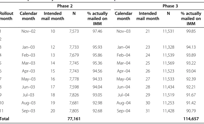
was SSA’s intent to mail Tickets to every beneficiary in these samples during a subse-quent rollout month (hereafter, the “intended mail month” [IMM]), to be determined by the terminal digit of the beneficiary’s SSN. Table 1 provides the sample sizes for each phase by IMM. Both phases follow identical 11-month schedules, except separated by 12 months, and mailings were uniformly distributed across 10 of the 11 rollout months, with the second month being the exception. As shown in Table 1, SSA mailed the vast majority of these Tickets on the IMM. Because the last four digits of SSNs are random conditional on age, the IMMs are essentially random. Thus, for each phase, we treat the samples defined by IMM (hereafter, the“IMM samples”) as randomly assigned sam-ples of those included on the phase’s selection date. This random assignment provided us with an exogenous source of variation—a variation over which the beneficiaries had no control—in the timing of Ticket mailing relative to program rollout start in each phase, which we use to identify the impacts of duration to Ticket mailing on benefi-ciary outcomes. As described later, the methodology also addresses the fact that some Tickets were not mailed on the IMM.
We also produced results for young, new SSD-only awardees selected for TTW rollout on January 12, 2002 (Phase 1), but two features of the Phase 1 rollout sub-stantially limit their value. The first such feature is that the Phase 1 sample had to be split into two relatively small samples because an operational issue led to differ-ent rollout schedules for New York (NY) and the rest of the Phase 1 states: the respective sample sizes in these two sample groups were 12,023 and 43,080, com-pared to 77,161 in Phase 2 and 114,657 in Phase 3. A second reason is that the rollout periods in Phases 2 and 3 (11 months in each) were substantially longer than in either part of Phase 1 (nine months in NY and five months in the rest of Phase 1). The larger samples and longer rollout periods in the later phases contrib-ute substantially to the ability of the methodology to detect small impacts. The Phase 1 findings do not contradict or illuminate the findings reported here, so have been omitted for brevity11.
Table 1 Sample sizes by intended mail months in phases 2 and 3
Phase 2 Phase 3
Rollout month
Calendar month
Intended mail month
N % actually mailed on
IMM
Calendar month
Intended mail month
N % actually mailed on
IMM
1 Nov–02 10 7,573 97.46 Nov–03 21 11,531 99.85
2
3 Jan–03 12 7,733 95.93 Jan–04 23 11,328 94.13
4 Feb–03 13 7,679 95.86 Feb–04 24 11,539 93.89
5 Mar–03 14 7,745 95.36 Mar–04 25 11,569 93.22
6 Apr–03 15 7,743 94.56 Apr–04 26 11,523 93.04
7 May–03 16 7,778 94.33 May–04 27 11,533 92.39
8 Jun–03 17 7,598 94.04 Jun–04 28 11,434 92.21
9 Jul–03 18 7,826 93.05 Jul–04 29 11,519 91.67
10 Aug–03 19 7,681 92.98 Aug–04 30 11,253 91.42
11 Sep–03 20 7,805 92.68 Sep–04 31 11,428 90.79
2.2.2. Intended and actual mail months
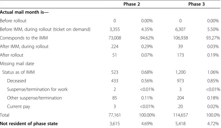
Although SSA actually mailed Tickets on the IMM for most beneficiaries, for a small fraction the actual mail month (MM) did not correspond to the IMM. The TRF records include the actual mail date, making it possible to determine the MM. Across the two phase-samples, in 93 to 95 percent of the cases the MM is the IMM. Although the frac-tion of Tickets mailed on the IMM was very high in each month of the rollout, it did decline in successive months. One reason for the decline is a provision of the regula-tions called“Ticket on demand”; beneficiaries in each phase could request a Ticket in advance of their mail date, and beneficiaries assigned to later IMM had more opportunity to make such requests a Ticket than those with early IMM. In addition, as the rollout progressed, SSA identified some beneficiaries who had died or were no longer in current-pay status, and consequently did not mail these bene-ficiaries their Tickets (see Table 2). Because mailing a Ticket on demand, mortality, and loss of current pay status for some other reason are likely predictive of the outcome variables, we made adjustments to the methodology to avoid confounding the correlation of these factors with the outcomes with the impacts of mailing the Ticket, as described in Section 2.3.
One other issue is that, in each phase, for a small share of beneficiaries (about 4.7 percent in each phase) the state of residence for the beneficiary obtained from the TRF was not among the states included in the phase’s rollout (Table 1). We do not know de-tailed reasons, but there are several possibilities: SSA included people in neighboring states that were served by a field office located in a state within the phase group; the state shown in the data reflects an address that is not the beneficiary’s own; or the beneficiary at some point moved to a non-phase state, but SSA did not know of this move on the selection date. Because we are aiming to retain as much of the original IMM sample as possible for the analysis, and because we found little variation in the percentage of the sample in each of these states across the mail months within phase, we did not exclude these cases12.
Table 2 Correspondence of actual mail months (MM) and intended mail months (IMM)
Phase 2 Phase 3
Actual mail month is—
Before rollout 0 0.00% 0 0.00%
Before IMM, during rollout (ticket on demand) 3,355 4.35% 6,307 5.50%
Corresponds to the IMM 73,008 94.62% 106,938 93.27%
After IMM, during rollout 224 0.29% 39 0.03%
After rollout 51 0.07% 173 0.19%
Missing mail date
Status as of IMM 523 0.68% 1,200 1.06%
Deceased 433 0.56% 973 0.85%
Suspense/termination for work 2 <0.01% 3 <0.01%
Other suspense/termination 85 0.11% 204 0.18%
Current pay 3 <0.01% 20 0.02%
Total 77,161 100.00% 114,657 100.0%
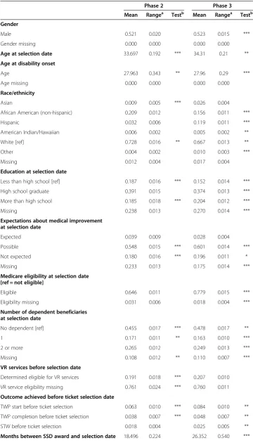
2.2.3. Beneficiary characteristics and tests of statistical equivalence
In Table 3, we present characteristics of the beneficiaries in the two phase samples. Al-most all of the characteristics are defined as of the beneficiary’s Ticket selection date. The exceptions are the primary disabling conditions, measured at SSD award date; the primary insurance amount, which is the earliest recorded value; and the indexed monthly earnings, also the earliest recorded value. The beneficiary populations vary somewhat across phases, as reflected in modest differences in means. Compared to the Phase 2 sample, the Phase 3 sample has relatively fewer African Americans (16 percent versus 21 percent), more Hispanics (12 percent versus3 percent), higher indexed monthly earnings ($1,125 versus $1,090) and Primary Insurance Amount (PIA)13($643 versus $632), and more beneficiaries with major affective disorders (18 percent versus 16 percent). Some of the differences reflect the fact that the Phase 3 rollout started 12 months after the Phase 2 rollout, so beneficiaries in Phase 3 had aged a year between the Phase 2 Ticket selection date and their own selection date, and more new awardees were added to the Phase 3 sample during the same period. For instance, compared to those in the Phase 2 sample, as of the selection date, they were older (mean of 34.3 ver-sus 33.7) and had been on the rolls longer (mean of 26 months verver-sus 18 months). In addition, those in the Phase 2 sample were more likely to have: previously enrolled for services, started the TWP, completed the TWP, experienced a month of suspension or termination for work, and become eligible for Medicare. In addition, some differences are expected between Phases 2 and 3 because of differences between the economic, policy and cultural environments for states in each phase.
Table 3 also presents tests of the statistical equivalence of the IMM samples within each phase. The statistical equivalence tests for each phase’s sample were conducted by running linear regressions of each characteristic on a set of IMM indicators for the months within that phase, without an intercept. For each regression, we conducted a joint test (an F-test) for the hypothesis that all of the population coefficients are equal. In conducting the test, we treated each state in the phase as a cluster and allowed for heteroscedasticity in the regression disturbance14. The F-tests show that we would re-ject the null hypothesis of“no difference”across IMM samples within phase for a large number of characteristics. Substantively, however, even when a baseline characteristic is found to be statistically different across IMM samples within a phase, variation in the means across the IMMs is not substantial, and does not appear to be correlated with the IMM. For example, in Phase 2, we found significant differences in mean beneficiary age at Ticket selection date across IMMs, but the difference between the maximum and minimum mean is 0.19 years around a mean for the phase of 33.70. There are also significant differences for some baseline values of the outcome variables. Most notably in Phase 2, 19.1 percent of beneficiaries had previously been found eligible for SVRA services, and the range of this percentage across the IMM was 1.8 percent. The distri-bution of the sample across states in each phase is not shown in Table 3 for brevity, but there were no statistically significant differences in state of residence by IMM for either phase15.
Table 3 Beneficiary characteristics: means by phase and intended mail months
Phase 2 Phase 3
Mean Rangea Testb Mean Rangea Testb
Gender
Male 0.521 0.020 0.523 0.015 ***
Gender missing 0.000 0.000 0.000 0.000
Age at selection date 33.697 0.192 *** 34.31 0.21 **
Age at disability onset
Age 27.963 0.343 ** 27.96 0.29 ***
Age missing 0.000 0.000 0.000 0.000
Race/ethnicity
Asian 0.009 0.005 *** 0.026 0.004
African American (non-hispanic) 0.209 0.012 0.156 0.011 ***
Hispanic 0.032 0.006 0.119 0.011 ***
American Indian/Hawaiian 0.006 0.002 0.005 0.002 **
White [ref] 0.728 0.016 ** 0.667 0.013 **
Other 0.004 0.002 0.010 0.003 ***
Missing 0.012 0.004 0.017 0.004
Education at selection date
Less than high school [ref] 0.187 0.016 *** 0.152 0.014 ***
High school graduate 0.391 0.015 0.374 0.013 ***
More than high school 0.185 0.018 *** 0.204 0.012 ***
Missing 0.238 0.013 0.270 0.014 ***
Expectations about medical improvement at selection date
Expected 0.039 0.009 0.028 0.004
Possible 0.548 0.015 *** 0.601 0.014 ***
Not expected 0.180 0.016 *** 0.196 0.011 *
Missing 0.233 0.013 0.175 0.014 ***
Medicare eligibility at selection date [ref = not eligible]
Eligible 0.646 0.011 0.779 0.015 ***
Eligibility missing 0.031 0.006 0.018 0.004 ***
Number of dependent beneficiaries at selection date
No dependent [ref] 0.455 0.017 *** 0.478 0.017 **
1 0.171 0.011 ** 0.163 0.010 ***
2 or more 0.265 0.012 0.249 0.013 ***
Missing 0.108 0.012 ** 0.110 0.007 ***
VR services before selection date
Determined eligible for VR services 0.191 0.018 *** 0.207 0.010
VR service eligibility missing 0.761 0.024 *** 0.760 0.011
Outcome achieved before ticket selection date
TWP start before ticket selection 0.063 0.010 *** 0.084 0.010 **
TWP completion before ticket selection 0.038 0.007 *** 0.048 0.007 **
STW before ticket selection 0.018 0.004 0.025 0.005 **
For this reason, it is important to control for these characteristics in the analysis—most critically, for the occurrence of the outcome events prior to Ticket selection date.
2.2.4. Outcome measures
The outcome measures are based on the 48 months starting with the first rollout month for the phase (month zero is the pre-rollout month). This period ends September 2006 for Phase 2, and September 2007 for Phase 3. For each individual in the sample we report re-sults for:
Two binary“event”variables. We determined when in the 48 months following
start of rollout each of the following events occurred, if at all: (1) enrolled for employment services (assigned their Ticket to an EN or were determined eligible for services by an SVRA); and (2) completed their last TWP month. In the analysis
Table 3 Beneficiary characteristics: means by phase and intended mail months
(Continued)
Primary Insurance Amount (PIA, $)
Mean PIA 626.9 18.8 * 643.3 12.3 ***
PIA missing 0.125 0.011 ** 0.123 0.009 ***
Indexed Monthly Earnings (IME, $)
Mean IME 1089.6 45.8 1124.9 28.4 ***
IME missing 0.192 0.009 0.185 0.008 **
Primary disabling conditions at SSD award
Major affective disorders [Ref] 0.155 0.018 *** 0.184 0.015
Other psychiatric disorders and mental retardation 0.241 0.019 ** 0.241 0.017 ***
Back disorders and musculoskeletal system 0.120 0.009 ** 0.111 0.011 ***
Other physical disabilities 0.482 0.027 *** 0.463 0.017 ***
Missing 0.001 0.001 0.001 0.001
SSD award year
1999 0.097 0.005 0.077 0.009 ***
2000 0.328 0.012 0.258 0.009
2001 0.300 0.012 * 0.293 0.014
2002 0.250 0.013 0.232 0.016 ***
2003 0.015 0.004 *** 0.128 0.015 ***
2004 0.009 0.003 * 0.012 0.003 ***
State unemployment rate
Mean in 6 months around IMM (percent) 5.710 0.385 *** 6.007 0.511 ***
Change in 6 months around IMM 0.079 0.843 *** −0.255 0.264 ***
Anomalous sequence of events
Ticket selection before SSD award 0.036 0.008 ** -
-TWP completion before start 0.000 0.001 0.000 0.000 ***
STW before TWP start 0.000 0.000 0.000 0.000 ***
STW before TWP completion 0.001 0.002 *** 0.001 0.001 ***
Source: Authors’calculations using data from Ticket Research File 2007.
Note:“Ref”indicates the reference category for the discrete variable in the multivariate regression models.
a“
Range”is the difference between the minimum and maximum mean across IMM in each sample.
b
of whether an event has occurred as of a specified rollout month (month 12, 24, 36, or 48), we define a binary variable for each event that is equal to one if the event occurred after the rollout start and before that month, and zero otherwise.
NSTW months, a count of the number of months in nonpayment status following
STW that occurred during the 48-month period. NSTW months include all months after benefits are suspended or terminated for work until the first of the following events occurs: (1) return to current-pay status, (2) suspension or termination for some other reason, or (3) the end of the 48-month period. Beneficiaries are not necessarily engaged in SGA during all NSTW months; we know only that they are not receiving benefits.
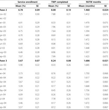
Means for the outcome variables in the IMM samples as of month 48 are presented in Table 4. The overall mean for Phase 2 is higher than Phase 3 for service enrollment, but the opposite is true for the other two outcomes. These differences reflect state dif-ferences in beneficiary characteristics, the labor market, and the support system, as well as the 12-month difference in time period.
Table 4 IMM sample percentages experiencing four events by end of month 48 after rollout start
Service enrollment TWP completed NSTW months
Mean (%) SE Mean (%) SE Mean (months) SE
Phase 2 6.78 0.09 8.08 0.10 1.460 0.024
Nov–02 7.25 0.30 7.88 0.31 1.412 0.074
Dec–02
Jan–03 6.91 0.29 8.33 0.31 1.470 0.075
Feb–03 6.72 0.29 7.96 0.31 1.597 0.079
Mar–03 6.75 0.29 7.64 0.30 1.394 0.072
Apr–03 6.70 0.28 8.69 0.32 1.483 0.075
May–03 6.78 0.28 8.15 0.31 1.472 0.074
Jun–03 6.69 0.29 8.08 0.31 1.542 0.079
Jul–03 6.45 0.28 8.01 0.31 1.448 0.074
Aug–03 6.46 0.28 8.06 0.31 1.357 0.072
Sep–03 7.07 0.29 7.99 0.31 1.423 0.075
Phase 3 5.67 0.07 8.24 0.08 1.686 0.021
Nov–03 5.90 0.22 8.33 0.26 1.645 0.065
Dec–03
Jan–04 5.73 0.22 8.76 0.27 1.750 0.068
Feb–04 5.84 0.22 8.22 0.26 1.617 0.064
Mar–04 5.67 0.22 8.17 0.25 1.641 0.065
Apr–04 5.39 0.21 8.17 0.26 1.668 0.066
May–04 5.54 0.21 8.45 0.26 1.756 0.067
Jun–04 6.09 0.22 8.26 0.26 1.733 0.068
Jul–04 5.55 0.21 7.78 0.25 1.675 0.067
Aug–04 5.46 0.21 8.17 0.26 1.672 0.066
Sep–04 5.57 0.21 8.12 0.26 1.703 0.067
The variation in service enrollment rates across IMM within each phase is consistent with a negative impact of duration to the mail month on enrollment as of month 48. For instance, for Phase 2, service enrollment declines from 7.25 percent for November 2002 to 7.07 percent for September 2003; the corresponding figures for Phase 3 are 5.90 and 5.57 percent. These differences are not statistically significant, however. The variation in means across IMM within each phase for other outcomes is not clearly consistent with negative impacts for those outcomes.
2.3. Estimation approach
2.3.1. Identification strategy
For each phase of the TTW rollout, SSA selected the IMM for all beneficiaries who were eligible on the phase’s Ticket selection date—approximately one month before rollout began. SSA used the terminal digit of the beneficiary’s SSN to determine the rollout month in which SSA would mail the beneficiary a Ticket. Because the last four digits (the serial numbers) of SSNs are considered to be random after conditioning on age16, this strategy essentially led to random assignment of the eligible beneficiaries to IMMs, after controlling for age. Consequently after controlling for age we assume that variation in the duration from the rollout start to the IMM is exogenous to each of the outcome variables (that is, independent of other unobserved factors that might affect outcomes). This provides the foundation for estimating the impacts of the duration from Ticket rollout start to the IMM on later beneficiary outcomes.
We used the exogenous assignment of IMMs to identify the impacts of delaying ac-tual Ticket mail month (MM) on beneficiary outcomes while accounting for a limited number of non-random deviations of the MM from the IMM. We hypothesize that the longer the duration from rollout start to the MM the lower the expected value for each outcome variable—enrollment in vocational services, completion of the TWP, and the number of NSTW months. The estimated impact of delaying the MM is expected to be different from the direct, intent-to-treat (ITT) impacts of delaying the IMM, and is likely to be of greater interest to policymakers17. The difference might be substantial because we are relying on random variation in duration from rollout start to the IMM to identify impacts, and the later a beneficiary’s IMM, the greater the likelihood of an adjustment to the actual MM. To produce these estimates, we use the IMM variables as instrumental variables (IV) for the MM variables18.
2.3.2. Instrumental variables estimation
To estimate the impact of actually mailing the Ticket on each outcome, we applied an IV approach to the following model:
MMi¼θIMMiþτXiþvi ð1Þ
Eit¼βt’MMiþyt’Xiþuit ð2Þ
24, 36, and 48 months following the rollout start. Because MMi is a vector, Equation (1) represents a set of equations, one for each mail month, andθ andτare both matri-ces. There is no intercept, becauseXicontains an exhaustive set of state indicators. For Equation (2), we restricted the coefficients of the exhaustive set of MM indicators to sum to zero in order to avoid exact collinearity. This normalization means that the co-efficient for each MM indicator is the predicted impact of Ticket mailing in that MM relative to mailing on the average MM during the rollout period (approximately 6.4 for both samples) (Suits1984). In other words, the normalization allows us to test the esti-mated impacts of mailing Ticket in each MM relative to the impact of mailing in the average MM.
Although we call MMithe actual mail month indicator vector, it does not indicate the actual mail month for every observation, because a small share of Tickets were never mailed, and an even smaller share were mailed shortly after the rollout window (that is, after the last month represented in MMi). In coding MMi, we had to choose one of the rollout period mail months for each of these observations in order to keep them in the sample. For each case, we chose a virtual month that is assumed to be con-sistent with the individual’s actual behavior. For the bulk of such cases—those never mailed a Ticket because of benefit termination prior to their IMM—we used the actual IMM on the assumption that had SSA proceeded to mail their Ticket on their IMMs, their behavior would have been the same as their actual behavior. That seems very likely, because they would have received their Ticket after they could no longer use them, and a large majority were deceased. For the very small share of cases in which the Ticket was mailed a few months after the rollout ended (0.07 percent for Phase 2 and 0.19 percent for Phase 3, as shown in Table 2), we chose the last rollout month; that is, we coded these late mailing cases as if their Tickets were mailed a few months earlier than they were actually mailed.
Two assumptions must be satisfied for IMMi to be a set of valid instruments. First, conditional on Xi, IMMi must be uncorrelated with the disturbance terms in Equations 1 and 2. Second, again conditional on Xi;IMMimust be correlated with the MMi. (Angrist et al. 1996). Both assumptions are satisfied in our case. The first as-sumption is plausible because SSA assigned IMM in a fashion that was exogenous with respect to the individual’s characteristics after conditioning on age; thus, by design, IMMiis independent of any unobserved individual characteristics. Further, the IMM se-lected could have no effect on the outcomes of interest except through its effect on the actual mailing of Tickets. The second assumption is satisfied because the vast majority of Tickets were mailed on the IMM (see Table 1). Hence, taken together, the IMMs constitute valid instruments for estimating the impact of the actual MM on beneficiary outcomes. Further, they are a very strong set of instruments, in that the correlation be-tween the IMM and MM variable for each mail month is quite high, reflecting the fact that the IMM and MM are identical in the vast majority of cases. This is also reflected in the very large F-statistic from the first stage of IV estimation for each endogenous MM, which ranged between 537 and 1,507 for Phase 2, and between 484 and 971 for Phase 3 for the MMs in each phase.
state level. These estimates also adjust for heteroskedasticity, which is expected because of the nature of the dependent variables. To test the null hypothesis that duration to MM has no impact on an outcome, we tested the hypothesis that all of the mail-month coefficients are zero. For each outcome, we also tested the hypothesis that the marginal impact of delaying the mailing of the Ticket an additional month was the same throughout the rollout period (that is, that there is a linear relationship between duration to mail month and the expected outcome). We used a chi-square test in each case.
3. Findings
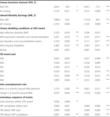
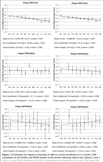
We present the IV estimates for the impacts of duration from rollout start to MM on service enrollment, TWP completion, and NSTW months graphically in Figure 1. Each panel in the figure shows the estimated impacts for each MM for the samples in Phase 2 (left panel) and Phase 3 (right panel). The mean value of the 10 point estimates in each phase is zero, by design; each point estimate measures the expected outcome for the sample mailed a Ticket in the corresponding month relative to the overall mean outcome for all those in the phase sample after accounting for pre-rollout characteris-tics and the fact that not all Tickets were mailed on schedule. In addition, we have plot-ted 95 percent confidence intervals around each point estimate (the short vertical line through each X) as well as the line obtained by constraining the IV estimates to fall on a straight line. The slope of the trend line indicates how much each one-month delay in mailing the Ticket affected the outcome. We also present two test statistics at the bottom of each panel: the first test statistic shows the result for the joint test of the null hypothesis that all the estimated IV coefficients are zero, and the second is for the lin-ear restrictions on the coefficients.
3.1. Clear evidence of impacts on service enrollment
As seen from the top panel of Figure 1, in both phases we found strong evidence of negative effects of duration to MM on service enrollment at 12 months following roll-out start in Phase 2 and Phase 3 (that is, the longer the duration, the lower the propor-tion enrolled). For both phases, the confidence intervals for the point estimates are narrow, the estimates steadily decline with duration, the data strongly reject the hy-pothesis that they are all zero, and fail to reject the hyhy-pothesis that the true values lie on a straight line. For Phase 2, the slope of the trend line is−0.084, indicating that each one-month delay in mailing the Ticket reduced the percentage enrolled in services as of month 12 by an estimated 0.084 percentage points, with a 95 percent confidence interval of ±0.033. Extrapolating to 12 months, the estimated impact on service enroll-ment at month 12 of mailing the ticket in month one versus not mailing it at all‒‒which is equivalent to the projected impact of a delay from month one to month 13‒‒is 1.0 percentage points (−0.084 × 12). The estimates suggest that the impact on ser-vice enrollment for Phase 3 was somewhat smaller than for Phase 2. The point estimate of the slope of the trend line is -0.066 (±0.025), and the projected impact on service enroll-ment at month 12 versus not mailing it at all is 0.8 percentage points. The difference be-tween the Phase 2 and Phase 3 slopes is not statistically significant, however.
-2.0 -1.5 -1.0 -0.5 0.0 0.5 1.0 1.5 2.0
Nov Dec Jan Feb Mar Apr May Jun Jul Aug Sep
) st ni o P e g at n e cr e P( M M f o ff e o C
Phase 2 SRV12 (IV)
-2.0 -1.5 -1.0 -0.5 0.0 0.5 1.0 1.5 2.0
Nov Dec Jan Feb Mar Apr May Jun Jul Aug Sep
Phase 3 SRV12 (IV)
Slope of Line =-0.084, SE =0.017, p-value < 0.001 Slope of Line = -0.066 SE = 0.013, p-value < 0.001
Zero Coefficients: Chi-sq(9) = 49.68, p-value < 0.001 Zero Coefficients: Chi-sq(9) = 51.2, p-value = 0.001
Linear Impacts: Chi-sq(7) = 6.50, p-value = 0.482 Linear Impacts: Chi-sq(7) = 6.02, p-value = 0.538
-2.0 -1.5 -1.0 -0.5 0.0 0.5 1.0 1.5 2.0
Nov Dec Jan Feb Mar Apr May Jun Jul Aug Sep Phase 2 TWPC48 (IV)
-2.0 -1.5 -1.0 -0.5 0.0 0.5 1.0 1.5 2.0
Nov Dec Jan Feb Mar Apr May Jun Jul Aug Sep Phase 3 TWPC48 (IV)
Slope of Line =-0.007, SE = 0.034, p-value = 0.842 Slope of Line =-0.041, SE = 0.019, p-value = 0.03
Zero Coefficients: Chi-square(9) = 21.11, p-value = 0.012 Zero Coefficients: Chi-square(9) = 23.02, p-value = 0.006
Linear Impacts: Chi-square(7) = 19.75, p-value = 0.006 Linear Impacts: Chi-square(7) = 12.95, p-value = 0.073
-0.20 -0.15 -0.10 -0.05 0.00 0.05 0.10 0.15 0.20
Nov Dec Jan Feb Mar Apr May Jun Jul Aug Sep
Co e ff o f M M ( M o n th s )
Phase 2 NSTW48 (IV)
-0.20 -0.15 -0.10 -0.05 0.00 0.05 0.10 0.15 0.20
Nov Dec Jan Feb Mar Apr May Jun Jul Aug Sep
C o e ff of M M (M ont h s )
Phase 3 NSTW48 (IV)
) st ni o P e g at n e cr e P( M M f o ff e o C ) st ni o P e g at n e cr e P( M M f o ff e o C ) st ni o P e g at n e cr e P( M M f o ff e o C
Slope of Line =-0.00595, SE = 0.00603, p-value = 0.324 Slope of Line = 0.00549, SE = 0.00541, p -value = 0.309
Zero Coefficients: Chi-square(9) = 17.85, p -value = 0.037 Zero Coefficients: Chi-square(9) = 22.88, p -value = 0.006
Linear Impacts: Chi-square(7) = 9.04, p -value = 0.250 Linear Impacts: Chi-square(7) = 14.43, p -value = 0.044
relationship between duration and service enrollment, but progressively weaker with the duration from rollout start to the observation month (see Stapleton et al. 2013 for details). This is consistent with expectations; as each month goes by, those mailed Tickets late in the rollout period have more time to catch up to those mailed Tickets earlier in terms of service enrollment. Thus, it appears that, on average, an early MM accelerated the beneficiary’s entry into service enrollment relative to a later MM, but service enrollment for those with later MM had, by the end of the observation period, largely caught up to enrollment for those with earlier MM.
3.2. Unclear evidence of impacts on TWP completion
The middle panel in Figure 1 plots the instrumental variable estimates for impacts on the likelihood of TWP completion at 48 months after the start of rollout, along with their 95 percent confidence intervals and estimated trend lines. Estimates for TWP completion at 12, 24 and 36 months appear in Stapleton et al. 2013 and are no stronger in terms of evi-dence of impacts than those at month 48. For both phases, the monthly estimates are jointly significant at the 5 percent level, but the patterns of monthly coefficients in each phase do not support the conclusion that their joint significance reflects an impact of dur-ation to MM on TWP completion. In each phase, the null hypothesis of zero coefficients is rejected primarily because estimates for two months have relatively large magnitudes (March and April for Phase 2 and January and July for Phase 3). For Phase 2 the pattern of the estimates is clearly inconsistent with a negative effect, and the slope of the trend line is very small and statistically insignificant. For Phase 3, the slope of the trend line is negative and significant at the 5 percent level, but the hypothesis that the impacts are lin-ear is rejected at the 10 percent level of significance. This leaves open the distinct possibil-ity that the estimates for Phase 3 are simply due to chance difference for the January and July samples rather than to a negative impact of duration to MM on TWP completion.
3.3. Unclear evidence of impacts on NSTW months
On the bottom panel in Figure 1, we plot the monthly IV estimates for impacts of duration to MM on the number of NSTW months completed as of 48 months after rollout start. The evi-dence from Phase 2 for NSTW months is marginally indicative of a substantive impact when viewed in isolation, but in the context of all of the findings—including lack of evidence for an impact in Phase 3—it seems equally plausible that the Phase 2 results simply reflect chance.
Interpretation of the Phase 2 results for NSTW months as indicative of impacts is also undermined by the evidence of impacts on TWP completion in the Phase 2 and 3 samples, described previously. We would not expect a negative impact on NSTW months unless there is a negative impact on TWP completion, as NSTW months can-not start until the TWP is completed. As described earlier, the evidence for an impact on TWP completion is very weak and, if anything, stronger for Phase 3 than for Phase 2. If we interpret the point estimates as impacts, we must conclude that an essentially zero impact on TWP completion for Phase 2 translated into a modest negative impact on NSTW months, while a modest negative impact on TWP months in Phase 3 trans-lated into a modest positive impact on NSTW months. An alternative explanation of these inconsistent results is that they are all due to chance. The analysis of total im-pacts, presented in the next section, reinforces the conclusion that the marginally sig-nificant impacts on NSTW months found for Phase 2 are simply the result of chance.
3.4. Projections of total impacts of TTW
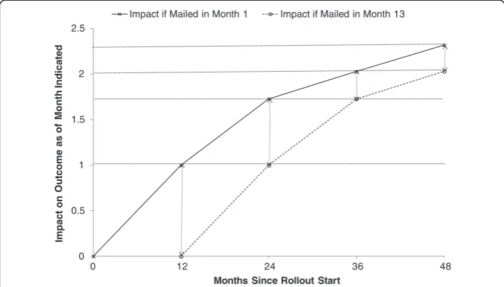
In this section we present projections of the impact of mailing Tickets in the first roll-out month versus never mailing them, as of 12, 24, 36 and 48 months later. These are derived from the estimates for the impacts of the duration to MM at 12, 24, 36 and 48 months under two important, but quite plausible and partially verifiable assumptions. We call these estimates projections because they rely on two maintained assumptions.
The first assumption is the“linearity”assumption: that the marginal impact of delay-ing the maildelay-ing of the Ticket on each outcome as of month 12, 24, 36, or 48 is linear through month 13 of the 48-month observation period for each sample. This assump-tion is clearly consistent with the acceptance of the linearity restricassump-tions for the service enrollment estimates as of month 12 (shown earlier) as well as analogous restrictions for months (24, 36 and 48—not shown). Linearity is sometimes rejected for TWP com-pletion and NSTW months, but in these cases it appears that rejection is due to one or two outlier estimates; the results for TWP completion at 48 months in Phase 2 and NSTW months in Phase 3 shown above are illustrative.
The second assumption is the “impact only delayed” assumption: that the impact of mailing the Ticket on each outcome for those mailed Tickets in month 13 is always exactly 12 months behind the impact on enrollment for those mailed Tickets in month one. For instance, the impact of mailing Tickets in month 13 as of month 24, 36, or 48 is exactly the same as the impact of mailing the Ticket in month one as of month 12, 24, or 36, respectively. This assumption is clearly consistent with the service enrollment point estimates for months 24, 36 and 48, which are progressively smaller than impacts at month 12, and which suggest that service enrollment for those mailed Tickets late in the rollout had essentially caught up to service enrollment for those mailed Tickets earlier (see Stapleton et al. 2013). This assumption is also not contradicted by the evidence for other outcomes, although for those outcomes there is not consistent evidence of impacts.
dashed line represents the total impact of mailing the Ticket in month 13 as of month 24, 36, and 48. The length of the vertical double arrow represents the impact of delay-ing the maildelay-ing from month 1 to month 13 at each observation point. The sum of the estimated impacts of mailing the Ticket at month 13 instead of month 1 as of months 12, 24, 36, and 48 (illustrated by the lengths of the four vertical arrows) is the total im-pact as of month 48 of mailing the Ticket in month 1 versus not mailing it at all.
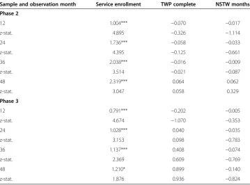
We applied this approach to all outcome variables in both phase samples. As illus-trated in Figure 2 and shown in Table 5, the projected impact on service enrollment at month 48 for Phase 2 is 2.3 percentage points and statistically significant. The corre-sponding projection for Phase 3 is a more modest 1.2 percentage points, but also sig-nificant. Another feature of the service enrollment projections is that the point estimates increase with the projection month in each phase—reflecting the maintained assumptions and the fact that the restricted IV estimates of all coefficients in the dur-ation to MM models are positive. Further, for Phases 2 and 3, the increment to the pro-jection diminishes with each 12-month period, as we would expect.
None of the projections for total impacts on other outcome variables are significant at even the 10 percent level as of any observation point. The NSTW-months estimates stand in stark contrast to those for service enrollment—the latter with uniformly positive point estimates and significant at the 0.10 level or better. These projections reinforce our earlier conclusion that there is no evidence of a substantial impact on any outcomes other than service enrollment.
3.5. Assessment of whether TTW was self-financing by 2007
The fact that we did not find statistically significant impacts on NSTW months does not by itself rule out the possibility that TTW under the initial regulations had impacts on these outcomes that were sufficiently large for the program to be “self-financing”— that is, for savings from a net reduction in benefits to be sufficient to pay for TTW pay-ments to providers and all administrative costs attributed to the program. Thornton (2012)
0 0.5 1 1.5 2 2.5
0 12 24 36 48
Indicated
Month
of
as
Outcome
on
Impact
Months Since Rollout Start
Impact if Mailed in Month 1 Impact if Mailed in Month 13
suggests that only a very small impact—an increase of 3,000 or so in the number of all beneficiaries experiencing suspension or termination for work (STW) for the first time in each year—might be sufficient for the program to be self-financing. Because this issue is critical to policymakers, in this section we assess in more detail whether the estimates are consistent with the self-financing hypothesis.
An impact of 3,000 is quite small relative to the number of first-time STW cases ac-tually observed in any recent year. Based on findings in Schimmel et al. (2013) and add-itional tabulations of their data, we estimate that an impact of 3,000 first STW cases is about five percent of the number of first STW cases in 2007 that would have occurred in the absence of TTW. An increase in STW of five percent would be sufficient for TTW to be self-financing only if NSTW increases by at least the same relative amount; if instead those who attain STW as the result of TTW return to the rolls quickly rather than accumulating NSTW months, reductions in benefits would be minimal.
Under certain strong assumptions, we could conclude that a TTW impact of five per-cent or greater on NSTW at 48 months for new, young SSD-only beneficiaries would be large enough to have made the program self-financing in 200719. The most problem-atic assumption is that 2007 can be interpreted as a steady state with respect to the number and characteristics of beneficiaries and their work activity. That assumption is required to interpret a cross-sectional impact of five percent in 2007 as the equivalent to a longitudinal impact of five percent for recent program entrants. In fact, 2007 was far from a steady state, primarily because the number of program entrants in the period leading up to 2007 was far larger than the number exiting the program. Because recent entrants are much more likely to enter STW and start to accumulate NSTW months
Table 5 Projected total impacts on service enrollment, TWP completion and NSTW months as of 12, 24, 36 and 48 months, by phase
Sample and observation month Service enrollment TWP complete NSTW months
Phase 2
12 1.004*** −0.070 −0.017
z-stat. 4.895 −0.326 −1.114
24 1.736*** −0.058 −0.033
z-stat. 4.395 −0.125 −0.661
36 2.038*** −0.016 −0.009
z-stat. 3.514 −0.021 −0.087
48 2.319*** 0.064 0.062
z-stat. 3.047 0.058 0.329
Phase 3
12 0.791*** −0.202 −0.005
z-stat. 4.674 −1.070 −0.353
24 1.028*** 0.040 −0.035
z-stat. 3.153 0.098 −0.783
36 1.137*** 0.408 −0.074
z-stat. 2.369 0.609 −0.769
48 1.210* 0.899 −0.140
z-stat. 1.876 0.936 −0.824
than those who have been on the rolls for many months (Liu and Stapleton 2011), we conclude that the longitudinal percentage impact on NSTW months for recent entrants would have to be substantially higher than five percent in order to achieve a cross-sectional impact of five percent in 2007.
For now, however, we treat the five percent figure as a lower bound and test the fol-lowing hypothesis: the mailing of Tickets to young, new SSD-only beneficiaries in-creased the number of NSTW months as of month 48 after the mailing by at least five percent versus the alternative hypothesis that the impact was less than five percent. We then consider how the results would change if the minimum percentage impact con-sistent with self-financing was larger than five percent, as it might well be.
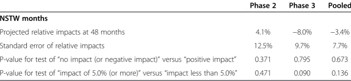
We use the projected total impacts in Phase 2 and 3 separately, and then, to increase power, we pool the results for the two phases on the assumption that the true relative impacts for the two phases are the same. The pooled projection is the minimum vari-ance projection under the assumption that percentage impacts were the same for Phases 2 and 320. Because of the inequalities in the null and alternative hypotheses, a one-tailed test is appropriate. Results appear in Table 6. We also show tests for the null hypothesis of“no impact”versus the one-tailed alternative of“positive impact”.
The statistical power of the projections for NSTW months is insufficient to rule out the possibility that TTW had impacts of at least five percent for Phases 2 and 3 pooled, but at the same time the evidence from these projections more consistent with zero or negative impacts than an impact of 5 percent or more. The percentage projections themselves are allsmallerthan 5 percent, and both the Phase 3 and pooled projections are negative (-8.0 percent and−3.4 percent, respectively). We cannot, however, reject the null hypothesis of a 5 percent impact based on the pooled sample (p-value of 0.14). Note, though, that the p-value for that test is much smaller than the p-value for the test of the null hypothesis that the true impact is zero or negative (0.67 percent). That is, the evidence is more consist-ent with the hypothesis of a zero or negative impact than with an impact of at least 5 percconsist-ent. As indicated above, the fact that 2007 followed a period of rapid program growth leads us to conclude that the smallest percentage impact for young SSD-only entrants that is consistent with self-financing is larger than five percent. If we had used a larger value in the tests above, the results would clearly be less favorable to the hypothesis of self-financing. For instance, a value of nine percent would lead to rejection of the hypothesis of financing at the five percent significance level using the pooled data. That is, if self-financing required at least a nine percent impact on NSTW months—a plausible value— we would have to reject the hypothesis that TTW was self-financing as of 2007.
Table 6 Projected relative impacts on NSTW months at 48 months after Ticket mailing
Phase 2 Phase 3 Pooled
NSTW months
Projected relative impacts at 48 months 4.1% −8.0% −3.4%
Standard error of relative impacts 12.5% 9.7% 7.7%
P-value for test of“no impact (or negative impact)”versus“positive impact” 0.371 0.795 0.673
P-value for test of“impact of 5.0% (or more)”versus“impact less than 5.0%” 0.471 0.090 0.136
4. Conclusion
We find clear evidence that the mailing of Tickets during the rollout period did in-crease service enrollment. The most important findings are captured in their implica-tions for the impact of Ticket mailing, versus no Ticket mailing, on service enrollment over the next 48 months. The Phase 2 and 3 findings are very significant and consistent with each other. The Phase 2 point estimates imply that the impact of mailing Tickets is 1.0 percentage points 12 months later, and 2.3 percentage points 48 months later. The corresponding estimates for Phase 3 are 0.8 and 1.2 percentage points. All of these estimates are very significant statistically. They are also large relative to what service enrollment would have been in the absence of ticket; the 48-month estimates imply relative impacts on the order of 50 percent and 25 percent for the two phases, respect-ively21. The point estimates are quite comparable to results from earlier impact analysis for SSD-only beneficiaries under age 40: a 0.6 percentage point increase in service en-rollment by the end of the rollout year and a 1.5 percentage point increase at the end of the following year (Thornton et al. 2007; Stapleton et al. 2008). Another feature of the findings is that, by month 48 after rollout start, service enrollment for those mailed Tickets late within each rollout period had essentially caught up with service enroll-ment for those who were mailed Tickets earlier in the rollout period.
The analysis provides no consistent evidence of impacts on other outcomes. Some es-timates for Phase 2 are suggestive of an impact, but it seems likely that they are due to chance. Specifically, marginally significant Phase 2 point estimates for NSTW months imply that a 12-month delay in mailing a Ticket decreases the number of NSTW months as of month 48 by an average of 0.07 months—approximately a five percent de-crease22. There are, however, substantial reasons to believe that these results are simply due to chance. The fundamental reason is the multiple comparisons problem; whenever an evaluation produces impacts for many outcomes, there are bound to be a few statis-tically significant findings by chance alone even if the intervention has absolutely no impacts. We have produced impact estimates for many different outcomes (not all in-dependent), so we would expect to find that some estimated impacts beyond those for service enrollment would be statistically significant even if there are no impacts on these outcomes. Hence, to assess whether the Phase 2 results for NSTW months reflect real impacts or simply chance, it is important to consider them in the context of all the estimates produced—are the latter consistent with real impacts for these outcomes in Phase 2?23In brief, the Phase 3 point estimate for the impact on NSTW months as of 48 months is positive, that is in the opposite direction found for Phase 2, and just as large. It is very hard to understand why comparable impacts on service enrollment in the two samples would translate into such different impacts for NSTW months. Fur-ther, the point estimates for the impact on TWP completion—a necessary precursor to accumulation of NSTW months—at 48 months is essentially zero for phase 2 and negative for Phase 3. Examination of the plots of coefficients for individual MM in Section 3 reveals that outlier estimates for early and late rollout months appear to ex-plain the estimated relationship between duration to MM and TWP completion for the two phase samples, rather than the impacts of Ticket mailing.
impacts on NSTW months that would be required for TTW to have been self-financing in 2007. Overall, however, the evidence is more consistent with no impact on NSTW months than with an impact large enough to make the program self-financing24.
The findings suggest that the early impacts of delaying Ticket mailing on service en-rollment did not translate into impacts on TWP completion and NSTW months. There are several possible explanations of this apparent disconnect. One is that TTW just in-creased observed service receipt without increasing actualservice receipt; because we only observe service enrollment with TTW-qualified providers (SVRA and EN), it might be that the expansion in providers resulted in an increase in receipt of services from TTW-qualified providers, but with no impact on total service receipt. Another possible explanation is that new services were provided to beneficiaries who were about to give up their benefits for work anyway. Findings from other research show that a large majority of beneficiaries forgo benefits for work without enrolling for services within SSA’s system (Schimmel et al. 2013). For such beneficiaries, the expansion of ser-vice availability under TTW represented an opportunity to obtain more serser-vices with-out changing their NSTW months. The nature of this opportunity is most apparent in the case of ENs offering “consumer-directed services”; these ENs pass through a large share of any payments received to the beneficiary. Services provided under TTW by other types of providers presumably also have substantial value to the beneficiary, even if they do not result in more NSTW months.
Our findings help explain the decline in the number of ENs accepting Ticket assign-ments from 2004 through 2007: they could not cover their costs from Ticket revenues alone. Because SSA payments to TTW providers are closely tied to the number of NSTW months its clients accumulate, a provider is unlikely to cover its cost unless it’s typical client accumulates many NSTW months, its costs are extremely low, or it has significant revenues from other sources. TTW providers during this period did receive some payments based on NSTW months, but our analysis suggests that this is primarily because they accepted Tickets from some clients that would have had NSTW months even in the absence of the TTW program; they were not able to increase the number of NSTW months of their clients. Thornton’s (2012) analysis of the economic viability of ENs confirms that, with the possible exception of consumer-directed ENs, providers were not able to cover their costs from ticket revenues alone during this period.
It is important to keep in mind that these estimates are for TTW under the original regulations. Reflecting concerns about the limited use of Tickets by beneficiaries and declining provider interest in Tickets, SSA attempted to rejuvenate the program by implementating significant regulatory changes in July 2008. The revisions: (1) increased the payments providers were eligible to receive from SSA if their clients achieved cer-tain earnings milestones without giving up their benefits; (2) increased the maximum amount that most providers are eligible to receive; (3) shortened the minimum period over which providers could receive the maximum amount from 60 months to 36 months; and (4) endorsed the use of the consumer-directed service model.
to SVRA—increased by 41 percent from 2007 to 2010 after increasing by just 8 percent from 2005 to 2007, and enrollments under the new payment systems alone increased by 377 percent.
In principle, the regulatory changes and consequent large growth in provider and beneficiary participation could have had a positive impact on NSTW months among all beneficiaries. However, it appears impossible to rigorously measure any such impact be-cause the new regulations were implemented nationwide in July 2008, just as the econ-omy was plunging into the deepest and longest recession since the 1956 inception of disability benefits under Social Security. Schimmel et al. (2013) found that the number of beneficiaries experiencing their first NSTW month fell from 74 thousand in 2007 to 53 thousand in 2009. It might be that the overall decline in beneficiaries experiencing a first NSTW month would have been worse in the absence of the regulatory changes, but we do not know. It might also be that the recession, rather than the regulations, ex-plains much of the increase in TTW participation; the recession no doubt made it more difficult to find jobs for many beneficiaries attempting to return to work, and some might well have sought assistance from a TTW provider as a result.
Our impact analysis for the pre-2008 period provides a lesson for SSA and other agencies when, in the future, they are asked to make a significant change to a large na-tional or state program—including significant future changes to TTW. Inasmuch as such a change often requires a lengthy rollout period, the agency should consider the knowledge that might be gained by implementing a rollout in which program partici-pants are randomly assigned an implementation month over a period of 12 months or so. This approach has its limits, however; it will not necessarily have sufficient power to identify substantively important impacts if such impacts are very small. Power can be increased if the program participants most likely to be affected by the change can be identified in advance, the rollout period can be lengthened, or a more extreme version of the change could be applied to randomly chosen participants. Such enhancements make this approach more like the approach that would be best from a purely methodo-logical perspective: a randomized control trial.
Endnotes 1
DAC receive benefits on the basis of a parent’s entitlement as a “primary benefi-ciary”—a parent who is a disabled worker, retirement beneficiary, or deceased worker. The DAC must be deemed unable to work as of the age of 22 under the same medical criteria applied to disabled workers, he or she is not entitled to benefits until the parent is entitled. Each disabled widow(er) beneficiary (DWB) receives benefits on the basis of the entitlement of a deceased spouse; the DWB must be at least 50 years old as well as meet the same medical criteria as disabled workers. DAC and DWB benefits are paid out of the Social Security Disability Insurance (SSDI) Trust Fund if the primary benefi-ciary is a disabled worker, or out of the Old Age and Survivors Insurance (OASI) Trust Fund if the primary beneficiary is a retiree or deceased. See SSA (2012) for further details.
2
3
SSA no longer mails tickets to beneficiaries. Instead, the beneficiary can approach a provider and the provider may contact SSA to verify eligibility.
4
A brief discussion of these alternative strategies is available in Stapleton et al. 2013. 5“
Current-pay”status means that the individual is eligible for a cash payment for the current month.
6
During the TWP, SSD beneficiaries are permitted to work and earn at any level with-out loss of benefits, provided that they continue to meet the medical eligibility require-ments. The TWP consists of 9 months, which need not be consecutive—any 9 months in a 60-month rolling window are counted. After completing the TWP, beneficiaries enter an extended period of eligibility (EPE). Except for a 3-month grace period, indi-viduals who engage in substantial gainful activity (SGA) in any of the next 36 months have their benefits suspended for that month. The beneficiary is entitled to full benefits during any month of this period when he or she is not engaged in SGA, provided that benefits have not been terminated for medical recovery or some other reason. After 36 months, SSD benefits are terminated in the first month of SGA after use of any remaining grace period months.
7
We also analyzed two other outcomes‒‒starting the TWP, and first month of benefit suspense or termination for work (STW)‒‒but their results are not essential to under-stand the key impacts of the TTW program. The results for these outcomes are avail-able in Stapleton et al. 2013.
8
Extracts from several Social Security administrative files were merged to create the TRF, including the Master Beneficiary Record, Supplemental Security Record, Numerical Identification System (Numident) file, the 831 and 832/33 Disability files, the Disability Control File, monthly snapshot files, and files from the payment history update system.
9
The first payment month (that is, the award month) is that in which the first pay-ment was actually made, which is usually after the first month for which the beneficiary is entitled to a benefit (that is, the entitlement month). The latter is often used in SSA’s statistics to classify beneficiaries by entry year (for example, SSA 2009). We use the award month instead because our focus is on the activities of beneficiaries once they become informed of their award and are entitled to use the DI work incentives.
10
SSA determined all beneficiaries who were eligible to receive a Ticket and who re-sided within the phase’s states as of the phase’s selection month. Almost all SSD benefi-ciaries and SSI recipients over age 18 were eligible; the main exceptions were (1) new beneficiaries with a status of medical improvement expected (MIE) who had not yet had their first medical continuing disability review (medical CDR) and (2) child SSI re-cipients who had reached age 18 and were waiting for redetermination as adults.
11
The Phase 1 findings are reported in Stapleton et al. (2013). 12
With a small number of cases in the “out-of-phase” states in each phase, the ran-dom variation at the state level may explain a substantial fraction of the variation in some characteristics across IMM samples. We address this issue in footnote 14 in the next section.
13
14
As noted earlier, because a small sample of beneficiaries are residents of “out-of-phase” states, each of which is treated as a cluster, it is conceivable that they might be substantially influencing the results of the joint tests of statistical equivalence. To ex-plore this, we conducted the joint tests without correcting for state-level clustering (but adjusting for heteroscedasticity) and found that we would reject the null hypoth-esis for far fewer characteristics. We suspect that with a small number of cases in the nontargeted states in each phase, the random variation in the cluster component of the model’s error term explains so much variation in some characteristics that tiny differ-ences across IMM groups are found to be significant. But this is just conjecture, and we are not aware of any technical problem with including a set of clusters with very small samples along with clusters that are much larger.
15
These statistics are available in Stapleton et al. (2013). 16
The serial numbers in SSNs are considered random only after conditioning on age because they are historically assigned in sequence (Barron and Bamberger 1982).
17
Estimates of direct impacts of delaying the IMM on beneficiary outcomes are avail-able in Stapleton et al. 2013.
18
As stated earlier, in order to address the fact that some Tickets were never mailed because benefits were suspended or terminated prior to the IMM, we coded the MM for those observations as if the Tickets were actually mailed on the IMM. We had pre-viously verified that, with almost no exceptions, termination or suspension of benefits had occurred for reasons other than work—most commonly mortality. Our reasoning for this modification is that mailing the Ticket to these beneficiaries during any month of the rollout would almost certainly have had no impact on their employment out-comes, in which case essentially all outcomes would have been the same as those ob-served had SSA mailed all of these Tickets in their IMM.
19
These assumptions are described and assessed in more detail in Stapleton et al. (2013, Appendix D).
20
The minimum variance estimate is a weighted mean of the estimates for the two phases where the weights have been chosen to minimize the variance of the estimate. More weight is given to the Phase 3 estimate for each impact because the Phase 3 esti-mate has lower variance than the Phase 2 estiesti-mate.
21
We used 4.5 percent as the counterfactual value for both phases, based on the fol-lowing calculations. The percentages enrolled at 48 months for the two phases are 6.8 and 5.7 percent. If we assume that as of month 48 the impacts for those mailed Tickets in later rollout months had caught up with impacts for those mailed Tickets in the first month, then these percentages would have both been 4.5 percent if the Ticket had never been mailed (6.8–2.3 and 5.7–1.2, respectively). The actual values are 51.1 and 26.7 percent larger than 4.5 percent, respectively.
22
The mean of NSTW months as of month 48 in Phase 2 is1.46 months. 23
There are formal ways to address the multiple comparison problem (see Schochet 2008, 2009). We have not conducted a more formal analysis because so few estimates other than those for service enrollment are even marginally significant.
24
months that beneficiaries had earnings above the TWP threshold, which is lower than the SGA amount ($640 in 2007 compared to $900 for SGA). This conclusion is rein-forced by a finding reported in Stapleton et al. (2013): that TTW had no significant im-pact on starting the TWP.
Competing interests
The IZA Journal of Labor Policy is committed to the IZA Guiding Principles of Research Integrity. The authors declare that they have observed these principles.
Acknowledgements
Research for this paper was carried out under the Ticket to Work Evaluation funded by SSA. We would like to thank: Paul O’Leary at SSA, for his guidance and forbearance as our project officer, and his reviews of earlier drafts; Jeff Smith, Hilary Hoynes, John Pepper, Peter Schochet, Jeff Hemmeter, Robert Weathers, Jim Sears, Elaine Gilby and Scott Muller for sound technical guidance; Dawn Phelps for her assistance in developing the data files; Maura Bardos for research assistance; and Craig Thornton, Yonatan Ben-Shalom, Gina Livermore, David Neumark and an anonymous referee for reviewing earlier drafts. The findings and conclusions presented in this article are those of the authors and do not necessarily represent the views of SSA or Mathematica Policy Research.
This paper was submitted to the IZA Journal of Labor Policy's call for papers on "Social Security Disability Benefits: Finding Alternatives to Benefit Receipt." Two special editors, David Wittenburg and Gina Livermore, were sponsored by the University of New Hampshire’s Rehabilitation, Research, and Training Center on Employment Policy and
Measurement, funded by the U.S. Department of Education (ED), National Institute on Disability and Rehabilitation Research (cooperative agreement no. H133B100030). Their comments do not necessarily represent the policies of ED or any other federal agency (Edgar, 75.620 (b)). The authors are solely responsible for all views expressed.
Responsible editor: David Neumark
Author details
1Senior Fellow and Director, Center for Studying Disability Policy, Mathematica Policy Research, 1100 First St NE, 12th
Floor, Washington, DC 20002-4221, USA.2Senior Research Economist and Associate Director of Research, Mathematica Policy Research, 1100 First St NE, 12th Floor, Washington, DC 20002-4221, USA.3Senior Programmer Analyst, Mathematica Policy Research, 1100 First St NE, 12th Floor, Washington, DC 20002-4221, USA.
Received: 6 October 2013 Accepted: 25 January 2014 Published:
References
Angrist J, Imbens G, Rubin D (1996) Identification of causal effects using instrumental variables. J Am Stat Assoc 91(434):444–455 Barron E, Bamberger F (1982) Meaning of the social security number. Soc Sec Bullet 45(11):29–30
Hildebrand L, Kosar L, Page J, Smither C, Loewenberg M, Phelps D, Justh N (2009) User’s guide for the Ticket research file TRF07: data from January 1994 to December 2007. Mathematica Policy Research, Washington, DC
Liu S, Stapleton D (2011) Longitudinal statistics on work activity and use of employment supports for new social security disability insurance beneficiaries. Soc Sec Bulletin 71(3):11–75
Mamun A, O’Leary P, Wittenburg D, Gregory J (2011) Employment among social security disability program beneficiaries: 1996-2007. Soc Sec Bulletin 71(3):11–34
Social Security Administration (2012) Annual statistical report on the Social Security Disability Insurance program, 2011. Social Security Administration, Washington, DC
Schimmel J, Stapleton D, Mann D, Prenovitz S, Phelps D (2013) Participant and provider outcomes since the inception of Ticket to Work and an assessment of the effect of the changes to the regulations in 2008: report submitted to the Social Security Administration. Mathematica Policy Research, Washington, DC
Schochet P (2008) Guidelines for multiple testing in impact evaluations of educational interventions: final report submitted to the U.S. Dep of Ed, Institute of Ed Sc. Mathematica Policy Research, Princeton, NJ
Schochet P (2009) An approach for addressing the multiple testing problem in social policy impact evaluations. Eval Rev 33(6):539–567
Stapleton D, Mamun A, Page J (2013) Initial impacts of the Ticket to Work program for young new Social Security disability awardees: estimates based on randomly assigned mail months. Mathematica Policy Research, Washington, DC
Stapleton D, Livermore G, O’Day B, Thornton C, Weathers R, Harrison K, O’Neil S, Sama Martin E, Wittenburg D, Wright D (2008) Ticket to Work at the crossroads: a solid foundation with an uncertain future: report submitted to the Social Security Administration. Mathematica Policy Research, Washington, DC
Suits D (1984) Dummy variables: mechanics v. interpretation. Rev of Econ Stat 66(1):177–180
Thornton C, Weathers R, Wittenburg D, Fraker T, Stapleton D, Gregory J, Mamun A (2007) Initial impacts of the Ticket to Work program on Social Security disability beneficiary service enrollment, earnings and benefits. J of Voc Rehab 27(2):129–140
Thornton C (2012) Can the Ticket to Work program be self-financing? Mathematica Policy Research, Washington, DC
Cite this article as:Stapletonet al.:Initial impacts of the Ticket to Work program: estimates based on exogenous variation in Ticket mail months.IZA Journal of Labor Policy
17 Mar 2014
10.1186/2193-9004-3-6