DOI 10.1007/s12651-013-0135-0 A RT I C L E
Estimation of standard errors and treatment effects in empirical
economics—methods and applications
Olaf Hübler
Published online: 10 July 2013
© Institut für Arbeitsmarkt- und Berufsforschung 2013
Abstract This paper discusses methodological problems of standard errors and treatment effects. First, heteroskedasti-city- and cluster-robust estimates are considered as well as problems with Bernoulli distributed regressors, outliers and partially identified parameters. Second, procedures to de-termine treatment effects are analyzed. Four principles are in the focus: difference-in-differences estimators, matching procedures, treatment effects in quantile regression analysis and regression discontinuity approaches. These methods are applied to Cobb-Douglas functions using IAB establishment panel data.
Different heteroskedasticity-consistent procedures lead to similar results of standard errors. Cluster-robust estimates show evident deviates. Dummies with a mean near 0.5 have a smaller variance of the coefficient estimates than others. Not all outliers have a strong influence on significance. New methods to handle the problem of partially identified param-eters lead to more efficient estimates.
The four discussed treatment procedures are applied to the question whether company-level pacts affect the output. In contrast to unconditional difference-in-differences and to estimates without matching the company-level effect is posi-tive but insignificant if conditional difference-in-differences, nearest-neighbor or Mahalanobis metric matching is ap-plied. The latter result has to be specified under quantile treatment effects analysis. The higher the quantile the higher is the positive company-level pact effect and there is a ten-dency from insignificant to significant effects. A sharp re-gression discontinuity analysis shows a structural break at a
O. Hübler (
)Institut für Empirische Wirtschaftsforschung, Leibniz Universität Hannover, Königsworther Platz 1, 30167 Hannover, Germany e-mail:huebler@ewifo.uni-hannover.de
probability of 0.5 that a company-level pact exists. No spe-cific effect of the Great Recession can be detected. Fuzzy regression discontinuity estimates reveal that the company-level pact effect is significantly lower in East than in West Germany.
Keywords Standard errors·Outliers·Partially identified parameters·DiD estimators·Matching·Quantile regressions·Regression discontinuity
JEL Classification C21·C26·D22·J53
Schätzung von Standardfehlern und Kausaleffekten in der empirischen Wirtschaftsforschung – Methoden und Anwendungen
Zusammenfassung Dieser Beitrag diskutiert Möglichkei-ten zur Schätzung von Standardfehlern und Kausaleffek-ten. Zunächst werden heteroskedastie- und gruppenrobus-te Schätzungen für Standardfehler betrachgruppenrobus-tet sowie Auffäl-ligkeitenund Probleme bei Dummy-Variablen als Regres-soren, Ausreißern und nur partiell identifizierten Parame-tern erörtert. Danach geht es um Verfahren zur Bestimmung von Treatmenteffekten. Vier Prinzipien werden hierzuvor-gestellt: Differenz-von-Differenzen-Schätzer, Matchingver-fahren, Kausaleffekte in der Quantilsregressionsanalyse und Ansätze zur Bestimmung von Diskontinuitäten bei Regres-sionsschätzungen. Anwendungen erfolgen im zweiten Teil der Arbeit auf Cobb-Douglas-Produktionsfunktionen unter Verwendung von IAB-Betriebspaneldaten.
Koeffizienterschätzer auf als andere. Nicht alle Ausreißer haben einen nennenswerten Einfluss auf die Signifikanz. Neuere Methoden zur Behandlung des Problems von nur partiell identifizierten Parametern führen zu effizienteren Schätzungen.
Die vier diskutierten Verfahren zur Bestimmung der Wir-kungen von Maßnahmen werden auf das Problem, ob be-triebliche Bündnisse einen signifikanten Einfluss auf den Produktionsoutput haben, angewandt. Im Gegensatz zu nicht konditionalen Differenz-von-Differenzen-Schätzern und Schätzern ohne Matching sind die Effekte betriebli-cher Bündnisse bei bedingten Differenz-von-Differenzen-Schätzern und Matching-Verfahren zwar positiv, aber in-signifikant. Diese Aussage ist auf Basis der Treatment-Quantilsanalysezu präzisieren. Je höher die Quantile sind, umso größer ist die Wirkung betrieblicher Bündnisse mit ei-ner Tendenz von insignifikanten zu signifikanten Effekten. Die deterministische Regressionsanalyse mit Diskontinui-täten zeigt einen Strukturbruch bei Wahrscheinlichkeit 0.5, dass ein betriebliches Bündnis existiert. Es lassen sich kei-ne spezifischen Effekte während der Rezession 2009 aus-machen. Schätzungen im Rahmen stochastischer Diskonti-nuitätsansätze offenbaren, dass die Wirkungen betrieblicher Bündnisse in Ostdeutschland signifikant niedriger ausfallen als in Westdeutschland.
1 Introduction
Contents, questions and methods have changed in empirical economics in the last 20 years. Many methods were devel-oped in the past but the application in empirical economics follows with a lag. Some methods are well-known but have experienced only little attention. New approaches focus on characteristics of the data, on modified estimators, on cor-rect specifications, on unobserved heterogeneity, on endo-geneity and on causal effects. Real data sets are not com-patible with the assumptions of classical models. Therefore, modified methods were suggested for the estimation and in-ference.
The road map of the following considerations are four hypotheses where the first two and the second two belong together:
(1) Significance is an important indicator in empirical eco-nomics but the results are sometimes misleading. (2) Assumptions’ violation, clustering of the data, outliers
and only partially identified parameters are often the reason of wrong standard errors using classical meth-ods.
(3) The estimation of average effects is useful but subgroup analysis and quantile regressions are important supple-ments.
(4) Causal effects are of great interest but the determination is based on disparate approaches with varying results.
In the following some econometric methods are developed, presented and applied to Cobb-Douglas production func-tions.
2 Econometric methods
2.1 Significance and standard errors in regression models
The working horse in empirical economics is the classical linear model
yi=xiβ+ui, i=1, . . . , n.
The coefficient vector β is estimated by ordinary least squares (OLS)
ˆ
β=XX−1Xy
and the covariance matrix by ˆ
V (β)ˆ = ˆσ2XX−1,
whereXis the design matrix andσˆ2the estimated variance of the disturbances. The influence of a regressor, e.g. xk, on the regressandy is called significant at a 5 percent level if |t| = | ˆβk/
ˆ
V (βˆk)|> t0.975. In empirical papers this re-sult is often documented by an asterisk and implicitly inter-preted as a good one, while insignificance is a negative sig-nal. Ziliak and McCloskey (2008) and Krämer (2011) have criticized this procedure although the analysis is extended by robustness tests in many investigations. Three types of mistakes can lead to a misleading interpretation:
(1) There does not exist any effect but due to technical in-efficiencies a significant effect is reported.
(2) The effect is small but due to the precision of the esti-mates a significant effect is determined.
(3) There exists a strong effect but due to the variability of the estimates the statistical effect cannot be detected. The consequence cannot be to neglect the instrument of sig-nificance. But what can we do? The following proposals may help to clarify why some standard errors are high and others low, why some influences are significant and others not, whether alternative procedures can reduce the danger of one of the three mistakes:
• Compute robust standard errors.
• Analyze whether variation within clusters is only small in comparison with variation between the clusters.
• Check whether dummies as regressors with high or low probability are responsible for insignificance.
• Detect whether collinearity is effective. • Investigate alternative specifications. • Use sub-samples and compare the results. • Execute sensitivity analyses (Leamer1985).
• Employ the sniff test (Hamermesh2000) in order to detect whether econometric results are in accord with economic plausibility.
2.1.1 Heteroskedasticity-robust standard errors
OLS estimates are inefficient or biased and inconsistent if assumptions of the classical linear model are violated. We need alternatives which are robust to the violation of specific assumptions. In empirical papers we find often the hint that robust standard errors are displayed. This is imprecise. In most cases this means only heteroskedasticity-robust. This should be mentioned and also that the estimation is based on White’s approach. If we know the type of heteroskedas-ticity, a transformation of the regression model should be preferred, namely
yi σi =
β0 σi +
β1 x1i
σi + · · · + βK
xKi σi +
ui σi ,
wherei=1, . . . , n. Typically, the individual variances of the error term are unknown. In the case of unknown and unspe-cific heteroscedasticity White (1980) recommends the fol-lowing estimation of the covariance matrix
ˆ
Vwhit e(β)ˆ =
XX−1uˆ2ixixi
XX−1.
Such estimates are asymptotically heteroscedasticity-robust. In many empirical investigations this robust estimator is rou-tinely applied without testing whether heteroskedasticity ex-ists. We should stress that those estimated standard errors are more biased than conventional estimators if residuals are ho-moskedastic. As long as there is not too much heteroskedas-ticity, robust standard errors are also biased downward. In the literature we find some suggestions to modify this esti-mator, namely to weight the squared residualsuˆ2i:
hc1= n n−Kuˆ
2
i
hcj= 1 (1−cii)δj
ˆ u2i,
where j = 2,3,4, cii is the main diagonal element of X(XX)−1X and δj =1;2;min[γ1, (ncii)/K] +min[γ2, (ncii)/K],γ1andγ2are real positive constants.
The intention is to obtain more efficient estimates. It can be shown forhc2that under homoskedasticity the mean of
ˆ
u2i is the same asσ2(1−cii). Therefore, we should expect that thehc2 option leads under homoskedasticity to better
estimates in small samples than the simplehc1option. Then E(uˆ2i/(1−cii)) isσ2. The second correction is presented by MacKinnon and White (1985). This is an approximation of a more complicated estimator which is based on a jack-knife estimator—see Sect.2.1.2. Applications demonstrate that the standard error increases started with OLS viahc1, hc2 to thehc3 option. Simulations, however, do not show a clear preference. As one cannot be sure which case is the correct one, a conservative choice is preferable (Angrist and Pischke2009, p. 302). The estimator should be chosen that has the largest standard error. This means the null hypoth-esis (H0: no influence on the regressand) keeps up longer than with other options.
Cribari-Neto and da Silva (2011) suggest γ1 =1 and γ2=1.5 in hc4. The intention is to weaken the effect of influential observations compared with hc2 and hc3 or in other words to enlarge the standard errors. In an earlier ver-sion (Cribari-Neto et al.2007) a slight modification is pre-sented:hc4∗=1/(1−cii)δ4∗, whereδ4∗=min(4, ncii/K). It is argued that the presence of high leverage observations is more decisive for the finite-sample behavior of the consis-tent estimators ofV (β)ˆ than the intensity of heteroskedas-ticity,hc4andhc4∗aim at discounting for leverage points— see Sect.2.1.5—more heavily thanhc2andhc3. The same authors formulate a further estimator
hc5= 1 (1−cii)δ5ˆ
u2i,
where δ5=min(ncKii,max(4,nkcKii,max)), k is a predefined constant, wherek=0.7 is suggested. In this case squared residuals are affected by the maximal leverage.
2.1.2 Re-sampling procedures
Other possibilities to determine the standard error are the jackknife and the bootstrap estimator. These are re-sampling procedures, which construct sub-samples withn−1 obser-vations in the jackknife case. Sequentially, one observation is eliminated. The former methods compare the estimated coefficients of the total sample sizeβˆwith those after elim-inating one observationβˆ−i. The jackknife estimator of the covariance matrix is
ˆ Vjack=
n−K n
n
i=1
(βˆ−i− ˆβ)(βˆ−i− ˆβ).
of the coefficients the asymptotic covariance matrix is
ˆ Vboot=
1 B
B
b=1 ˆ
β(b)m− ˆβ
ˆ
β(b)m− ˆβ
,
where βˆ is the estimator with the original sample size n. Alternatively, βˆ can be substituted byβ¯=1/Bβ(b)ˆ m. Bootstrap estimates of the standard error are especially help-ful when it is difficult to compute standard errors by conven-tional methods, e.g. 2SLS estimators under heteroskedastic-ity or cluster-robust standard errors when many small clus-ters or only short panels exist. The jackknife can be viewed as a linear approximation of the bootstrap estimator. A fur-ther popular way to estimate the standard errors is the delta
method. This approach is especially used for nonlinear
func-tions of parameter estimatesγˆ =g(β). An asymptotic ap-ˆ proximation of the covariance matrix of a vector of such functions is determined. It can be shown that
n1/2(γˆ−γ0)∼N
0, G0V∞(β)Gˆ 0
,
whereγ0is the vector of the true values ofγ,G0is anl× Kmatrix with typical element∂gi(β)/∂βj, evaluated atβ0, and V∞ is the asymptotic covariance matrix ofn1/2(βˆ− β0).
2.1.3 The Moulton problem
The variance of a regressor is low if this variable strongly varies between groups but only little within groups (Moul-ton1986,1987,1990). This is especially the case if indus-try, regional and macroeconomic variables are introduced in a microeconomic model or panel data are considered. In a more general context this is called the problem of clus-ter sampling. Individuals or establishments are sampled in groups or clusters. Consequence may be a weighted esti-mation that adjust for differences in sampling rates. How-ever, weighting is not always necessary and estimates may understate the true standard errors. Some empirical investi-gations note that cluster-robust standard errors are displayed but do not mention the cluster variable. If panel data are used then this is usually the identification variable of the individ-uals or firms. In many specifications more than one cluster variable, e.g. a regional and an industry variable, is incor-porated. Then it is misleading if the cluster variable is not mentioned. Furthermore, then a sequential determination of a cluster-robust correction is not qualified if there is a de-pendency between the cluster variables. If we can assume that there is a hierarchy of the cluster variables then a multi-level approach can be applied (Raudenbush and Bryk2002; Goldstein2003). Cameron and Miller (2010) suggest a two-way clustering procedure. The covariance matrix can be de-termined by
ˆ
Vtwo-way(β)ˆ = ˆV1(β)ˆ + ˆV1(β)ˆ − ˆV1∩2(β)ˆ
when the three components are computed by ˆ
V (β)ˆ =XX−1BˆXX−1 ˆ
B= G
g=1
XguˆguˆgXg
.
Different ways of clustering can be used. Cluster-robust in-ference asymptotics are based onG→ ∞. In many applica-tions there are only a few clusters. In this caseuˆghas to be modified. One way is the following transformation
˜ ug=
G G−1uˆg.
Further methods and suggestions in the literature are pre-sented by Cameron and Miller (2010) and Wooldridge (2003).
A simple and extreme example shall demonstrate the cluster problem.
Example Assume a data set with 5 observations (n=5) and 4 variables (V1–V4).
i V1 V2 V3 V4
1 24 123 −234 −8
2 875 87 54 3
3 −12 1234 −876 345
4 231 −87 −65 9808
5 43 34 9 −765
The linear model
V1=β1+β2V2+β3V3+β4V4+u
is estimated by OLS using the original data set (1M). Then the data set is doubled (2M), quadrupled (4M) and octupli-cated (8M). The following OLS estimates result.
ˆ β
1M 2M 4M 8M
ˆ
σβˆ σˆβˆ σˆβˆ σˆβˆ
V2 1.7239 1.7532 0.7158 0.4383 0.2922
V3 2.7941 2.3874 0.9747 0.5969 0.3979
V4 0.0270 0.0618 0.0252 0.0154 0.0103
const 323.2734 270.5781 110.463 67.64452 45.0963 The coefficients of 1M to 8M are the same, however, the standard errors decrease if the same data set is multiplied. Namely, the variance is only 1/6, 1/16 and 1/36 of the orig-inal variance. The general relationship can be shown as fol-lows. For the original data set (X1) the covariance matrix is
ˆ
V1(β)ˆ = ˆσ12
X1X1 −1
UsingX1= · · · =XF theF times enlarged data set with the design matrixX=:(X1· · ·XF)leads to
ˆ
σF2= 1 F ·n−K
F·n
i=1 ˆ
u2i =F (n−K) F ·n−Kσˆ
2 1
and ˆ
VF(β)ˆ = ˆσF2
XX−1= ˆσF2 1 F ·
X1X1
−1
= n−K
F ·n−KVˆ1(β).ˆ
Kis the number of regressors including the constant term,n is the number of observations in the original data set (num-ber of clusters),F is the number of observations within a cluster. In the numerical example withF =8,K=4,n=5 the Moulton factorMF that indicates the deflation factor of the variance is
MF = n−K
F ·n−K = 1 36.
This is exactly the same as it was demonstrated in the nu-merical example. Analogously the estimated values 1/6 and 1/16 can be determined. As the multiplying of the data set does not add any further information to the simple original data set not only the coefficients but also the standard er-rors should be the same. Therefore, it is necessary to correct the covariance matrix. Statistical packages, e.g. Stata, sup-ply cluster-robust estimates
ˆ V (β)ˆ C=
C
c=1 XcXc
−1C
c=1
XcuˆcuˆcXc C
c=1 XcXc
−1 ,
whereC is the number of clusters. In our specific case this is the number of observationsn. This approach implicitly assumes thatF is small andn→ ∞. If this assumption does not hold a degrees-of-freedom correction
dfC= F·n−1
F·n−K · n n−1
is helpful. dfC· ˆV (β)ˆ Cis the default option in Stata and cor-rects for the number of clusters in practice being finite. Nev-ertheless, this correction eliminates only partially the under-estimated standard errors. In other words, the corrected t-statistic of the regressorxkis larger than that ofβˆk/
ˆ V1k.
2.1.4 Large standard errors of dichotomous regressors with small or large mean
Another problem with estimated standard errors can be in-duced by Bernoulli distributed regressors. Assume a simple two-variable classical regression model
y=a+b·D+u.
Dis a dummy variable and the variance ofbˆis
V (b)ˆ =σ 2
n · 1 sD2,
where
sD2 = ˆP (D=1)· ˆP (D=0)=: ˆp(1− ˆp) = (n|D=1)
n ·
1−(n|D=1) n
.
IfsD2 is determined by D¯ =(n|D=1)/n we find that ¯
Dis at most 0.5.V (b)ˆ is minimal at givennandσ2 when the sample variance ofDreaches the maximum, ifD¯ =0.5. This result holds only for inhomogeneous models.
Example An income variable (Y=Y0/107) with 53,664 ob-servations is regressed on a Bernoulli distributed random variable RV. The coefficient β1 of the linear model Y = β0+β1RV+uis estimated by OLS, where alternative val-ues of the mean ofRV (RV) are assumed (0.1,0.2, . . . ,0.9)
Y βˆ1 std.err.
RV =0.1 −0.3727 0.6819
RV =0.2 −0.5970 0.5100
RV =0.3 −0.4768 0.4455
RV =0.4 0.3068 0.4170
RV =0.5 0.1338 0.4094
RV =0.6 0.0947 0.4187
RV =0.7 −0.0581 0.4479
RV =0.8 −0.1860 0.5140
RV =0.9 −0.1010 0.6827
This example confirms the theoretical result. The standard error is smallest ifRV =0.5 and increases systematically if the mean of RV decreases or increases. An extension to multiple regression models seems possible—see applica-tions in theAppendix, Tables11,12,13,14. The moreD¯ deviates from 0.5, the larger or smaller is the mean of D, the higher is the tendency to insignificant effects. A caveat is necessary. The conclusion that thet-value of a dichoto-mous regressorD1is always smaller than that ofD2, when V (D1) > V (D2), is not unavoidable. The basic effect ofD1 onymay be larger than that ofD2ony. The theoretical re-sult aims on specific variables and not on the comparison be-tween regressors. In practice, significance is determined by t= ˆb/
ˆ
than that of a company-level pact (CLP). The coefficients of the former regressor are larger and the standard errors are lower than that of the latter regressor so that thet-values are larger. In both cases the standard errors increase if the mean of the regressor is reduced. The comparison of line 1 in Ta-ble13with line 9 in Table14, where the mean of CLP and WOCO is nearly the same, makes clear that the stronger ba-sic effect of WOCO on lnY dominates the mean reduction effect of WOCO. Thet-value in line 9 of Table14is smaller than that in line 1 of Table14but still larger than that in line 1 of Table13. Not all deviations of the mean of a dummy Das regressor from 0.5 induce the described standard error effects. A random variation ofD¯ is necessary. An example, where this is not the case, is matching—see Sect. 2.2and the application in Sect. 3. D¯ increases due to the system-atic elimination of those observations with D=0 that are dissimilar to those ofD=1 in other characteristics.
2.1.5 Outliers and influential observations
Outliers may have strong effects on the estimates of the co-efficients, of the dependent variable and on standard errors and therefore on significance. In the literature we find some suggestions to measure outliers that are due to large or small values of the dependent variable or on the independent vari-ables. Belsley et al. (1980) use the main diagonal elements ciiof the hat matrixC=X(XX)−1Xto determine the ef-fects of a single observation on the coefficient estimatorβˆ, on the estimated endogenous variableyˆiand on the variance
ˆ
V (y). The higherˆ cii, the higher is the difference between the estimated dependent variable with and without the ith observation. A rule of thumb orients on the relation
cii> 2K
n .
An observationiis called an influential observation with a strong leverage if this inequality is fulfilled. The effects of theith observation onβˆ,yˆandV (ˆ β)ˆ and the rules of thumb can be expressed by
βˆk− ˆβk(i)> 2 √ n
yˆi− ˆyi(i) s(i)√cii >2
K
n
det(s2(i)(X(i)X(i))−1 det(s2(XX)−1)
>3K
n .
If the inequalities are fulfilled, this indicates a strong influ-ence of observation i where(i) means that observation i
is not considered in the estimates. The determination of an outlier is based on externally studentized residuals
ˆ
u∗i = uˆi s(i)√1−cii
∼tn−K−1.
Observations which fulfill the inequality| ˆu∗i|> t1−α/2;n−K−1 are called outliers. Alternatively, a mean shift outlier model can be formulated
y=Xβ+Ajδ+, where
Aj=
1 ifi=j 0 otherwise.
Observationjhas a statistical effect onyifδis significantly different from zero. The estimatedt-value is the same asuˆ∗j. This procedure does not separate whether the outlierjis due to unusualy- or unusualx-values.
Hadi (1992) proposes an outlier detection with respect to all regressors. The decision whether the design matrixX contains outliers is based on an elliptical distance
di(c, W )=
(xi−c)W (xi−c),
where intuitively the classical choices ofc andW are the arithmetic mean (x) and the inverse of the sample covariance¯ matrix (S−1) of the estimation function ofβ, respectively, so that the Mahalanobis distance follows. If
di
¯
x, S−12> χK2,
observation i is identified as an outlier. As x¯ andS react sensitive to outliers it is necessary to estimate an outlier-free mean and sample covariance matrix. For this purpose, only outlier-free observations are considered to determine
¯
2.1.6 Partially identified parameters
Assume that some observations are unknown or not exactly measured. Consequence is that a parameter cannot exactly be determined but only within a range. The outlier situation leads to such a partial identification problem. There exist many other similar constellations.
Example The share of unemployed persons is 8 % but 5 %
have not answered to the question of the employment status. Therefore, the unemployment rate can only be calculated within certain limits, namely between the two extremes: • all persons who have not answered are employed • all persons who have not answered are unemployed. In the first case the unemployment rate is 7.6 % and in the second case 12.6 %.
The main methodological focus of partially identified pa-rameters is the search for the best statistical inference. Cher-nozhukov et al. (2007), Imbens and Manski (2004), Romano and Shaikh (2010), Stoye (2009) and Woutersen (2009) have discussed solutions.
IfΘ0= [θl, θu]describes the lower and the upper bound based on the two extreme situations Stoye (2009) develops the following confidence interval
CIα=
ˆ θl−
cασˆl
√ n,θˆu−
cασˆl
√ n
,
whereσˆl is the standard error of the estimation functionθˆl. cαis chosen by
Φ
cα+
√ nˆ ˆ σl
−Φ(−cα)=1−α,
where=θu−θl. Asis unknown, the interval has to be estimated ().ˆ
2.2 Treatment evaluation
The objective of treatment evaluation is the determination of causal effects of economic measures. The simplest form to measure the effect is to estimateαin the linear model y=Xβ+αD+u,
where D is the intervention variable and measured by a dummy: 1 if an individual or an establishment is assigned to treatment; 0 otherwise. Typically, this is not the causal effect. An important reason for this failure are unobserved variables that influencey andD, whenDanducorrelate.
In the last 20 years a wide range of methods was de-veloped to determine the “correct” causal effect. Which ap-proach should be preferred depends on the data, the behavior
of the economic agents and the assumptions of the model. The major difficulty is that we have to compare an observed situation with an unobserved situation. Depending on the available information the latter is estimated. We have to ask what would occur if notD=1 butD=0 (treatment on the treated) would take place. This counterfactual is unknown and has to be estimated. Inversely, ifD=0 is observable we can search for the potential result underD=1 (treat-ment on the untreated). A further problem is the fixing of the control group. What is the meaning of “otherwise” in the definition ofD? Or in other words: What is the causal effect of an unobserved situation? Should we determine the average causal effect or only that of a subgroup?
Neither a before-after comparison(y¯1|D=1)−(y¯0|D= 1)nor a comparison of(y¯t|D=1)and(y¯t|D=0)in cross-section is usually appropriate. Difference-in-differences
esti-mators (DiD), a combination of these two methods, are very
popular in applications ¯
1− ¯0=
(y¯1|D=1)−(y¯1|D=0) −(y¯0|D=1)−(y¯0|D=0).
The effect can be determined in the following unconditional model
y=a1+b1T +b2D+b3T D+u,
whereT =1 means a period that follows the period of the measure (D=1).T =0 is a period before the measure takes place. In this approachbˆ3= ¯1− ¯0 is the causal effect. The equation can be extended by further regressorsX. This is called a conditional DiD estimator. Nearly all DiD in-vestigations neglect a potential bias in standard error esti-mates induced by serial correlation. A further problem re-sults under endogenous intervention variables. Then an in-strumental variables estimator should be employed avoiding the endogeneity bias. This procedure will be considered in the quantile regression analysis. If the dependent variable is a dummy a nonlinear estimator has to be applied. Sug-gestions are presented by Ai and Norton (2003) and Puhani (2012).
Matching procedures were developed with the objective
to find a control group that is very similar to the treat-ment group. Parametric and non-parametric procedures can be employed to determine the control group. Kernel, in-verse probability, radius matching, local linear regression, spline smoothing or trimming estimators are possible. Ma-halanobis metric matching with or without propensity scores and nearest neighbor matching with or without caliper are typical procedures—see e.g. Guo and Fraser (2010). The Mahalanobis distance is defined by
whereu (v)is a vector that incorporates the values of match-ing variables of participants (non-participants) andS is the empirical covariance matrix from the full set of non-treated participants.
An observed or artificial statistical twin can be de-termined to each participant. The probability of all non-participants to participate on the measure is calculated based on probit estimates (propensity score). The statistical twinj of a participant i is that who has a propensity score (psj) nearest to that of the participant. The absolute distance be-tweeniandj may not exceed a given value
|psi−psj|< ,
where is a predetermined tolerance (caliper). A quarter of a standard deviation of the sample estimated propensity scores is suggested as the caliper size (Rosenbaum and Ru-bin1985). If the control group is identified the causal effect can be estimated using the reduced sample (treatment obser-vations and matched obserobser-vations). In applicationsαfrom the modely=Xβ+αD+uorb3from the DiD approach is determined as causal effect. Both estimators implicitly as-sume that the causal effect is the same for all subgroups of individuals or firms and that no unobserved variables exist that are correlated with observed variables. Insofar match-ing procedures suffer from the same problem as OLS esti-mators.
If the interest is to detect whether and in which amount the effects of intervention variables differ between the per-centiles of the distribution of the objective variableya quan-tile regression analysis is an appropriate instrument. The ob-jective is to determine quantile treatment effects (QTE). The distribution effect of a measure can be estimated by the dif-ferenceof the dependent variable with (y1) and without (y0) treatment (D=1;D=0) separate for specific quan-tilesQτ where 0< τ <1
τ=Qτy1−Qτy0.
The empirical distribution function of an observed situation and that of the counterfactual is identified. From the view of modeling four major cases are developed in the literature that differ in the assumptions. The measure is assumed ex-ogenous or endex-ogenous and the effect onyis unconditional or conditional analogously to DiD.
Unconditional Conditional Exogenous (1) Firpo (2007) (2) Koenker
and Bassett (1978) Endogenous (3) Frölich
and Melly (2012)
(4) Abadie et al. (2002)
In case (1) the quantile treatment effectQτ
y1−Qτy0 is esti-mated by
Qτ
yj=arg min α0;α1
Eρτ(y−qj)(W|D=j )
,
wherej=0;1,qj=α0+α1(D|D=j ),ρτ =a(τ−1(a≤ 0))is a check function;ais a real number. The weights are
W= D
p(X)+
1−D 1−p(X).
The estimation is characterized by two stages. First, the propensity score is determined by a large number of regres-sorsXvia a nonparametric method—p(X). Second, inˆ Qτ
yj the probabilityp(X)is substituted byp(X).ˆ
Case (2) follows Koenker and Bassett (1978). n1
(i|yi≥xiβ)=1
τ·yi−α(Di|Di=j )−xiβ
+
n
(i|yi<xiβ)=n1+1
(1−τ )·yi−α(Di|Di=j )−xiβ
has to be minimized with respect toα and β, where τ is given. In other words,
Qτ
yj=arg min α;β E
ρτ(y−qj)(W|D=j )
,
wherej=0;1,qj=α(D|D=j )+xβ.
The method of case (3) is developed by Frölich and Melly (2012). Due to the endogeneity of the intervention variable D, an instrumental variables estimator is used with only one instrumentZand this is a dummy. The quantiles follow from
Qτyj|c=arg min α0;α1
Eρτ(y−qj)·(W|D=j )
,
wherej=0;1,qj=α0+α1(D|D=j ),cmeans complier. The weights are
W= Z−p(X)
p(X)(1−p(X))(2D−1).
Abadie et al. (2002) investigate case (4) and suggest a weighted linear quantile regression. The estimator is
Qτyj=arg min α,βE
ρτ
y−αD−xβ(W|D=j ),
where the weights are
W=1− D(1−Z) 1−p(Z=1|X)−
(1−D)Z p(Z=1|X).
Regression discontinuity (RD) design allows to
uses information on institutional and legal regulations that are responsible that changes occur in the effects of economic measures. Thresholds are estimated indicating discontinuity of the effects. Two forms are distinguished: sharp and fuzzy RD. Either the change of the status is exactly effective at a fixed point or it is assumed that the probability of a treatment change or the mean of a treatment change is discontinuous.
In the case of sharp RD individuals or establishments (i=1, . . . , n) are assigned to the treatment or the control group on the base of the observed variableS. The latter is a continuous or an ordered categorial variable with many parameter values. If variableSi is not smaller than a fixed boundS¯thenibelongs to the treatment group (D=1) Di=1[Si ≥ ¯S].
The following graph based on artificial data with n=40 demonstrates the design. Assuming we know that an insti-tutional rule changes the conditions ifS >S¯=2.5 and we want to determine the causal effect induced by the adoption of the new rule. This can be measured by the difference of the two estimated regressions atS.¯
In a simple regression model y =β0+β1D +u the OLS estimator ofβ1 would be inconsistent whenD andu correlate. If, however, the conditional mean E(u|S, D)= E(u|S) =f (S) is additionally incorporated in the out-come equation (y =β0 +β1D+f (S)+, where = y−E(y|S, D)), the OLS estimator ofβ1is consistent. As-sumef (S)=β2S, the estimator ofβ1 corresponds to the difference of the two estimated intercepts of the parallel re-gressions
ˆ
y0= ˆE(y|D=0)= ˆβ0+ ˆβ2S ˆ
y1= ˆE(y|D=1)= ˆβ0+ ˆβ1+ ˆβ2S.
The sharp RD approach identifies the causal effect by tinguishing between the nonlinear function due to the dis-continuous character and the smoothed linear function. If, however, a nonlinear function of the general type f (S)is given, modifications have to be regarded.
Assume, the true functionf (S)is a polynomial ofpth order
yi=β0+β1Di+β21Si+β22Si2+ · · · +β2pSip+ui but two linear models are estimated, then the difference be-tween the two intercepts, interpreted as the causal effect, is biased. What looks like a jump is in reality a neglected non-linear effect.
Another strategy is to determine the treatment effect ex-actly at the fixed discontinuity pointS¯ assuming a local lin-ear regression. Two linlin-ear regressions are considered
y0−E(y0|S= ¯S)=δ0(S− ¯S)+u0 y1−E(y1|S= ¯S)=δ1(S− ¯S)+u1,
whereyj=E(y|D=j )andj=0;1. In combination with y=(1−D)y0+Dy1
follows
y=(1−D)E(y0|S= ¯S)+δ0(S− ¯S)+u0
+DE(y1|S= ¯S)+δ1(S− ¯S)+u1
.
The linear regression
y=γ0+γ1D+γ2(S− ¯S)+γ3D(S− ¯S)+ ˜u
can be estimated, whereu˜=u0+D(u1−u0). This looks like the DiD estimator but now γ1 =E(y1|S = ¯S) − E(y0|S= ¯S) and not γ3 is of interest. The estimated co-efficientγˆ1is a global but not a localized average treatment effect.
The localized average follows if a small interval aroundS¯ is modeled, i.e.S¯−S < Si<S¯+S. The treatment effect corresponds to the difference of the two former determined intercepts, restricted toS < S¯ i <S¯+S on the one hand and toS¯−S < Si<S¯on the other hand.
A combination of the latter linear RD model with the DiD approach leads to an extended interaction model. Again, two linear regressions are considered
y0=γ00+γ10D+γ20(S− ¯S)+γ30D(S− ¯S)+ ˜u0 y1=γ01+γ11D+γ21(S− ¯S)+γ31D(S− ¯S)+ ˜u1, where the first index ofγj t withj=0;1 refers to the treat-ment and the second index witht=0;1 refers to the period. In contrast to the pure RD model, whereyj andj=0;1 is considered, now the index ofy is a time index, i.e.yT and T =0;1. Using
follows
y = γ00+γ10D+γ20(S− ¯S)+γ30D(S− ¯S) +(γ01−γ00)T +(γ11−γ10)DT +(γ21−γ20)(S− ¯S)T
+(γ31−γ30)D(S− ¯S)T +
˜
u0+(u˜1− ˜u0)T
=:β0+β1T +β2D+β3(S− ¯S)+β4D(S− ¯S) +β5DT+β6(S− ¯S)T+β7D(S− ¯S)T+ ˜u. Now, it is possible to determine whether the treatment effect varies betweenT =1 andT =0. The difference follows by a DiD approach
(y1|D=1)−(y1|D=0)−(y0|D=1)−(y0|D=0) =(γ11−γ10)+(γ31−γ30)(S− ¯S)
=β5+β7(S− ¯S)
under the assumption that the disturbance term does not change between the periods. The hypothesis of a time-invariant break cannot be rejected if DT and D(S− ¯S)T have no statistical influence ony.
The fuzzy RD assumes that the propensity score function of treatmentP (D=1|S)is discontinuous with a jump inS¯
P (Di=1|Si)=
g1(Si) ifSi ≥ ¯S g0(Si) ifSi <S,¯
where it is assumed that g1(S) > g¯ 0(S). Therefore, treat-¯ ment in Si ≥ ¯S is more likely. In principle, the functions g1(Si)andg0(Si)are arbitrary, e.g. a polynomial ofpth or-der can be assumed but the values have to be within the in-terval[0;1]and different values inS¯are necessary.
The conditional mean ofDthat depends onSis E(Di|Si)=P (Di=1|Si)
=g0(Si)+
g1(Si)−g0(Si)
Ti,
whereTi=1(Si≥ ¯S)is a dummy indicating the point where the mean is discontinuous. If a polynomial ofpth order is as-sumed the interaction variablesSiTi, Si2Ti· · ·SipTi and the dummyTi are instruments ofDi. The simplest case is to use onlyTi as an instrument ifg1(Si)andg0(Si)are discrim-inable constants.
We can determine the treatment effect aroundS¯
lim →0
E(yi| ¯S < Si<S¯+)−E(yi| ¯S− < Si<S)¯ E(Di| ¯S < Si<S¯+)−E(Di| ¯S− < Si<S)¯
.
The empirical analogon is the Wald (1940) estimator that was first developed for the case of measurement errors
(y¯| ¯S < Si<S¯+)−(y¯| ¯S− < Si<S)¯ (D¯| ¯S < Si<S¯+)−(D¯| ¯S− < Si<S)¯
.
QTE and RD analysis allow the determination of variable causal effects with a different intention. A further possibility is a separate estimation for subgroups, e.g. for industries or regions.
3 Applications: Some New Estimates of Cobb-Douglas Production Functions
This section presents some estimates of production func-tions, where IAB establishment panel data are used. The em-pirical analysis is restricted to the period 2006–2010. The decision to start with 2006 is the following: in this year information on company level-pacts (CLPs) were collected in the IAB establishment panel for the first time and many of the following applications deal with CLPs. Methods of Sect.2 are applied. The intention of Sect.3is to illustrate that the discussed methods work with implemented STATA programmes. It is not discussed whether the applied meth-ods are best for the given data set and the substantial prob-lems. From a didactical perspective the paper is always con-cerned with only one issue and different suggestions to solve the problem are compared. The results can be found in Ta-bles1–10.
Table1focus on alternative estimates of standard errors— see Sects.2.1.1–2.1.3—of Cobb-Douglas production func-tions (CDF) in the logarithm representation with the input factors lnLand lnK. The estimation of conventional stan-dard errors can be found for comparing in Table3, column 1. The small standard deviations and therefore the larget -values are remarkable. Though the cluster-robust standard errors in Table1, column 5 are larger, they are still by far too low. This is due to unobserved heterogeneity. Fixed ef-fects estimates can partially solve this problem as can be seen in theAppendix, Table15.
Table 1 Estimates of Cobb-Douglas production functions under alternative determination of standard errors usinghc1,hc3, bootstrap, jackknife and cluster-robust estimates
hc1 hc3 bootstrap jackknife cluster (idnum)
lnL 0.9472 0.9472 0.9472 0.9582 0.9472
(184.02) (183.99) (227.40) (184.49) (126.29)
lnK 0.2225 0.2225 0.2225 0.2178 0.2225
(60.80) (60.79) (60.40) (59.58) (43.04)
const 9.0810 9.0810 9.0810 9.0908 9.0810
(307.86) (307.81) (271.82) (308.83) (215.20)
Note:n=34,308;R2=0.843;t-ratios in parentheses; idnum—identification number of the firm
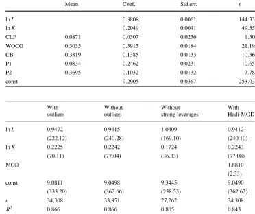
Table 2 OLS estimates of an
extended CDF with Bernoulli distributed regressors
Note:n=20,332;R2=0.846.
The regressors CLP
(company-level pact), WOCO (works council), CB (collective industry-wide bargaining), P1 (profits last year: very good) and P2 (profits last year: good) are dummies
Mean Coef. Std.err. t
lnL 0.8808 0.0061 144.33
lnK 0.2049 0.0041 49.55
CLP 0.0871 0.0307 0.0236 1.30
WOCO 0.3035 0.3915 0.0184 21.19
CB 0.3819 0.1385 0.0133 10.36
P1 0.0834 0.2462 0.0231 10.65
P2 0.3695 0.1032 0.0132 7.78
const 9.2905 0.0367 253.03
Table 3 OLS estimates of
CDFs with and without outliers,
t-values in parentheses; dependent variable: logarithm of sales—lnY
With outliers
Without outliers
Without strong leverages
With Hadi-MOD
lnL 0.9472 0.9415 1.0409 0.9412
(222.12) (240.28) (169.10) (240.10)
lnK 0.2225 0.2242 0.1724 0.2243
(70.11) (77.04) (36.33) (77.08)
MOD 1.8810
(2.33)
const 9.0811 9.0498 9.3445 9.0490
(333.20) (362.66) (238.53) (362.62)
n 34,308 33,851 27,262 34,308
R2 0.866 0.866 0.805 0.843
larger cluster-robust estimates of standard errors than that from the other methods.
An extended version of the Cobb-Douglas function in Table1 is presented in Table2. The latter estimates show smaller coefficients and smaller t-values of the input fac-tors labor and capital. The major intention of Table 2 is to demonstrate that also in this example there is—as main-tained in Sect.2.1.4—a clear relationship between D, the¯ mean of a dummy as independent variable, and the estimated standard errors. The nearerD¯ to 0.5 the smaller is the stan-dard error. The results in Table2 cannot be generalized in contrast to that in Table11because the standard error of a
dummy is not only determined by the mean. Each regressor has a specific influence on the dependent variable indepen-dent of the regressor’s variance.
Table 4 Confidence intervals (CI) of output elasticities of labor and
capital based on a Cobb-Douglas production function, estimated with and without outliers, Stoye’s confidence interval at partially identified parameters; dependent variable: logarithm of sales—lnY
CI with outliers
CI without outliers
Stoye CI ˆ
βlnL;u 0.9555 0.9492 0.9511
ˆ
βlnL;l 0.9388 0.9339 0.9376
ˆ
βlnK;u 0.2287 0.2299 0.2282
ˆ
βlnK;l 0.2162 0.2185 0.2184
βˆlnL 0.0167 0.0153 0.0135
βˆlnK 0.0125 0.0114 0.0098
under a wider definition of an outlier, e.g. if 3 is substituted by 2. The picture becomes also clearer if observations with high leverage are eliminated—see column 3. Coefficients and standard errors in column 1 and 3 reveal a clear dispar-ity for both input factors. This result is not unexpected but the consequence is ambiguous. Is column 1 or 3 preferable? If all observations with strong leverages are due to measure-ment errors the decision speaks in favor of the estimates in column 3. As no information is available to this question both estimates may be useful.
Column 4 extends the consideration to outliers follow-ing Hadi (1992).The squared difference between individual regressor values and the mean for all regressors—here lnL and lnK—is determined for each observation weighted by the estimated covariance matrix—see Sect.2.1.5. The deci-sion whether establishmenti is an outlier is now based on the Mahalanobis distance. MOD, the vector of multiple out-lier dummies (MODi=1 ifiis an outlier;=0 otherwise), is incorporated as an additional regressor. The estimates show that outliers have a significant effect on the output variable lnY. The coefficients and the t-values in column 2 and 4 are very similar. This is a hint that the outliers defined via
ˆ
u∗are mainly determined by large deviations of the regres-sor values. Fromuˆ∗ it is unclear whether the values of the dependent variable or the independent variables are respon-sible for the fact that an observation is an outlier.
As it is not obvious whether the outliers are due to mea-surement errors that should be eliminated or whether these are unusual but systematically induced observations that should be accounted for, parameters can only partially be identified. Therefore, in Table4confidence intervals are not only presented for the two extreme cases (column 1: all outliers are induced by specific events; column 2: all out-liers are due to random measurement errors). Additionally, in column 3 the confidence interval (CI) based on Stoye’s method is displayed. The results show that the lower and upper coefficient estimates of lnLby Stoye lies within the estimated coefficients in column 1 and 2. The upper coeffi-cient is nearer to that of column 2 and the lower is nearer
Table 5 Unconditional and conditional DiD estimates with
com-pany-level pact (CLP) effects; dependent variable: logarithm of sales—lnY
Unconditional Conditional
lnL 0.9423
(166.03)
lnK 0.2211
(53.37)
CLP 3.1152 0.0951
(35.91) (2.36)
D2009 0.0597 0.0216
(2.25) (1.54)
CLP∗D2009 −0.3029 0.0400
(−2.90) (0.84)
n 31,985 20,490
R2 0.101 0.841
Note:t-values in parentheses
to column 1. We do not find the same pattern for input fac-tor lnK. In this case Stoye’sβˆlnK;udeviates more from that in column 2 than in column 1. And forβˆlnK;l we find the opposite result. Stoye’s intervals (βˆlnL= ˆβlnL;u− ˆβlnL;l; βˆlnK= ˆβlnK;u− ˆβlnK;l) are shorter than that with or with-out with-outliers. In other words, the estimates are more precise.
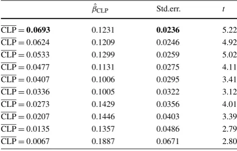
Table 6 Estimates of CDFs with CLP effects using matching
proce-dures; dependent variable: logarithm of sales—lnY
No matching MM NNM
lnL 0.9420 0.9362 0.9533
(166.03) (47.75) (63.32)
lnK 0.2212 0.1938 0.2007
(53.42) (15.12) (19.70)
CLP 0.1231 0.1928 0.0496
(5.22) (1.31) (1.46)
n 20,490 1,806 3,346
R2 0.840 0.838 0.849
Note: MM—Mahalanobis metric matching, NNM—nearest neighbor
matching,t-values in parentheses. Matching variables are profit situ-ation, year in which the establishment was founded, introduction of new products, further training, average working time, working time accounts, opening clause
Alternative methods to determine causal effects are matching procedures. These are suggested when there does not exist control over the assignment of treatment condi-tions, when in the basic equationy=Xβ+αD+uthe di-chotomous treatment variableDand the disturbance termu correlate, when the ignorable treatment assignment assump-tion is violated. In the example of the CDF it is quesassump-tioned that this condition is fulfilled for CLPs. As an alternative the Mahalanobis metric matching (MM) without propen-sity score and the nearest neighbor matching (NNM) with caliper are applied, presented in Table6, column 2 and 3, respectively. In the latter method non-replacement is used. That is, once a treated case is matched to a non-treated case, both cases are removed from the pool. The former method allows that one control case can be used as a match for sev-eral treated cases. Therefore, the total number of observa-tions in the nearest neighbor is larger than that in column 2. We find that the CLP effect on sales is insignificant in both cases but the CLP coefficient of MM estimates exceeds by far that of NNM. The estimates of the partial elasticities of production are very similar in the three estimates in Table6. The insignificance of the CLP effect confirms the result of column 2 of Table 5. If the DiD estimator of column 2 in Table5 is applied after matching the causal effect is—not unexpected—also insignificant. The probvalue is 0.182 if the MM procedure is used and 0.999 under the NNM proce-dure.
The previous estimates have demonstrated that company-level pacts (CLP) have no statistically significant influence on output. We cannot be sure that this result is also true for subgroups of firms. One way to test this is to conduct quan-tile estimates. As presented in Sect.2.2four methods can be applied to determine quantile treatment effects (QTE). The CLP effects on sales can be found in Table 7 where the results of five quantiles (q =0.1,0.3,0.5,0.7,0.9) are
presented. In contrast to the previous estimations most CLP effects are significant in the columns 1–4 of Table7. Firpo considers the simplest case without control variables under the assumption that the adoption of a company-level pact is exogenous. The estimated coefficients in column 1 (F) seem oversized. The same follows from the Frölich-Melly approach, where CLP is instrumented by a short work time dummy (column 3—F-M). Other available instruments like opening clauses, collective bargaining, works councils or re-search and development within the firm do not evidently change the results. One reason for the overestimated coef-ficients can be neglected determinants of the output that cor-relate with CLP. Estimates of column 2 (K-B) and 4 (A-A-I) support this hypothesis.
From the view of expected CLP coefficients the con-ventional quantile estimator, the Koenker-Bassett approach, with lnL and lnK as regressors seems best. However, the ranking of the size of the coefficients within column 2 seems unexpected. The smaller the quantile the larger is the es-timated coefficient. This could mean that CLPs are advan-tageous for small firms. However, it is possible that small firms with advantages in productivity due to CLPs have rela-tive high costs to adopt a CLP. In this case the higher propen-sity of large firms to introduce a CLP is consistent with higher productivity of small firms.
The coefficients of the Abadie-Angrist-Imbens approach, a combination of Frölich-Melly’s and Koenker-Bassett’s model, are also large but not so large as in column 1 and 3.
Table 7 Quantile estimates of CLP effects; dependent variable: logarithm of sales—lnY
Quantile F K-B F-M A-A-I MM+K-B MM+A-A-I
q=0.1 2.9957 0.2236 5.3012 1.2092 −0.1064 0.9776
(38.94) (6.76) (20.42) (3.10) (−0.87) (1.06)
q=0.3 3.3242 0.1836 5.8227 1.1615 0.0715 0.7140
(54.67) (7.15) (23.67) (3.11) (0.46) (0.62)
q=0.5 3.1325 0.1526 6.3549 1.2000 0.1793 0.6736
(54.19) (6.31) (24.58) (2.57) (1.09) (1.37)
q=0.7 2.9312 0.1036 6.8703 1.2479 0.2270 0.8072
(56.91) (4.07) (26.14) (2.09) (1.54) (2.18)
q=0.9 2.3203 −0.0176 7.8119 1.6549 0.4523 1.4242
(34.18) (−0.37) (20.12) (1.36) (3.36) (2.92)
n 31,985 20,490 20,909 13,496 1,806 1,206
Note: F—Firpo; K-B—Koenker/Bassett; F-M—Frölich/Melly; A-A-I—Abadie/Angrist/Imbens, MM—Mahalanobis metric matching, control
variables are lnLand lnK,t-values in parentheses
Fig. 1 Regression discontinuity of CLP probability
The final discussed treatment method in Sect.2.2is the regression discontinuity (RD) design. This approach ex-ploits information of the rules determining treatment. The probability of receiving a treatment is a discontinuous func-tion of one or more variables where treatment is triggered by an administrative definition or an organizational rule.
In a first example using a sharp RD design it is analyzed whether at an estimated probability of 0.5 that a company-level pact (CLP) exists a structural break on logarithm of output (lnY) is evident. For this purpose a probit model is estimated with profit situation, working-time account, total wages per year and works council as determinants of CLP. All coefficients are significantly different from zero—not in the tables. The estimated probability Pr(CLP)is then plotted against lnY based on a fractional polynomial model over the entire range (0<Pr(CLP) <1) and on two linear models split into Pr(CLP) <=0.5 and Pr(CLP) >0.5. The graphs are presented in Fig.1.
A structural break seems evident. Two problems have to be checked: First, is the break due to a nonlinear shape, and second, is the break significant? The answer to the first ques-tion is yes, because the shape over the range 0<Pr(CLP) < 1 is obviously nonlinear when a fractional polynomial is assumed. The answer to the second question is given by a t-test—cf. Sect.2.2—based on
y =γ0+γ1D_Pr(CLP)+γ2
Pr(CLP)−Pr(CLP) +γ3D_Pr(CLP)·
Pr(CLP)−Pr(CLP)+u =:γ0+γ1D_Pr(CLP)+γ2cPr(CLP)
+γ3D_Pr(CLP)·cPr(CLP)+u,
where
D_Pr(CLP)=
1 if Pr(CLP)≤0.5 0 otherwise.
The null that there is no break has to be rejected (γˆ1= −3.96;t= −6.87; probvalue=0.000) as can be seen in Ta-ble8.
The estimates in Table8cannot tell us whether the out-put jump in Pr(CLP)=0.5 is a general phenomenon or whether the Great Recession in 2008/09 is responsible. To test this the combined method of RD and DiD—derived in Sect.2.2—is employed and the results are presented in Table 9. The estimates show that the output jump does not significantly change between 2006/2007 and 2008/2010. The influence ofD_Pr(CLP)·T and that ofD_Pr(CLP)· cPr(CLP)·T on lnY is insignificant. Therefore, we con-clude that the break is of general nature.
Table 8 Testing for structural
break of CLP effects between Pr(CLP)≤0.5 and
Pr(CLP) >0.5
Coef. Std.err. t P >|t|
D_Pr(CLP) −3.9608 0.5765 −6.87 0.000
cPr(CLP) 4.3413 0.8390 5.17 0.000
D_Pr(CLP)·cPr(CLP) 11.3838 0.8437 13.49 0.000
const 18.4375 0.5764 31.99 0.000
Table 9 Testing for differences
in structural break of CLP effects between Pr(CLP)≤0.5 and Pr(CLP) >0.5 in 2006/07 and 2008/10
Coef. Std.err. t P >|t|
T 0.0130 1.3118 0.01 0.992
D_Pr(CLP) −4.1045 1.1191 −3.67 0.000
cPr(CLP) 3.9314 1.6795 2.34 0.019
D_Pr(CLP)·cPr(CLP) 11.6383 1.6884 6.89 0.000
D_Pr(CLP)·T 0.0392 1.3119 0.03 0.976
cPr(CLP)·T 0.2801 1.9520 0.14 0.886
D_CLP·cPr(CLP)·T −0.0662 1.9623 −0.03 0.973
const 18.5422 1.1190 16.57 0.000
Fig. 2 Regression discontinuity of small firms
as such that have less than 10 employees and until 1 mil-lion Euro sales per year. The analogous definition of middle-size firms is less than 500 employees and until 50 million Euro sales per year. A sharp regression discontinuity de-sign is applied to test whether the first and the second part of the definition are consistent. In other words, based on a Cobb-Douglas production function with only one input fac-tor, the number of employees, it is tested whether there exists a structural break for small firms between 9 and 10 employ-ees at a 1 million sales border. We find for small firms in Fig.2that there seems to be a sales break around 1 million Euro per year.
The t-test analogously to the first example yields weak significance (γˆ1 = −13.8667; t = −1.61; probvalue = 0.107). The same procedure for middle-size firms—see Fig.3—leads to following results.
Fig. 3 Regression discontinuity of middle-size firms
Apparently, there exists a break. However, the first part of the definition of middle-size firms from the Institut für Mittelstandsforschung is not compatible with the second part. The break of sales at 500 employees is not 50 million Euro per year but around 150 million Euro. Furthermore, the visual result might be due to a nonlinear relationship as the fractional polynomial estimation over the entire range suggests. Thet-test does not reject the null (γˆ1= −8977; t= −0.54; probvalue=0.588). The conclusion from Fig.2 and3is that the graphical representation without the poly-nomial shape as comparison course and without testing for a structural break can lead to a misinterpretation.
(a)
(b)
Fig. 4 (a) Regression discontinuity of ln(sales). (b) Regression
dis-continuity of treatment CLP
Table 10 Fuzzy regression discontinuity between East and West
Ger-man federal states (GFS)—Wald test for structural break of compa-ny-level pact (CLP) effects on sales; jump at GFS>0; dependent vari-able: logarithm of sales—lnY
Variable Coef. Std.err. z
lnYjump −0.8749 0.1234 −7.09
CLP jump −0.0571 0.0138 −4.13
Wald estimator 15.3165 3.5703 4.29
Note: GFS= −10 Berlin(West); −9 Schleswig-Holstein;−8
Ham-burg; −7 Lower Saxony;−6 Bremen; −5 North Rhine-Westphalia; −4 Hesse; −3 Rhineland-Palatinate; −2 Baden-Württemberg; −1 Bavaria; 0 Saarland; 1 Berlin(Ost); 2 Brandenburg; 3 Mecklenburg-West Pomerania; 4 Saxony; 5 Saxony-Anhalt; 6 Thuringia
the disparities in the level of sales per year and the latter those of Pr(CLP)—here measured by the relative frequency of firms with a CLP to all firms in a German federal state.
Although clear differences are detected for both charac-teristics (lnY,Pr(CLP)) we cannot be sure that these dis-parities are significant and whether the CLP effects are
smaller or larger in West Germany. This is checked by a Wald test in Table10. We find that the CLP effects on lnY (−0.8749/−0.0571=15.3165) are significantly higher in the West German federal states (z=4.29). When the inter-pretation is focussed on the dummy “East Germany” as an instrument of a dummy “CLP” we should note that the for-mer is not a proper instrument because the output lnYdiffers between East and West Germany independent of a CLP.
4 Summary
Many reasons like heteroskedasticity, clustering, basic prob-ability of qualitative regressors, outliers and only partially identified parameters may be responsible that estimated standard errors based on classical methods are biased. Ap-plications show that the estimates under suggested modifi-cations do not always deviate so much from that of the clas-sical methods.
The development of new procedures is ongoing. Espe-cially, the field of treatment methods were extended. It is not always obvious which method is preferable to determine the causal effect. As the results evidently differ it is nec-essary to develop a framework that helps to decide which method is most appropriated under typically situations. We observe a tendency away from the estimation of average ef-fects. The focus is shifted to distribution topics. Quantile analysis helps to investigate differences between subgroups of the population. This is important because economic mea-sures have not the same influence on heterogeneous estab-lishments and individuals. A combination of quantile re-gression with matching procedure can improve the determi-nation of the causal effects. Further combidetermi-nations of treat-ment methods seem helpful. Difference-in-differences esti-mates should be linked with matching procedures and re-gression discontinuity designs. And also rere-gression discon-tinuity split to quantiles can lead to new insights.
Executive summary
counterproductive for policy measures? In order to avoid this, the practitioner has to be familiarwith the wide range of existing methods for the empirical investigations. The user has to know the assumptions of the methods and whether the application allows adequate conclusions at given infor-mation. It is necessary to check the robustness of the results by alternative methods and specifications.
This paper presents a selective review of econometric methods and demonstrates by applications that the meth-ods work. In the first part, methodological problems to standard errors and treatment effects are discussed. First, heteroskedasticity- and cluster-robust estimates are pre-sented. Second, peculiarities of Bernoulli distributed regres-sors, outliers and only partially identified parameters are revealed. Approaches to the improvement of standard error estimates under heteroskedasticity differ in the weighting of residuals. Other procedures use the estimated disturbances in order to create a larger number of artificial samples, to obtain better estimates. And again others use nonlinear in-formation. Cluster robust estimates try to solve the Moul-ton problem. Too low standard errors between observations within clusters are adjusted. This objective is only partially successful. We should be cautious if we compare the effects of dummy variables on an endogenous variable, because the more the mean of dummies deviates from 0.5 the higher are the standard errors. Outliers, i.e. unusual observations that are due to systematic measurement errors or extraordinary events may have enormous influence on the estimates. The suggested approaches to detect outliers vary relating to the measurement concept and do not necessarily demonstrate whether outliers should be accounted for in the empirical analysis. New methods for partially identified parameters may be helpful in this context. Under uncertainty the degree of precision, whether outliers should be eliminated, can be increased.
Four principles to estimate causal effects are in the focus: difference-in-differences (DiD) estimators, matching proce-dures, quantile treatment effects (QTE) analysis and regres-sion discontinuity design. The DiD models distinguish be-tween conditional and unconditional approaches. The range of the popular matching procedures is wide and the meth-ods evidently differ. They aim to find statistical twins, to ho-mogenize the characteristics of observations from the treat-ment and the control group. Until now, the application of QTE analysis is relatively rare in practice. Four types of models are important in this context. The user has to de-cide whether the treatment variable is exogenous or endoge-nous and whether additional control variables are incorpo-rated or not. Regression discontinuity (RD) designs separate between sharp and fuzzy RD methods. It is distinguished whether an observation is assigned to the treatment or to the control group directly by an observable continuous variable or indirectly via the probability and the mean of treatment, respectively, conditional on this variable.
In the second part of the paper the different methods are applied to estimates of Cobb-Douglas production functions using IAB establishment panel data. Some heteroskedasticity-consistent estimates show similar results while cluster-robust estimates differ strongly. Dummy variables as re-gressors with a mean near 0.5 reveal as expected smaller variances of the coefficient estimators than others. Not all outliers have a strong effect on the significance. Methods of partially identified parameters demonstrate more efficient estimates than traditional procedures.
The four discussed treatment effects methods are applied to the question whether company-level pacts have a signif-icant effect on the production output. Unconditional DiD estimators and estimates without matching display signif-icantly positive effects. In contrast to this result we can-not find the same if conditional DiD or matching estimates based on the Mahalanobis metric are applied. This outcome has more precisely formulated under quantile regression. The higher the quantile the more is the tendency to posi-tive and significant effects. Sharp regression discontinuity estimates display a jump at the probability 0.5 that an es-tablishment has a company-level pact. No specific influence can be detected during the Great Recession. Fuzzy regres-sion discontinuity estimates reveal that the output effect of company-level pacts is significantly lower in East than in West Germany. A combined application of the four prin-ciples determining treatment effects lead to some interest-ing new insights. We determine joint DiD and matchinterest-ing es-timates as well as that ofthe former together with regres-sions discontinuity designs. Finally, matching is interrelated to quantile regression.
Kurzfassung