Forestry & Natural-Resource Sciences Last Correction: Aug. 5, 2010
THE ROLE OF MISCLASSIFICATION IN ESTIMATING
PROPORTIONS AND AN ESTIMATOR OF MISCLASSIFICATION
PROBABILITY
Patrick L Zimmerman
1,2, Greg C Liknes
2,
1School of Statistics, University of Minnesota - Twin Cities, Minneapolis, MN 2USDA Forest Service, Northern Research Station, St. Paul, MN
Abstract.Dot grids are often used to estimate the proportion of land cover belonging to some class in an
aerial photograph. Interpreter misclassification is an often-ignored source of error in dot-grid sampling that has the potential to significantly bias proportion estimates. For the case when the true class of items is unknown, we present a maximum-likelihood estimator of misclassification probability based on agreement between two interpreters. Two of the assumptions underlying the estimator are: (i) the probability that an interpreter makes a misclassification is constant, (ii) both interpreters have the same probability of misclassification. Simulation results suggest the estimator has acceptable performance when (ii) does not hold. This estimator can be used to investigate whether bias due to misclassification has exceeded a threshold, or to correct bias due misclassification.
Keywords:Dot grid, remote sensing, image interpretation, misclassification
1
Introduction
Aerial photography has been used extensively as a tool in natural resource assessments in a variety of ways, par-ticularly in forestry. For example, aerial photography has been used to assess the damage from pests such as mountain pine beetle (White et al. 1983) and eastern spruce budworm (Munson et al. 1985). Hansen (1985) used linear transect sampling with airphotos to inven-tory wooded strips in Kansas. More recently, Frescino et al. (2006) used aerial imagery to assess forest resources in Nevada. A dataset of forest canopy density across the United States was developed by modeling the relation-ship between interpreted airphotos and Landsat satellite imagery (Huang et al. 2001).
For decades, airphotos played a vital role in forest in-ventory programs (Loetsch and Haller 1964). The USDA Forest Service Forest Inventory and Analysis program photo-classified nearly 200,000 1-acre photo points into forest land, unproductive forest, nonforest, and water categories in support of the 1983 Wisconsin (USA) in-ventory (Spencer et al. 1988). Forest inin-ventory appli-cations of airphotos include area estimation, stratifica-tion, photo sampling, and map creation. With regard to photo sampling, aerial photographs may be used in con-junction with dot grids to estimate proportions of a
fea-! ! ! ! ! ! ! ! ! ! ! ! ! ! ! ! ! ! ! ! ! ! ! ! ! ! ! ! ! ! ! ! ! ! ! ! ! ! ! ! ! ! ! ! ! ! ! ! ! ! ! ! ! ! ! ! ! ! ! ! ! ! ! ! ! ! ! ! ! ! ! ! ! ! ! ! ! ! ! ! ! ! ! ! ! ! ! ! ! ! ! ! ! ! ! ! ! ! ! !
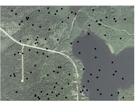
Figure 1: a sample dot grid with randomly located dots.
ture of interest. Historically, an interpreter would place a transparent overlay with a regular or systematic dot grid on top of an airphoto and assign dots to a category of interest (e.g., tree/no tree or damaged/not damaged). Proportions are simply the relative counts in each of the categories divided by the total dot count. Dot grid meth-ods have moved forward into the digital age, and tools have been developed for use with digital aerial imagery
Copyright c2010 Publisher of the International Journal ofMathematical and Computational Forestry & Natural-Resource Sciences
(e.g., Clark et al. 2004, Lister et al. 2009) (Figure 1). In addition to digital tools, natural resource practition-ers now have access to an ever-increasing collection of high-resolution imagery from the United States. The USDA’s National Agriculture Imagery Program (NAIP) has been collecting aerial imagery since 2003. A few states are flown over and photographed each year, with an approximate return interval of three years. Many states have also acquired their own resource photogra-phy, such as the New York State Digital Orthophoto Program (NYSDOP) imagery, Pennsylvania’s PAMAP imagery, and the New Jersey Department of Environ-mental Protection (NJDEP) imagery.
While considerable work is being done in the area of image segmentation and automated feature extrac-tion for natural resource inventory and monitoring (e.g., Chubey et al. 2006, Smith et al. 2008, Laliberte et al. 2004), dot grids still represent an efficient method for estimating proportions over large areas. The topics of sample size (Gering and Bailey 1984) and sampling er-ror (Bonnor 1974) for dot grids have been given con-siderable attention. However, the error associated with proportions estimated from dot grids arises from two sources: sampling error and misclassification of individ-ual dots. Considering only the binary case (tree/no tree, damage/no damage), we discuss a mathematical model of proportion estimates that includes misclassification (Section 2), and then derive and discuss a possible es-timator of misclassification probability as a function of interpreter agreement (Section 3). Along with sampling error, this estimate should provide a more realistic esti-mate of total error in proportions as derived from inter-preted data. While application to dot grids is intended, the model applies more generically to any data an inter-preter assigns to one of two classes.
2
The impact of misclassification
2.1 A mathematical model for misclassification The effects of misclassification on a sample estimate of a proportion have been described by Bross (1954). Sup-pose that an estimate of the proportion of items in a population that fall into some class C is desired, and thatpis the proportion of items inC in the population with the rest being in class N. Suppose furthermore that there is aθprobability of misclassification for each item (in either class). Now, a sample of sizenis drawn, and the number of items,X, classified asCare counted. A typical estimator of p, X/n (denoted ¯Xn), will be biased. Its expected value is changed due to misclassifi-cation such that
E( ¯Xn) =p−2pθ+θ
This implies that the bias of the estimate is
E( ¯Xn)−p=−2pθ+θ (1)
Despite its bias, ¯Xn still follows a binomial distribu-tion.
To give an idea of the magnitude of this bias in a con-crete scenario, suppose that a photo interpreter classifies dots in a dot grid as either falling on tree canopy (class
C) or not (classN), and misclassifies dots in both classes 5% of the time. In the notation of the previous section,
θ = 0.05. If this were the case, a population with a true proportion inC of 20% would haveE( ¯Xn) = 23% - i.e., a 3% bias - and a population with 10% proportion would haveE( ¯Xn) = 14%. As these examples suggest, the bias is drawing the estimator towards 50% because there are more dots truly in classN, and therefore more opportunities to misclassify classN dots as classC. This example implies that if many proportions are estimated with some misclassification each estimate would be bi-ased toward 50% (from either direction). Importantly, this is not a problem that would be “washed out” across many populations. Whereas sampling error decreases as a sample size increases, bias due to misclassification will remain.
It should be noted that this model assumes that the misclassification rate is identical for items in both classes. In fact, Bross (1954) presents this model for the more general case where the probability of misclassify-ing items in class C is not necessarily the same as that of misclassifying items in class N. The possibility of developing the current work in this more general frame-work is discussed later. Also, note that misclassification is not the only potential source of bias. For example, systematic sampling can result in a bias.
2.2 What can be done about bias due to mis-classification? There is often no way to collect the in-formation necessary to directly estimate misclassifica-tion probabilities. We may never know the correctness of an interpreter’s classifications, only his/her agreement with those of another (fallible) interpreter. For example, in the case of photo interpretation studies, it is likely in-feasible to verify the correctness of classified dot grids with in situ observations. To summarize the problem with proportion estimates where misclassification prob-abilities are non-zero but unknown, the estimates are biased to an unknown and possibly large extent.
0.0 0.2
0.4 0.6
0.8
1.0 −1.0 −0.5
0.0 0.5
1.0
0.0 0.2 0.4 0.6 0.8 1.0
θ
ρ α
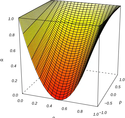
Figure 2: Interpreter agreement (α) as a function of mis-classification probability (θ) and the correctness corre-lation (ρ).
Result. Let αbe the probability of agreement between two interpreters, letθdenote the misclassification proba-bility, and letρbe the correlation between the correctness of classifications made by the two interpreters (this value is discussed below). Then,
α=θ2+ 2ρθ(1−θ) + (1−θ)2 (2) This result is fully developed in the appendix, but for now, a little explaining is in order, and a graphical depiction of the relationship is presented in Figure 2. This relationship states that agreement is a quadratic function of misclassification probability. If the two in-terpreters are either always right or always wrong, they will always agree. What happens in every other case depends on the correctness correlation, ρ. If the inter-preters tend to misclassify the same items, ρ will be positive. If one interpreter is more likely to correctly classify the items misclassified by the other interpreter,
ρwill be negative. In a case where all interpreters have received the same training and successfully follow the same procedure in classifying items, it is expected that
ρwill be non-negative. The two interpreters may have a difficult time classifying certain types of items, and the interpreters should be using the same strategies to classify items that are not immediately obvious. Note that, ifρis zero, knowing that the first interpreter mis-classified an item offers no information about whether or not the second interpreter misclassified that item. Using the above relationship, we can use observed agreement between interpreters to say something useful about
mis-classification, and, subsequently, the bias of estimated proportions.
3
Estimating a misclassification
prob-ability
3.1 Statement of the estimator Suppose that two fallible interpreters classify items as belonging to one of two classes, but that the true class of the items is unknown. With a few assumptions, it is possible to get an estimate of their misclassification probability based on paired classifications made by the interpreters, and to calculate the asymptotic variance of this estimate. Note that the individual paired classifications made by the interpreters must be known for each item, and not just the total number of items in the population classified as belonging to each class by the interpreters. A formal statement of the following theorem and a proof are given in the appendix. Also, the more general case whereρ∈
(−1,1) is considered in the appendix.
Theorem. Suppose that two interpreters classify n different items, and that A1,A2, . . . ,An are observed where Ai = 1 if the interpreters agree on item i, and
Ai = 0 otherwise, for i = 1, . . . , n. Suppose also that the following assumptions hold,
(A1) the classifications for each item made by an inter-preter are independent and have the same misclas-sification probability.
(A2) the classifications made by both interpreters have aθ probability of misclassification.
(A3) θ < 12. (A4) ρ= 0.
then, if we define A¯n= 1
n n
i=1Ai, ˆ
θ= 1 2 −
2 ¯An−1
4 (3)
is the maximum likelihood estimator of θ, and is nor-mally distributed with mean θ and variance 4αn(1(2−α−α)1) as n→ ∞. If an estimate of the asymptotic variance ofθˆis desired, it is recommended that the maximum likelihood estimate ofα,A¯n, be used in place of α.
uses the same procedure to classify each dot, it seems reasonable to believe that the misclassification probabil-ity for an item will depend only on characteristics of that item, and not, for example, on how difficult to classify the previous item was or how many items the interpreter has classified. The assumption of a constant probability could be unrealistic, though. For example, if interpreters are classifying dots from a dot grid as landing on tree cover or not, misclassification probabilities could differ depending on where a dot is located in the image. It may be more likely that misclassification will occur in sparse forest than in dense forest or an open area. (A2) is not very realistic, but simulation suggests that, if the two interpreters have different misclassification probabil-ities, ˆθ is an estimator of their average misclassification probability. These results are presented shortly. (A3) only requires that the interpreters are classifying at least half of the items correctly. (A4) seems problematic at first. However, recall the scenario described above un-der which ρwould be expected to be positive (Section 2.2): the two interpreters are more likely to misclassify some items than others. Given(A1), this cannot occur, and, as long as the interpreters are working separately, it is difficult to imagine another scenario under whichρ
would be non-zero.
3.2.1 Simulation study of (A2) Assumption(A2) states that both interpreters have the same misclassifi-cation probability. This assumption will certainly never be exactly true. Therefore, a simulation study was con-ducted to determine the behavior of ˆθunder a variety of scenarios.
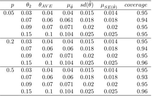
First, a population was defined to have either 5%, 20%, or 50% of the items in categoryC. Classifications of these items by two fallible interpreters were simulated with a correctness correlation of zero. The first inter-preter always had a 5% misclassification while the second interpreter had either a 3%, 7%, 9%, or 15% misclassifi-cation probability. Then, 10000 samples of size 100 were drawn from this population.
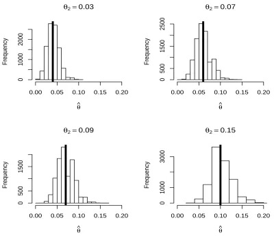
95% confidence intervals were calculated in each sam-ple. Figure 3 and Figure 4 present histograms of ˆθ and the estimated SE(ˆθ), respectively, from the population with 50% of the items in classC. Note that, in Figure 4, the sample standard deviations of the estimates are de-picted. The sample standard deviation is measuring the variation of ˆθ that actually occurred in the simulation. Thus, it can be considered a target value for estimated standard errors. Table 1 shows numerical results from each population.
This simulation study suggests that, when the misclas-sification probabilities of two interpreters differs, ˆθ be-haves approximately as if it were estimating the misclas-sification probability of two other interpreters who both
Table 1: Simulation results. p is the true proportion of items in classC; θ2 is the misclassification probabil-ity of the second interpreter (θ1 = 0.05 always); θAV E is the average misclassification probability between the two interpreters; μθˆ is the mean observed ˆθ; sd(ˆθ) is the sample standard deviation of the simulated misclas-sificaion probability estimates; μSE( ˆθ) is the mean ob-served SE(ˆθ); coverage is the proportion of times that a 95%CI covered θAV E.
p θ2 θAV E μθˆ sd(ˆθ) μSE( ˆθ) coverage
0.05 0.03 0.04 0.04 0.015 0.014 0.95
0.07 0.06 0.061 0.018 0.018 0.94
0.09 0.07 0.071 0.02 0.02 0.95
0.15 0.1 0.104 0.025 0.025 0.95
0.2 0.03 0.04 0.04 0.015 0.014 0.95
0.07 0.06 0.06 0.018 0.018 0.94
0.09 0.07 0.071 0.02 0.02 0.95
0.15 0.1 0.104 0.025 0.025 0.96
0.5 0.03 0.04 0.04 0.015 0.014 0.95
0.07 0.06 0.06 0.018 0.018 0.93
0.09 0.07 0.071 0.02 0.02 0.95
0.15 0.1 0.104 0.025 0.025 0.96
had the average misclassification of the first two. Esti-mates tend to be slightly inflated (less than 1%) when the second interpreter has a 15% misclassification proba-bility. Note also that, although the theoretical standard error,SE(ˆθ), is asymptotic (its behavior is known only asn→ ∞), the observed coverage probabilities suggest that the estimated standard error is performing well at this sample size.
4
Discussion
4.1 Usefulness of θˆ Any study that produces pro-portion estimates based on fallible classifications and states the precision of its estimates should try to account for misclassification. If misclassification probabilities are not known and proportion estimates are reported as if they were unbiased, they have the potential to be very misleading. Such a study could utilize ˆθin at least two different ways.
θ2=0.03
θ
^
Frequency
0.00 0.05 0.10 0.15 0.20
0
1000
2000
θ2=0.07
θ
^
Frequency
0.00 0.05 0.10 0.15 0.20
0
500
1500
2500
θ2=0.09
θ
^
Frequency
0.00 0.05 0.10 0.15 0.20
0
500
1500
θ2=0.15
θ
^
Frequency
0.00 0.05 0.10 0.15 0.20
0
1000
3000
Figure 3: Histograms of misclassification estimates, ˆθ. θ1 = 0.05 andp= 0.5 in each histogram. The thick vertical line represents the average misclassification rate.
from a proportion estimate, that estimate’s bias due to misclassification would be corrected.
The largest problem with using ˆθ in either of these ways is the requirement that the misclassification prob-ability for each item is identical. A substantial deviation from this assumption would likely be associated with a deviation from the assumption thatρis equal to zero.
4.2 Future work In this paper, the case was consid-ered where the probability of misclassification was con-stant across items classified by an interpreter, which may not be a realistic scenario. It may be helpful to consider two ways in which this assumption may be broken: (i) classification may have a difficulty level that varies for each item, and (ii) the probability of misclassification of items in class C may be different from those in class
N. For (i), a more realistic model could be developed if a hierarchical model is used. Specifically, the
proba-bility of misclassification itself could perhaps be treated as a random variable that is bounded between zero and one. The target value for estimation would then be the mean misclassification probability. The case (ii) may be more difficult if it is necessary to estimate the misclassifi-cation probability for both classes. This difficulty arises because, for any given classification, the true class of the item is unknown. Hence, it would be unknown whether agreement on this classification was providing informa-tion about the misclassificainforma-tion probability of items in classC or items in classN.
5
Acknowledgments
θ2=0.03
SE(θ^)
Frequency
0.00 0.01 0.02 0.03 0.04
0
1000
2000
θ2=0.07
SE(θ^)
Frequency
0.00 0.01 0.02 0.03 0.04
0
500
1500
2500
θ2=0.09
SE(θ^)
Frequency
0.00 0.01 0.02 0.03 0.04
0
500
1500
θ2=0.15
SE(θ^)
Frequency
0.00 0.01 0.02 0.03 0.04
0
1000
2000
3000
Figure 4: Histograms of the standard error of misclassification estimates,SE(ˆθ). θ1= 0.05 andp= 0.5 in each his-togram. The thick vertical line represents the sample standard deviation of the simulated misclassification probability estimates.
References
Bonnor, G.M. 1974. The error of area estimates from dot grids. Can. J. For. Res. 5(10): 10-17.
Bross, I. 1954. Misclassification in 2 X 2 tables. Biomet-rics 10(4): 478-486.
Casella, G. and R.L. Berger. 2002. Statistical Inference, 2nd ed. Duxbury. 243 p.
Clark, J.T., M.V. Finco, R. Warbington, and B. Schwind. 2004. Digital Mylar: A tool to attribute vegetation polygon features over high-resolution imagery. Available online at http://www.fs.fed.us/r5/rsl/publications/. Last accessed Jan. 20, 2010.
Chubey, M.S., S.E. Franklin, and M.A. Wulder. 2006. Object-based analysis of Ikonos-2 imagery for
extrac-tion of forest inventory parameters. Photogrammetric Engineering & Remote Sensing 72(4): 383-394.
Frescino, T.S., G.G. Moisen, K.A. Megown, V.J. Nelson, E.A. Freeman, P.L. Patterson, M. Finco, K. Brewer, and J. Menlove. 2009. Nevada Photo-Based Inventory Pilot (NPIP) photo sampling procedures. USDA For. Serv. Gen. Tech. Rep. RMRS-222. 30 p.
Gering, L.R. and R.L Bailey. 1984. Optimum dot-grid density for area estimation with aerial photographs. Journal of Forestry 82(7): 428-431.
Hansen, M. 1985. Line intersect sampling of wooded strips. Forest Science. 31(2): 282-288.
large areas. [CD-ROM] Disc 1 in Proc. of the Third In-ternational Conference on Geospatial Information in Agriculture and Forestry.
Laliberte, A.S., A. Rango, K.M. Havstad, J.F. Paris, R.F. Beck, R. McNeely, and A.L. Gonzalez. 2004. Object-oriented image analysis for mapping shrub en-croachment from 1937 to 2003 in southern New Mex-ico. Remote Sensing of Environment 93(1-2): 198-210.
Loetsch, F. and K.E. Haller. 1964. Forest Inventory Volume 1: Statistics of Forest Inventory and Infor-mation from Aerial Photographs. Bayerischer Land-wirtschaftsverlag GmbH. Munich, Germany.
Lister, A., T. Lister, and J.A. Doyle. 2009. Use of a sple photointerpretation method with free, online im-agery to assess landscape fragmentation. [CD-ROM] from Proc., 2009 Society of American Foresters na-tional convention, Opportunities in a forested world.
Munson, A.S., W.B. White, R.J. Myhre, and W.H. Hoskins. 1985. Evaluation of three survey methods for determining Spruce-Fir mortality caused by Eastern Spruce Budworm. Forest Pest Management Methods Application Group Report. 85-2. 18 p.
Smith, A.M.S., E.K. Strand, M.S. Caiti, D.B. Hann, S.R. Garrity, M.J. Falkowski, and J.S. Evans. 2008. Production of vegetation spatial-structure maps by per-object analysis of juniper encroachment in multi-temporal aerial photographs. Can. J. Remote Sensing 34(Suppl. 2): S1-S18.
Spencer, J.S., W.B. Smith, J.T. Hahn, and G.K. Raile. 1988. Wisconsin’s fourth forest inventory, 1983. Re-source Bulletin NC-107. St. Paul, MN: U.S. Dept. of Agriculture, Forest Service, North Central Forest Ex-periment Station.
White, W.B, W.E. Bousfield, and R.W. Young. 1983. A survey procedure to inventory ponderosa and lodge-pole pine mortality caused by the mountain pine bee-tle. Forest Service, Washington, D.C.
APPENDICES
More formal notation will be used in the Appendix in order show results concisely. Also, results will be derived for the more general condition where ρ∈(−1,1). The theorem from the body of the paper considers the special case whereρ= 0.
A
Relationship
between
agreement,
misclassification,
and
conditional
correlation
Result. Suppose that X1 and X2 are binary random
variables, such that P(X1 = 1) = P(X2 = 1) = 1−θ. Also, suppose that P(X1 = X2) = α and that Cor(X1,X2) =ρ. Then,
α=θ2+ 2ρθ(1−θ) + (1−θ)2 (3) Proof. Note that, for any random eventA,
P(A) = E(I(A))
Then,
α= P(X1= 1∩X2= 1) + P(X1= 0∩X2= 0) = E(I(X1= 1)I(X2= 1)) + E(I(X1= 0)I(X2= 0)) = E(X1X2) + E(I(X1= 0)I(X2= 0))
Now,
E(X1X2) = Cov(X1,X2) + E(X1)E(X2) and
Cov(X1,X2) =ρ
V(X1)V(X2)
Now, note that E(Xi) = 1−θ and V(Xi) =θ(1−θ) for
i= 1,2. Thus,
E(X1X2) =ρθ(1−θ) + (1−θ)2 Then,
E(I(X1= 0)I(X2= 0)) = Cov(I(X1= 0),I(X2= 0)) + E(I(X1= 0))E(I(X2= 0)) and since E(I(Xi= 0)) =θand V(I(Xi= 0)) =θ(1−θ) fori= 1,2, we see that
E(I(X1= 0)I(X2= 0)) =δθ(1−θ) +θ2
where δ is the correlation between the incorrectness of X1 and X2. At this point, all that remains is to show thatρ=δ. Note that, if
Cov(X1,X2) = Cov(I(X1= 0),I(X2 = 0)) then,ρ=δ. So,
Cov(X1,X2) = Cov(1−I(X1= 0),1−I(X2= 0)) = Cov(−I(X1= 0),−I(X2= 0)) = Cov(I(X1= 0),I(X2= 0))
B
Derivation of the estimator
Theorem. LetX11, . . . ,Xn1andX12, . . . ,Xn2be
ran-dom variables such that Xij represents the correctness interpreter i’s classification of the jth item. Denote P(Xij = 0) =θij fori= 1, . . . , n and j = 1,2. Finally, set Ai= 1where Xi1=Xi2and Ai= 0otherwise, and
denote αi = P(Ai = 1)for i= 1, . . . , n. Now, suppose the following assumptions are met:
(A1) (X11,X12), . . . ,(Xn1,Xn2) are independent and
θ1j=. . .=θnj=θj whenj = 1or2.
(A2) θ1=θ2=θ.
(A3) θ < 12.
Then, if we denote αˆ= n1ni=1Ai,
ˆ
θ= 1 2−
2 ˆα−1−ρ
4(1−ρ) (4)
is the maximum likelihood estimator of θ, and is normally distributed with mean θ and variance
α(1−α)
4n(2α−1−ρ)(1−ρ) as n → ∞ where Cor(Xi1,Xi2) = ρ
fori= 1, . . . , n.
Note: if an estimate of the asymptotic variance ofθˆis desired, it is recommended that the maximum likelihood estimate of α, ¯An,be used in place ofα.
Proof. This proof will proceed in two parts. Part 1 explores the relationship between θ, α, and ρ. In Part 2, the properties of ˆαand ˆθwill be derived.
Part 1. Letρbe defined as above, and apply(A1) and(A2). Then, the previous result supplies the follow-ing startfollow-ing point,
α=αi
=θ2+ 2ρθ(1−θ) + (1−θ)2 =θ(1−θ)(2ρ−2) + 1
α−1
2(ρ−1) =θ(1−θ)
Recognizing a quadratic function of θ, we complete the square and write
(θ−1
2) 2=1
4 −
α−1 2(ρ−1)
θ=1 2 ±
2α−1−ρ
4(1−ρ)
θ=1 2 −
2α−1−ρ
4(1−ρ)
where the last step is supplied by assumption (A3). Note that, ifθ is required to be a real number between zero and 12, then we must have anαsuch that
0< 1−α
2(1−ρ) < 1 4
Whenρis zero (the special case considered in estimating
θ), this amounts to having α between 12 and one. For increasing values ofρ (larger than zero), αis forced to be increasingly close to one.
Part 2. Note that A1, . . . ,An, are independent (this follows from(A1)), and have the same probability distribution, i.e. P(Ai= 1) =α,P(Ai = 0) = 1−αfor
i = 1, . . . , n. This implies that they are distributed as Bernoulli random variables. Hence, the maximum like-lihood estimator of α is ˆα = n1ni=1Ai, and, by the Central Limit Theorem, it converges in distribution to a Normal random variable with mean α, and variance
α(1−α).
Now, for a fixedρ, note thatθis a one-to-one function ofαwhenθis assumed to be less than 1
2. The invariance property of maximum likelihood estimators states that, if ˆτ is the maximum likelihood estimator of τ and if
g is a one-to-one function, then g(ˆτ) is the maximum likelihood estimator ofg(τ).
Therefore, the maximum likelihood estimator ofθ is
ˆ
θ= 1 2−
2 ˆα−1−ρ
4(1−ρ)
Furthermore, the delta method can be used to de-termine the asymptotic distribution of ˆθ (Casella and Berger 2002). First, note that ˆθ can be expressed as a differentiable functionhof ˆαwhere
h( ˆα) =− 1 4(1−ρ)
2 ˆα−1−ρ
4(1−ρ)
−1 2
This derivative will be nonzero when the assumptions of the estimator are fulfilled. Therefore, as n → ∞, ˆθ
will converge in distribution to a normal random variable with meanθ, and variance
h(α)
α(1−α)
n
2 =
−4(11−ρ)
2α−1−ρ
4(1−ρ)
−1 22
×
α(1−α)
n
= α(1−α) 4n(2α−1−ρ)(1−ρ)