Paper 04-2018-2

(DOI: 10.24874/jsscm.2018.12.02.04)

Information Measuring System of Numerical Differentiation for the

Analysis of Elements of Mechanical Structures

A. P. Loktionov1

1 _{Southwest State University (SWSU), 50 let Oktyabrya 94, Kursk, 305040, Russia}

e-mail: [email protected]

Abstract

In this paper, the theory of the Lagrange polynomial approximation of a directly non-measurable characteristic of an element of a mechanical structure by means of an information-measuring system of numerical differentiation is refined. It is shown how to obtain the maximal accuracy of approximation on the basis of the theory of inverse problems and the method of reduction of measurements. For a cantilever beam loaded with concentrated force at its free end, a method has been developed for the experimental and calculated determination of the bending moment at the fixed end of the beam. The basis of the method is the procedure for the optimal placement of sensors and transformation of sensor output signals, if the length of the beam and the initial parameters of the elastic line (lateral displacement and the angle of rotation on the support) are not accurate.

Keywords: approximation, measurement uncertainty, numerical differentiation, cantilever beam, sensor.

1. Introduction

(Gere and Timoshenko 1997, Loktionov 2009, Al-Azzawi and Theeban 2010, Sayyad et al. 2015, Ozbey et al. 2016, Kara 2016). Dung and Sasaki (2016) investigated the effect of the location of the sensor attached to the cantilever beam. Loktionov (2013, 2017b) studied the application of approximation methods and the theory of reduction of measurements in the experimental and calculated definition of deformation characteristics of elements of building structures. An assessment of the status of a complex technical object and engineering structure with simultaneous measurements in structural elements using different types of sensors can be performed by an integrated architecture of monitoring technologies and a global navigation satellite system (Bogusz et al. 2012). The method of dividing the measuring structure of a complex technical object into smaller substructures was studied, followed by an evaluation of the parameters of each substructure (Yang et al. 2017, Kaveh and Zolghadr 2016). Studies have shown a strong dependence of the accuracy and effectiveness of monitoring results on the level of measurement error and loading patterns of mechanical structure elements (Yang et al. 2017). The optimization of the number and distribution of the deflection coordinates was investigated for the case of insufficient accuracy of the initial parameters of the elastic line of the beam (Loktionov 2013, 2017b). It was found that in order to determine the reference bending moment of the cantilever beam in the conditions of insufficient accuracy of the initial parameters of the elastic line and the position of the external point of application of force, it is necessary to use four sensors.

In this article we will consider the effect of the joint application of the reduction of measurements, polynomial approximation and numerical differentiation on the example of transverse bending of a cantilever beam loaded with a concentrated force. The bending moment is determined by three measured deflections under conditions of low accuracy of the initial parameters of the elastic line and the coordinate of the point of application of the external force. Numerical results are obtained for low accuracy of transverse displacement or angle of rotation on the support at the optimum ratios in the aggregation of sensors by characteristics, number and location of sensors on the beam.

2. Fundamental relations

Reduction of measurements for numerical differentiation with Lagrange approximation. Reduction of measurements is a formalism that allows the most accurate description of an unobservable system (the object under study, the medium) to be obtained from the results of measurements in the observable system (measured object, medium, IMS) (Zelenkova andSkripka 2015, Loktionov 2017a). The IMS contains a measuring component (MC) and an information computer system (ICS). The characteristics of the measured object, in contrast to the investigated one, are distorted by the interaction with the IMS, in particular, with the sensors and the communication channel of the MC, and in some cases also with the environment. The algorithm implemented by the computational component (CC) extracts from the output signal of the communication channel the most accurate values of the target characteristics of the object under study that are not available for direct study. Equation Chapter 1 Section 1

The definition of the beam bending moment is realized by the Lagrange approximation of the second derivative of the deflection function and the numerical differentiation of the IMS. The function of the measured deflections y*(x) is the general solution of the linear differential equation. In accordance with (Loktionov 2017a), we consider the class of inverse problems of reconstructing the target characteristic of the object under study (Fig. 1), represented or associated with the function

( )

( )

where y(x) is the solution of the initial problem with the differential equation Dm_y=f

d(x), Dm is a

stationary differential operator of order m, fd(x) is the forced load and I=[0, l] is the interval of the

solution given for physical constraints on the approximation grid.

Fig. 1. Scheme of reduction of measurements

In Fig. 1 operator A(f) = yi (hardware function) converts the input function zi = zi(f + fi), (i

= 0, …, n), consisting of the function f(x) and functions of other arguments fi(x). Arguments fi

characterize influencing factors, including those related to the external environment. The output functions yi*(x) = yi(x) + Δyi(x) of the operator A(f) = yi are intermediate functions of the object

under study in the measurement reduction scheme. The nature of the intermediate functions is determined by the selected sensor system and communication channel based on the physical representations or model of the object under study. Sensors and communication channel are part of the MC.

Decreasing measurements in IMS involves an approximation to the desired function f(x), obtaining an approximate function f*_{(x) by solving the inverse problem by the operator A}–1_{, we}

have

( )

( )

i

f x =A y−  x (2)

Consequently, the measurement reduction problem is reduced to the choice of the operator A–1, which provides the minimum level of uncertainty in the determination of the directly unmeasured object characteristic. With the help of CC, the problem of transforming the required function f(x) by the operator U to the form u = Uf(x) in the "ideal" measuring device is simulated. According to the task (1), (2) the signal f*_{(x) is synthesized at the output of the IMS. The signal}

f*_{(x) is the most accurate version of Uf(x), for which the deviation [A}–1_y*_{(x) – Uf(x)] is minimal}

in the uniform norm.

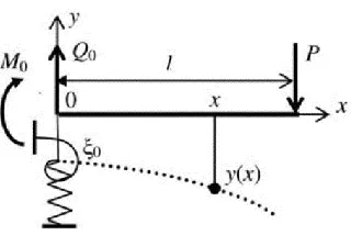
Let us consider the features of inverse problems with numerical differentiation and reduction of measurements using the example of a force element of a mechanical structure. The cantilever beam has a length l and a constant stiffness of the cross section when bending EI, where E is the modulus of elasticity, I is the moment of inertia of the cross section. As can be seen from Fig. 2, one end of the cantilever beam is built into the support, the other end of the beam is free. The beam is subjected to the action of a concentrated load P at the free end. Here the deflections of the beam are measured, the target characteristic is determined, which is the bending moment M0

Fig. 2. Cantilever under a concentrated load

Distinguish the following system elements: the measured object – the beam, the environment (the external load on the beam, the coordinate of the external force, the initial parameters of the elastic line – the transverse displacement and the angle of rotation of the elastic line on the support), MC, ICS. The object under study is the bending moment at the fixed end of the cantilever beam. In the observable system, indirect manifestations of the object under study are measured-the deflections of the beam. By interpreting these measurements, we obtain the most accurate value of the required bending moment.

The deflection function y(x) is given by the results of the joint measurements – by the finite values (counts) y*_(x

i) of the deflections at the longitudinal registration section [xa, xb] of the beam

at the points xi. Taking into account the measurement uncertainty the values of y*(xi), the

approximation polynomial repeats this uncertainty. There are options for choosing a polynomial that runs close to these points. Selection of a metric is generally determined by the nature of the experiment. The least-squares method is effective in the approximation when processing experimental results, it smooths out some inaccuracies in the function y*_{(x) and takes into account}

the uncertainty of the measurements at the node points. The effectiveness of the least-squares method decreases with a decrease in the array of experimental results. In the present paper, for a small number of measured deflections of a beam, we impose a more stringent condition on the approximation problem – the condition of a uniform continuous norm for absolute measurement uncertainty.

The minimum number of measured deflections depends on the characteristics of the cantilever beam, in particular, on the accuracy of setting its length l and the initial parameters – the transverse displacement 0 and the angle of rotation 1 of the elastic line on the support. The

bending moment is determined by three measured deflections under conditions of low accuracy of one of the initial parameters of the elastic line and the coordinate of the point of application of the external force.

When restoring the directly non-measurable target characteristic M0 of the cantilever beam,

we consider the class of inverse problems represented by the function (1), where y(x) is the solution of the initial problem with the differential equation

( )

( )

y x = f x (3)

and fd(x) = P/EI is the forcing function.

According to Loktionov (2017b), to take into account the Saint-Venant's principle, the sensors are placed in the measuring section [xa, xb] outside the beam support zone and outside the

zone of external load on the beam on the approximation grid

The theory of the bending of Euler-Bernoulli beams is the basic theory in the analysis of beams. This theory provides an understanding of the structural behavior of the beam, including under difficult conditions, for example, if the support is elastic (Shi et al. 2014, Wanget al. 2016, Kim 2017).

The initial problem (4) for the Euler-Bernoulli beam has particular solutions

( )

0 1 2 2 3 6

i i i i

y x =  + x +  x +  x (5)

for initial conditions

0 0, 0 1, 0 2

y =  y=  y=  (6)

where 0, 1, 2 are the initial parameters of the elastic line of the beam y(x),  =2 M0 EI= − l 3 ,  =₃ Q₀ EI and Q0 = P. In formula (5), deflections from local deformation on the support are

taken into account.

The model of the beam Timoshenko takes into account the effect of shear deformation on deflections, the cross sections remain flat, but not perpendicular to the deformed axis of the beam. The function y(x) are then

( )

0 1 3 2 2 3 6

y x =  +  − x k xEI GF+  x +  x (7) where k is the shear coefficient, G is the shear modulus of the material, F is the cross section area of the beam.

The results obtained for the parameters 0, 2 and 3 by the method of this paper are also

suitable for the Tymoshenko's beam model, since in (7) the terms with 1 and k with respect to

the variable x are homogeneous.

Together with the directly non-measurable target characteristic of the object M0, the set of

other arguments characterizing the influencing quantities, including those related to the external medium (transverse displacement and the angle of rotation of the elastic line on the support), is transformed into deflections y*_(x

i). By reduction of measurements, we obtain the function f*(x),

which is an approximation to the function f(x) with a minimum value of the level of uncertainty. The set of values {yi*} forms an observation space. This is a finite-dimensional coordinate

Euclidean space of measured deflections on the approximation grid (4). If the accuracy of the transverse displacement and the angle of rotation of the elastic line on the support is small, then the bending moment M0 at the fixed end of the beam can be calculated through the deflections in

the measuring section [xa, xb] in (4). According to Loktionov (2013, 2017b) we use the

one-dimensional Lagrange approximation of the first degree in numerical differentiation. Then the function y"(0) in Eq. (1) are given by the equation

( )

2 1

n

i i

i L y x  =

 



where Li is the Lagrange coefficients, n is the number of approximation parameters (the number

of sensors in the measurement aggregation). The right-hand side of Eq. (8) is the operator A–1 in the formula (2). The accuracy of determining the bending moment M0 through the initial

parameter 2 is determined taking into account the accuracy of the parameters E and I.

Evaluation of measurement reduction efficiency. The efficiency of measurement reduction is related to the optimization of sensor aggregation. Consider two classes of transformation of deflections and, accordingly, two classes of sensors.

Sensors can have the same characteristics. This case corresponds to the class of p -transformation of deflections and sensors. P-transformation is a linear transformation with a uniform continuous norm of absolute measurement uncertainty. The resulted uncertainty of measurements of p deflections, sensor signals and communication channel at all points xi (i = 1,

2, … n) is the same. The limits of the measurements of the sensors yp are the same and equal to

the upper limit supy*_(x

i) on the compact set of real numbers { y*(x1), …, y*(xn)}. Thus

( )

(

( )

)

(

( )

)

( ) ( )

i m i p p i i i

y x y x y y x y x y x

 =  =    = − (9)

where m(y(xi)) is the upper limits of the absolute values of the uncertainty in the deflection

measurements.

We also consider the class of pi-transformation of deflections and sensors with different measurement limits ypi = y(xi). In the pi-transformation we use the following relations

( )

(

)

(

( )

)

m y xi pypi y xi

 =    (10)

In accordance with Cheney and Kincaid (2013), in order to assess the accuracy of measurements and calculations, we introduce the absolute and relative number of conditionality of a problem by relations

( )

(

( )

)

m v m y xi

    (11)

( )

m v p

    (12)

where m(ξ2), m(ξ2) and m(y(xi)) are respectively the upper bounds of the absolute and relative

values of measurement uncertainty ξ2 and the upper limit of absolute values of measurement

uncertainty of deflections y(xi),  and v are respectively the absolute and relative number of

conditionality of the task.

Optimal relations in the aggregation of measuring sensors include the class of transformation, the number and distribution of sensors on the beam. Optimal relationships are obtained by regularizing the aggregation of the sensors and determining the minimal conditionality number for the reduction problem, which is equal to the value of the structural uncertainty of the solution of the problem. The objective function of the reduction problem with the efficiency estimate according to Eq. (11) has the following form

( )

( )

minv=min _m _m y (13)

and according to Eq. (12) has the form

( )

minv_ =min _m _p (14)

The regularization consists in choosing the transformation class of the sensors and the signal of the communication channel and the type of distribution of the nodes of the approximation grid. For all continuous functions on the measuring section [xa, xb] there is no unified strategy for

choosing the optimal grid nodes for the convergence of the measure of the structural error of the measurement reduction problem. Some results have been described (Loktionov 2013, 2017b). In particular, for the p-transformation of deflections y*_(x

(8) reduces to the definition of a compact set of grid nodes in the objective function (in the Lebesgue constant of the second kind):

2 min 0

n

n i= Li

 =



We consider the problem of optimizing the function (15) with the conditions (4) for a known value of the beam length and small accuracy of the values of the transverse displacement 0 and

the rotation angle 1 of the elastic line on the support.

3. The problem with the low accuracy of the beam length and of the angle of rotation of the elastic line at the stationary end of the beam

We transform equation (8) taking into account the known value of the transverse displacement 0

of the elastic line on the support:

( )

2 ₁ 0

n

i i

j L y x 

=  

 



In Section 2 we have analyzed the fundamental relations for the considered problems. Here, computational details are given, following Loktionov (2017b).

If the accuracy of the beam length l and the initial parameter ξ1 is low, then the system of

three equations (5) under condition  =₂ M₀ EI= − l ₃ is solvable with respect to the initial parameter ξ2. Therefore, the three deflections y(xi) are sufficient for determining the initial

parameter ξ2 by formula (16). The approximate polynomial by formula (16) for n = 3 realizes the

formula of the second derivative of the deflection function at a point with coordinate x = 0 by numerical differentiation in ICS. This polynomial should not be a function of both the length l and the initial parameter of the elastic line of the beam 1. In accordance with the method of

undetermined coefficients, the following conditions must be satisfied. We use the method of undetermined coefficients. The following conditions must be met:

3 1 3 ₂ 1 3 3 1 0 2 0 i i i i i i i i i L x L x L x = = =  ₌   ₌    = 







The conditions of formulas (17) are satisfied with the Lagrange coefficients

(

)

(

)(

)

(

)

(

)(

)

(

)

(

)(

)

1 2 3 1 2 1 3 1

2 1 3 2 2 1 3 2

3 1 2 3 3 1 3 2

2

2

2

L x x x x x x x

L x x x x x x x

L x x x x x x x

 = − + _ − − _  _{= +  − − }  _{ }    = − + − −     (18)

An approximate solution according to Eq. (16) takes into account deflections y*_(x

i), including

errors of the initial data within the uncertainty of each deflection value. The total absolute uncertainty of the value of ξ2, according to Eq. (16) with a set of three deflections, will have the

form

( )

2 _i=1L y xi i

The relative uncertainty of ξ2 can be written as

( )

2 _i=1L y xi i 2

 =



3.1 Uneven distribution of nodes

Here we will present the details of the above method of regularizing sensor aggregation and determining the minimal conditionality number for the reduction problem.

P-transformation of deflections y(xi). Taking into account the formulas yp=y(x3), (9), (11),

(13), (16), and (19), the absolute conditionality number for the reduction problem is

3 1 i i

v_ =



The problem is regularized with the absolute conditionality number (21). We substitute the coefficients (18) into Eq. (21), we obtain

(

) (

)

(

)

(

)(

)

3

2 3 1 1 3 2 3 2 1 2 3 2 1 3 2

1 i 2

i= L = x +x x x +x +x x −x   x x x x −x x −x 



The function (22) on the measuring section [xa, xb] has a boundary minimum at the point x3

= xb. To obtain the optimal values of the coordinates of the points x1 and x2, we use the equations

(

)

(

)





Taking into account the solution of the system of equations (23), the result of the regularization of the problem for the absolute conditionality number has the distribution of the coordinates of the deflections

(

)

(

)

(

)

( )

1 3

2 3

3 _{3 max}

1 3 3 2 3 2 2 3

1 3

b

x x

x x

x x x

 _{= −} _{− + + −} _  _{ }  _{= − +}   = =   (24)

On the measuring section [xa, xb], for accuracy with three significant digits, we obtain the

distribution of coordinates of the interpolation nodes

1 3

2 3

3

0.196 0.186 0.732 0.695

0.950

b

x x l

x x l

x x l

= =   = =   _{= =}  (25)

and the minimal absolute conditionality number is 80.2/l2_.

In determining the relative conditionality numbers on the measuring section [xa, xb], we

introduce relations

( )

0 1xi y xi

 +   (26)

( )

(

)

  _ − _ (27)

The accuracy of determining the relative conditionality numbers is determined by the accuracy of Eq. (27). Taking into account Eq. (27) at xi= x3, Eqs. (3), (12), (14) and (20) we find

the following expression for the relative conditionality number for the reduction problem

(

)

2

3 1 3 3 _{i 1} i 2

v_ =x −x l



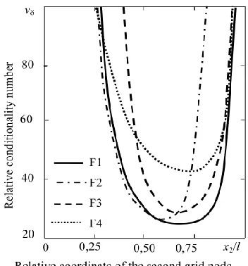
By means of regularization, taking into account (28) and the coefficients (18), we obtain the coordinate distribution of the grid nodes according to Eqs. (25), the minimal relative conditionality number of the problem is 24.7.

As seen in fig. 3, the deviation of coordinates from the optimal values increases the uncertainty of the result of solving the problem. The relative conditionality number (28) in Fig. 3 is represented by the lines F1 – F4. The line F1 is characterized by the optimal values of the coordinates x1 and x3 in (25). Lines F2– F4 are characterized by non-optimal values of x1 or x3

coordinates. The F2 line is characterized by non-optimal x1/l = 0.0500 < 0.186 and optimal x3.

The F3 line is characterized by non-optimal x1/l = 0.300 > 0.186 and optimal x3. The F4 line is

characterized by non-optimal x3/l = 0.800 < 0.950 and optimal x1. In the absence of optimization,

the relative conditionality number of the problem is more than 24.7. For example, if x2 0.3l or

x2 > 0.9l, the relative conditionality number increases more than 2.5 times and becomes more than

65.

Fig. 3. The conditionality number according to Eq. (28) with Lagrange coefficients according to the formulas (18)

Pi-transformation of deflections. Substituting expressions (10), (13), (16), (19) and ypi =

y(xi) into Eq. (11) we arrive at the equation

( )

( )

2 1

m p i= L y xi i

  = 



( )

( )

(

)

(

)

2 3 ₁ 1 3 3 1 3 3

m  py x _i= L xi i xi l  x x l 

  = _



By using Eq. (11), we find the absolute conditionality number of the problem ξ2

(

)

(

)

3 2 2

3 3

1 i i 1 i 3 1 3

i

v_=



The result of the regularization of the problem by a numerical method is the distribution of the coordinates of the grid nodes with three significant digits

1 3

2 3

3

0.0526 0.0500 0.244 0.232

0.950

a

b

x x x l

x x l

x x l

= = =



 _{= =}



 = = 

(32)

the minimal absolute conditionality number for the reductionality problem is 6.00/l2_.

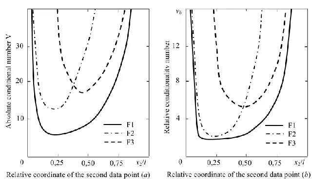
As can be seen from fig. 4 a, the deviation of coordinates from the optimal values increases the uncertainty of the result of solving the problem, in particular, when the x2 coordinate changes

in accordance with the F1 line, and also with a decrease in the x3 coordinate in accordance with

the F2 line or with an increase in the x1 coordinate in accordance with F3 line. As shown in Fig.

4 a, the line F1 corresponds to the coordinates of the grid nodes x1/l = 0.0500 and x3/l = 0.950,

the line F2 corresponds to the coordinates x1/l = 0.0500 and x3/l = 0.700, the line F3 corresponds

to the coordinates x1/l = 0.200 and x3/l = 0.950. Hereinafter,, V = l2. In the absence of

optimization, the absolute conditionality number is more than 6.00/l2_{. In particular, if x}

2 > 0.75l,

or if x2 > 0.45l and x3 0.70l, the absolute conditionality number of the problem increases more

than 4 times and becomes more than 24/l2_.

Considering Eqs. (10), (12), (20) and (27) we obtain the relative conditionality number of the problem

(

)

3 2

1 i i 1 i 3 2

i

v_ =



Fig. 4. The conditionality numbers of problem (16), pi-transformation of deflections. (a) Absolute conditionality number to Eq. (31); (b) Relative conditionality number to Eq. (33)

As can be seen from Fig. 4 b, if the conditions (32) are not satisfied, then the relative conditionality number of the problem exceeds the optimal value. In particular, if x2 > 0.80l or x2

> 0.55l and x3 0.70l, then the relative conditionality number increases more than 4 times and

becomes more than 9. The connection of the lines F1, F2 and F3 with the coordinates of the grid nodes in Fig. 4 b coincides with Fig. 4 a.

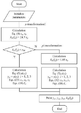
The selection and placement of sensors in subsection 3.1 is shown in Fig. 5.

It is necessary to enter the predetermined error of the measuring device with sensors and the communication channel p, the approximate values of the beam length l and the initial parameter

1, as well as the value of M equal to the desired maximal relative error of the initial parameter

2.

3.2 Uniform distribution of nodes

Expectedly worse results are obtained with the regularization of only the length and placement of the measuring section [x1, x3] with a uniform distribution of the sensors along the beam under

condition

(

)

2 1 3 2

x = x +x (34)

Eqs (17) are satisfied by the Lagrange coefficients

(

)

(

)

(

)

(

)

(

)

2

1 1 3 1 3 1

2

2 3 1

2

3 1 3 3 3 1

2 3

16

2 3

L x x x x x

L x x

L x x x x x

 _{= − +}  ₋ 

  



= −



 _{ }

= − + −

 _{ }



(35)

(

)

(

)

3 2 2

1 3 1 3 1 3 3 1

1 i 2 4 3

i

v_=



To minimize the function (36), the value of the coordinate x3 must be equal to xb. Using the

first of Eqs. (23) we obtain an algebraic equation of the fourth degree with unknown x1

4 3 2 2 3 4

1 20 3 1 3 14 3 1 3 4 3 1 3 0

x + x x − x x − x x +x = (37)

The result of solving Eq. (37) by the Descartes-Euler method with an accuracy of three significant digits is the distribution of coordinates of the grid nodes

1 3

2 3

3

0.214 0.203 0.607 0.576

0.950

b

x x l

x x l

x x l

= =



 = =



 = = 

(38)

and the minimal absolute conditionality number of uncertainty of the problem is 88.5/l2_.

The result of the regularization using formulas (28) and (35) is the distribution of coordinates of grid nodes according to formulas (38) and the minimal relative conditionality number of problem 27.3.

In the pi-transformation of deflections by regularization using the numerical method and formulas (31), (33), (35), we find the coordinate distribution of the grid nodes

1 3 2 3 3 0.0526 0.0500 0.526 0.500 0.950 b

x x l

x x l

x x l

= =   = =   = =  (39)

the minimal absolute conditionality number of problem 8.90/l2 _{and the minimal relative}

conditionality number of problem 2.74. The values of the minimal conditionality numbers for the pi-transformation of deflections, when the nodes are distributed uniformly, and only the position of the measuring section [xa, xb] is optimized, is one and a half times greater than when the nodes

have a variable step and are optimal.

4. The length of the beam and the displacement of the support across the beam are known with low accuracy

Let's change the formula (8) taking into account the known value of the slope angle of the elastic line at the fixed end of the beam

( )

2 ₁ 1

n

i i i

i L y x x



=  

 



Three deflections y(xi) are sufficient to determine the initial parameter ξ2 according to

formulas (5) and (40) if the length of the beam and the displacement of the support across the beam are known with low accuracy. Formula (40), when n = 3, is realized in numerical differentiation with the help of a measuring and computing system. For this, conditions (17) must be satisfied in accordance with the method of undetermined coefficients. These conditions are satisfied by Lagrange coefficients

(

)

(

)

(

)

3 3

1 3 2

3 3

2 3 1

3 3

3 2 1

2

2

2

L x x K

L x x K

L x x K

 = − −   _{= −}    = − −  (41) where

(

)(

)(

)(

)

K= x −x x −x x −x x x +x x +x x (42)

According to the method described in Sections 2 and 3, the following results are obtained.

4.1 Three unevenly located nodes

P-transformation of deflections. The problem is regularized with an absolute conditionality number according to formula (21). Substituting the coefficients (41) into (21), we obtain

(

)

(

)(

)(

)

3 2 2

1 1 3 3 2 1 3 2 1 2 1 3 2 3

1Li 4 x x x x x x x x x x x x x x

= = + +  − − + + 

The function according to formula (43) on the measuring section [xa, xb] assumes a minimum

value when x1 = xa and x3 = xb. Using the second of Eqs. (23), we obtain the coordinate of the

second node

(

) (

)

2 2 3 1 3 3 1

x = x −x _ x −x _ (44)

Consequently, in (4), to within three significant digits, we obtain the distribution of coordinates of the grid nodes

1 3

2 3

3

0.0526 0.0500 0.668 0.635

0.950

a

b

x x x l

x x l

x x l

= = =



 = =



 = = 

(45)

the minimal absolute conditionality number 30.3/l2_.

As can be seen from Fig. 6 a, if the grid coordinates distribution does not coincide with the distribution (45), the absolute conditionality number of the problem is greater than the optimal value. In particular, if x2 > 0.85l or if x2 > 0.77l and x3 0.85l, or if x2 0.40l and x1 > 0.20l, then

the absolute conditionality number of the problem increases more than 2 times and becomes more than 60/l2_.

The result of the regularization of formula (28) with allowance for the coefficients (41) is the distribution of coordinates of grid nodes according to formulas (45), the minimal relative conditionality number of of problem 9.34. As can be seen from Fig. 6 b, if the distribution of the grid coordinates does not coincide with the distribution (45), the relative conditionality number of the problem, like the absolute conditionality number, is greater than the optimal value. In particular, if x2 > 0.88l or if x2 > 0.80l and x3 0.85l, or if x2 0.40l and x1 > 0.20l, then the

relative conditionality number increases more than 3 times and becomes more than 30.

Pi-transformation of deflections. We regularize the problem with the absolute conditionality number by the formula (31). We substitute the coefficients (41) into the formula (31), we obtain the coordinate distribution of the deflections with the accuracy of three significant digits

1 3

2 3

3

0.0526 0.0500 0.183 0.174

0.950

a

b

x x x l

x x l

x x l

= = =



 = =



 = = 

(46)

and minimal absolute conditionality number of the problem is 3.89/l2_.

As shown in Fig. 7 a, the line F1 corresponds to the coordinates of the grid nodes x1/l =

0.0500 and x3/l = 0.950, the line F2 corresponds to the coordinates x1/l = 0.0500 and x3/l = 0.850,

the line F3 corresponds to the coordinates x1/l = 0.100 and x3/l = 0.950. In the absence of

optimization, the absolute conditionality number is more than 3.89/l2_{. In particular, if x}

2 > 0.80l,

or if x2 > 0.63l and x3 0.85l, the absolute conditionality number of the problem increases more

Fig. 6. The conditionality numbers of problem (40), p-transformation of deflections. (a) Absolute conditionality number to Eq. (21); (b) Relative conditionality number to Eq. (28)

Fig. 7. The conditionality numbers of the problem (40), pi-transformation of deflections. (a) Absolute number to Eq.(31); (b) Relative number to Eq. (33)

The result of regularization by the formula (33) with the coefficients (41) is the coordinate distribution of the deflections according to the formulas (46) and the minimal relative conditionality number of problem 1.20. As shown in Fig. 7 b, the line F1 corresponds to the coordinates of the grid nodes x1/l = 0.0500 and x3/l = 0.950, the line F2 corresponds to the

coordinates x1/l = 0.100 and x3/l = 0.950, the line F3 corresponds to the coordinates x1/l = 0.050

and x3/l = 0.850. In the absence of optimization, the relative conditionality number is more than

1.20. In particular, if x2 > 0.72l or x2 > 0.65l and x3 0.85l, then the relative conditionality number

4.2 Three nodes with a constant pitch

The predictably worst results were obtained in case of regularization only of the length and measuring section [xa, xb] with regular distribution of deflection sensors on the beam, when

Lagrange coefficients (41) satisfy Eqs. (17) providing (34).

At p-transformation of deflections the following distribution of data coordinates is obtained

1 3 2 3 3 0.0709 0.0674 0.535 0.509 0.950 b

x x l

x x l

x x l

= =   = =   _{= =}  (47)

the minimal absolute conditionality number is 34.3/l2 _{and minimal relative conditionality number}

is 10.6.

For the pi-transformation of deflections, formulas (39) for the optimal distribution of deflection coordinates are obtained, the minimum absolute conditionality number of problem 7.32/l2 _{and the minimum relative conditionality number 2.26. The values of the minimum}

conditionality numbers for the pi-transformation of deflections, when the nodes are distributed evenly, are 1.9 times larger than when the nodes are distributed unevenly and optimally.

5. Experimental researches of variants of transformation of deflections

The developed mathematical models of measurements reduction research have been experimentally tested. The tests were carried out on a cantilever beam with the following parameters: modulus of elasticity E = 200 GPa, type of section: rectangle (height h = 40.0 mm, width b = 10.0 mm), moment of inertia I = bh3_{/12 = 5.33 mm}4_{, length l = 1.00 m.}

The values of the initial parameters of the elastic line of the beam: 0 = − 8.010-3 mm, 1 =

1.010-5_{. Concentrated load P = 69.0 N. The deflection calculated with the formula (5) at x} 3 =

0.950 l is 1.85 mm. In particular, in experiments on subsection 4.1, sensors with an accuracy class of 0.5 (a reduced error of 0.5%) were used. The reduced error is determined by formula

error Reduced error

Maximal value of the measur Absolute

ing inte 100

rval

= (48)

The results of the obtained error of measurements of deflections and bending moment at a fixed end of the beam are given in Tables 1 and 2 to verify the accuracy of the developed method of reduction of measurements.

Coordinates of deflections

xi

Values xi, m

Limits of measurement of sensors, m

Calculated Measured

y(xi), m m(y(xi)),

m yi, m

y(xi),

m

x1 5.0010 -2

20010-5 − _1.49₁₀ -5

110-5 − ₂₁₀-5 −

0.510-5

x2 0.635 20010-5 −

0.96010-3

110-5 − ₉₅₁₀-5 ₁₁₀-5

x3 0.950 20010-5 − 1.8510

-3

110-5 − ₁₈₆₁₀ -5

− 110-5

M, % 4.7 1.9

For p-transformation of deflections, minimal relative conditionality number of the problem is 9.34. For maximum pre-determined deflection, sensors with the upper range limit of 2 mm and absolute uncertainty of measurements of 0.01 mm were chosen. The expected calculated reduced uncertainty of measuring the bending moment on the support is 0.5%9.34 = 4.7%. The experimentally obtained value is 1.9%.

Coordinates of deflections

xi

Values xi, m

Limits of measurement of sensors, m

Calculated Measured

y(xi), m m(y(xi)),

m yi, m y(xi), m

x1 5.0010 -2

20010-7 −

14910-7

110-7 −

15010-7

− 110-7

x2 0.174 10010-6 −

92010-7

510-7 − ₉₂₁₀-6 _{less than}

110-7

x3 0.950 20010-5 −

18510-5

110-5 −

18610-5

− 110-5

M, % 0.6 0.5

Table 2. Errors of deflections and bending moment for pi-transformation of deflections

For pi-transformation of deflections, minimal relative conditionality number of the problem is 1.20. For optimal coordinates of the three sensors, in accordance with Eqs. (35), deflections were calculated and sensors with different ranges (2 mm or less) were selected. The expected calculated reduced uncertainty of measuring the bending moment on the support is 0.5%1.20 = 0.6%. The experimentally obtained value is 0.5%. The experimental accuracy of measuring the bending moment for pi-transformation of deflections is four times higher than the accuracy for the p-transformation.

6. Conclusions

It was proved that there is the possibility of a significant (several times) increase in the accuracy of determining the directly unmeasured characteristic of the mechanical structure on the basis of the theory of inverse problems, the method of reduction of measurements.

Improving the polynomial approximation of Lagrange and numerical differentiation in the IVS resulted in an optimal arrangement of sensors on the element of the mechanical structure.

The proposed method takes into account the uncertainty of the value of the initial parameter of the elastic line of the beam, which includes the transverse displacement or the angle of rotation on the support, as well as the low accuracy of the coordinate of the concentrated load.

The proposed technique, depending on the required accuracy and the level of the experimental base, makes it possible to decide on the type of approximation: apply a uniform arrangement of the sensors along the beam or apply regularization to improve accuracy.

The proposed technique, with the use of regularization, allows one to choose between rather simple measurement aggregations of sensors with p-transformation of deflections and more complex aggregations with pi-transformation of deflections to reduce the error.

References

Al-Azzawi AA, Theeban DM (2010). Large Deflection of Deep Beams on Elastic Foundations, Journal of the Serbian Society for Computational Mechanics, 1, 88-101.

Bogusz J, Figurski M, Nykiel G, Szolucha M (2012). GNSS-based multi-sensor system for structural monitoring applications, Journal of Applied Geodesy, 6(1), 55-64.

Chekushkin VV, Mikheev KV, Panteleev IV (2015). Improving Polynomial Methods of Reconstruction of Functional Dependences in Information-Measuring Systems, Meas. Tech., 58(4), 385-392.

Cheney EW, Kincaid DR (2013). Numerical Mathematics and Computing. Thomson Brooks/Cole, Belmont, California, USA.

Dung CV, Sasaki E (2016). Numerical Simulation of Output Response of PVDF Sensor Attached on a Cantilever Beam Subjected to Impact Loading, Sensors, 16(5), 601.

Gere JM, Timoshenko SP (1997). Mechanics of Materials. PWS Pub. Co.Boston, Massachusetts, USA.

Haque ME, Zain MFM, Hannan MA, Rahman MH (2015). Building structural health monitoring using dense and sparse topology wireless sensor network, Smart Struct. Syst., 16(4), 607-621. Huang HB, Yi TH, Li HN (2016). Canonical correlation analysis based fault diagnosis method

for structural monitoring Sensor networks, Smart Struct. Syst., 17(6), 1031-1053.

Kara IF (2016). Flexural performance of FRP-reinforced concrete encased steel composite beams, Struct. Eng. Mech., 59(4), 775-793.

Kaveh A, Zolghadr A (2016). Optimal analysis and design of large-scale domes with frequency constraints, Smart Struct. Syst., 18(4), 733-754.

Kim YW (2015). Analytic solution of Timoshenko beam excited by real seismic support motions, Struct. Eng. Mech., 62(2), 247-258.

Korytov MS, Shcherbakov VS, Shershneva EO, Breus IV (2016).Approximation methods for the actual trajectory of load carried by overhead crane to the required one – a comparative analysis, Journal of the Serbian Society for Computational Mechanics, 2, 45-56.

Loktionov AP (2007. A principle of constructing the system for measuring the FV takeoff weight and center-of-mass position on the basis of measurement reduction, Russian Aeronautics, 50(2), 178 – 185.

Loktionov AP (2009). Strukturnaja reguljarizacija podsistemy preobrazovatel'nogo komponenta preobrazovatel'no-vychislitel'nyh system. Kursk. gos. tehn. un-t, Kursk, Russia.

Loktionov AP (2013). Regularization of the lattice time function of the signal in the communication channel, Telecommunications and Radio Eng., 72(2), 161-171.

Loktionov AP (2017a). Improving the Polynomial Approximation of an Object Characteristic

that is not Directly Measurable by Using Measurement Reduction

https://link.springer.com/article/10.1007/s11018-017-1089-3, Meas. Tech., 59(10), 1042-1050.

Loktionov AP (2017b). A measuring system for determination of a cantilever beam support moment, Smart Struct. Syst., 19(4), 431-439.

Lü C, Liu W, Zhang Y, Zhao H (2012). Experimental Estimating Deflection of a Simple Beam Bridge Model Using Grating Eddy Current Sensors, Sensors, 12(8), 9987-10000.

Ozbey B, Erturk VB, Demir HV, Altintas A, Kurc OA (2016). A Wireless Passive Sensing System for Displacement/Strain Measurement in Reinforced Concrete Members, Sensors, 4, 1-17.

Sayyad AS, Ghugal YM, Shinde PN (2015). Stress analysis of laminated composite and soft core sandwich beams using a simple higher order shear deformation theory, Journal of the Serbian Society for Computational Mechanics, 9(1), 15-35.

Wang T, He T, Li H (2016). Effects of deformation of elastic constraints on free vibration characteristics of cantilever Bernoulli-Euler beams, Struct. Eng. Mech., 59(6), 1139-1153. Yang Y, Huang H, Sun L (2017). Numerical studies on the effect of measurement noises on the

online parametric identification of a cable-stayed bridge, Smart Struct. Syst., 19(3), 259-268. Yi TH, Zhou GD, Li HN, Zhang XD (2015)/ Optimal sensor placement for health monitoring of high-rise structure based on collaborative-climb monkey algorithm, Struct. Eng. Mech., 54(2), 305-317.

Zelenkova MV, Skripka VL (2015). Prospects for Improving Calibration Techniques using a Measurement Reduction Apparatus, Meas. Tech., 58(5), 491-495.