(10.24874/jsscm.2019.13.02.02)
MODELING OF DAMAGED CONCRETE USING INITIAL
DEGRADATION PARAMETER
Dragan Rakić1*, Vladimir Dunić1, Miroslav Živković1, Nenad Grujović1, Dejan Divac2
1 University of Kragujevac, Faculty of Engineering, 6 Sestre Janjić Street, 34000 Kragujevac
e-mail: [email protected]
2 Jaroslav Cerni Water Institute, 80 Jaroslava Černog Street, 11226 Belgrade
*corresponding author
Abstract
A stress-strain history in the material of real concrete structures is usually unknown. An effect of concrete degradation is analyzed to describe how the initial degradation parameter can describe the stress-strain history. The idea is to introduce the initial damage of the structure by the degradation parameter to calculate the internal variables of the constitutive model. Six numerical examples are proposed to verify the methodology for various loading conditions. Based on the obtained results, it was shown that unknown stress-strain history could be successfully represented using the original material parameters and the initial degradation of the concrete. The stress-strain behavior of the damaged concrete is successfully simulated and essential for the structural analysis of civil engineering structures.
Keywords: concrete model, damage, numerical method, FEM, stress-strain history
1. Introduction
The suggested methodology is verified by several numerical examples: monotonic and cyclic uniaxial and biaxial tension and compression loading (Lee 1996; Lubliner et al. 1989; Omidi & Lotfi 2010). The stress-strain history is considered via degradation parameter. The initial material parameters are used and the initial degradation is computed in independent test. The results of the complete stress-strain history tests and the tests with the initial material degradation are compared.
It is shown that it is possible to take into account the stress-strain history by initial degradation parameter and the initial material parameters of concrete. This is very important for the simulation of the real concrete structures, because the stress-strain history is unknown.
2. Fundamental relations
2.1 Damage concrete constitutive model
Based on the theory of plasticity (Kojic & Bathe 2004), it is possible to decompose the strain tensor into the elastic and plastic part as:
e p
e e e . (1)
In that case, the constitutive relation can be expressed in the following form:
: e : p
σ C e C e e . (2)
The stiffness matrix C is related to the stiffness degradation variable d (Lee 1996; Lee & Fenves 1998):
1 d
0
C C , (3)
where C0 is the initial elastic stiffness tensor. This gives the possibility to decompose the stress
tensor to the effective part σ and to the stiffness degradation
1d
:
1 d
σ σ, (4)
where the effective part can be obtained using the initial elastic stiffness tensor:
0: p
σ D e e (5)
The plastic potential function is given as:
pI1 σ S (6)
where S S S: is the deviatoric stress norm, S σ
mI is the deviatoric effective stress,1 tr
I σ is the first stress invariant, and p is the dilatancy parameter. The plastic flow rule is given as (Lee, 1996):
p
ε
where is non-negative plastic consistency parameter. For the multidimensional problems, the relation between the damage variables κ and the plastic strain tensor can be defined by eigen
values of plastic strain denoted by
^
( ) as (Lee 1996; Lee & Fenves 2001; Lee & Fenves 1998):
,ˆ :ˆp
κ h κ σ e (8)
where the matrix
h
defines the influence of tension and compression loading. The further derivation gives:
,ˆ : κ H κ σ , (9)
where:
,ˆ ,ˆ : ˆ H κ σ h κ σσ . (10)
For the concrete, the yield function is given as [1]:
c
0F σ c κ (11)
where F σ
is the scalar function of stress invariants, and c κc
is the cohesion. Modified yieldfunction (Lee 1996) has the following form:
1 max
1 3
( , ) 0
1 2 c
F I c
σ κ S κ κ (12)
where: cc
κ
c
κ is the cohesions which is equal to the effective compressive stress, 1tr 3
m
σ is the mean effective stress, and
max is the eigen stress maximum value of σ. In theyield function, there are following parameters and
related to the biaxial loading conditions (Lee & Fenves, 1998).The basic assumption is that the damage variables κ
t, c
T are related to the stress and thestiffness degradation (Lee 1996; Lubliner et al. 1989):
/ 0
/ / / / / /
/
1
t c
t c t c t c t c t c t c
t c
f
f a
a
(13)
where ft c/ 0 is initial yield stress, and the function t c/ is:
/ 1 / 2 / /
t c at c at c t c
(14)where the parameter
а
t c/ is related to the shape of function.The relations between the degradation and damage variables is given as:
// / / / / 1 1 1 t c t c c bt c t c t c
t c
d a
a
The input parameters which define the shape of stress–damage relationship curve are the compressive degradation Dc for the maximal compressive stress fcm, and the tensile degradation
t
D for the half of the yield tension stress ft0. For the known degradation parameters Dt c/ and the parameter аt c/ , it is possible to find bt c/ ct c/ .
For the multidimensional problems, the degradation is obtained by interpolation between the values for compression and tension:
1 1 c 1 t
d d κ d κ (16)
For the cyclic loading, it is necessary to introduce the parameter of stiffness recovery
ˆ 0
1 0
ˆs σ s s r σ as:
ˆ
1 1 c 1 t
d d κ s σ d κ (17)
wheres0 is the minimal value of s.
2.2 Initial damage formulation
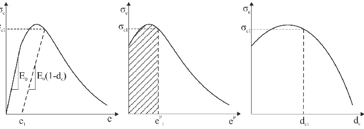
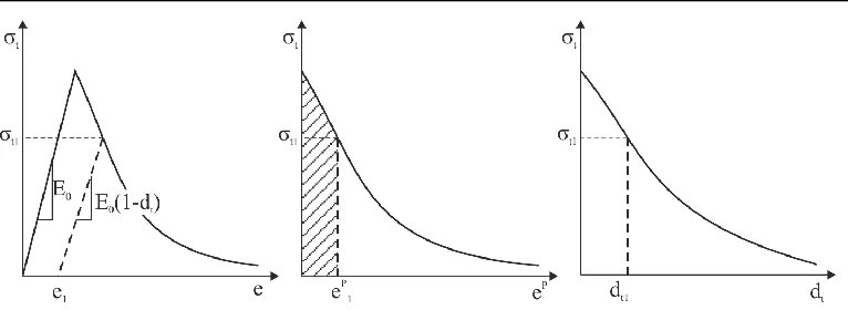
It is of great interest to define methodology for the identification of material parameters necessary for numerical simulations of such structures. In this paper, the authors formulated the relationship between the stress-strain history and the degradation variable, based on theory of damage plasticity concrete constitutive model. The degradation variable is used because it can be identified by simple non-destructive experimental tests. As it can be noticed in eq. (13), the degradation variable is related to the strength of the material. So, it is necessary to know current degradation state to calculate the stress and strain. The general relation between stress vs. strain, plastic strain and degradation is given in Fig. 1 for compression and in Fig. 2 for tension.
Fig. 2. Plasticity damage model in tension a) total strain vs. stress, b) plastic strain vs. stress, c) degradation vs. stress
In the previous figures, the total strain, plastic strain and degradation from previous stress-strain history are denoted by subscript 1, for tension and compression. It can be noticed that the strength of the material is changed, so the initial parameters are not correct for further simulation of the mechanical behavior. For such case, it is necessary to identify material parameters. So, the proposition is to use the computed value of degradation as input value and the initial material parameters. The hatched surface in Fig. 1 and Fig. 2 correspond to the energy dissipated for plastic strain in stress-strain history.
Based on eq. (13), it is obvious that strength of the material is function of damage variables where
/ 0 t c
f is the yield stress of the material, which can be obtained from maximal strength of the
material ' / t c
f and the material constant at c/ as (Lee, 1996):
2 / '/ / 0
/
1
4
t c
t c t c
t c
a
f f
a
. (18)
For the known value of degradation, the damage variable can be obtained from eq. (14) and eq. (15) as:
//
2
/ 1 / 1 1 /
t c t c
b c
t c at c dt c
, (19)
/
/ / / 1 2 t c t ct c t c
a a
. (20)
It is possible to measure the Young’s modulus by ultrasound technique, and to identify the degradation of the material stiffness from the constitutive relations as:
1
0E d E . (21)
This relation gives the degradation value in following form:
0
1 E
d E
. (22)
3. Methodology verification
Verification of the proposed methodology was carried out through six numerical examples using program PAK (Kojić et al. 1999). The simulation of the uniaxial and biaxial test under monotonic compression and monotonic tension loading was performed, as well as the simulation of uniaxial pressure and uniaxial tensile cyclic loading (Lubliner et al. 1989; Lee & Fenves 1998; Omidi & Lotfi 2010). All tests were performed using a single linear hexagonal finite element of unit dimensions (Kojić et al. 1999; Živković 2006). In all test examples, the same material parameters were used, as it is given in
Table 1. Material parameters
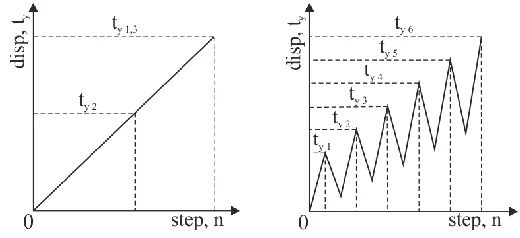
Each of the test examples consisted of three numerical simulations. In the first simulation, the maximum load was applied (ty1,3 in Fig. 3a and ty6 in Fig. 3b). In the second simulation, the load
was set to an arbitrary level, so the plastic strain and the material degradation occurred (ty2 on
Fig. 3a and Fig. 3b). This solution represents a previous stress-strain history.
Fig. 3. Load functions a) monotonic load, b) cyclic load
In the third simulation, the maximum load value was applied, but with the initial degradation equal to the degradation at the end of the second simulation. In this way, the model behavior was analyzed including the stress-strain history via the initial degradation parameter.
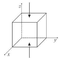
Due to the symmetry of the problem, one-eighth of the model was modeled in all examples, using the symmetry boundary conditions. The numerical examples with a monotonic load were solved in 100 time increments, while the examples with cyclic load were solved in 1100 time increments. The load was applied as displacement of one or two sides of the element.
3.1 Compression loading examples
The compression loading conditions were investigated in three examples. The first example consisted of three numerical simulations of uniaxial monotonic loading test (Fig. 4). The first simulation considered total stress-strain history shown as “full path” in Fig. 5. The previous stress-strain history was obtained by the second simulation which is stopped before the end. The degradation level of the structure was recorded. The beginning of the third simulation is the end of the second one, but with the initial degradation as the input parameter. The dependences of
E [GPa] [-] ' c f [MPa] ' t f [MPa] c G [N/m] t G [N/m]
[-] p
[-] 0 s [-] c D [-] t D [-] ac [-] at [-] γ [-]
axial stress vs. axial strain, plastic strain and degradation were shown in Fig. 5, for the performed simulations.
Fig. 4. Uniaxial compression test
Fig. 5. Uniaxial compression test a) axial total strain vs. axial stress, b) axial plastic strain vs. axial stress, c) degradation vs. axial stress
The same procedure was repeated for the second example which considered uniaxial pressure test under cyclic loading conditions. In this case, six cycles were performed in the first simulation as it is shown in Fig. 3b, to obtain a characteristic of the material behavior. The second simulation was stopped after the second cycle (ty2 on Fig. 3b) and the degradation value was recorded. The
third simulation was carried out to the same level as the first one, but including the initial degradation from the end of the second simulation. The dependences of stress vs. strain, plastic strain and material degradation were shown Fig. 6, for the performed simulations.
Fig. 6. Uniaxial cyclic compression test a) axial total strain vs. axial stress, b) axial plastic strain vs. axial stress, c) degradation vs. axial stress
Fig. 7. Biaxial compression test
Fig. 8. Biaxial compression test a) axial total strain vs. axial stress, b) axial plastic strain vs. axial stress, c) degradation vs. axial stress
3.2 Tension loading examples
The tension loading conditions were also investigated in the same three set of examples. The first example considered monotonic tensile loading conditions (Fig. 9). The proposed three simulations were performed to obtain “full path” of stress-strain history, and the results with included “initial degradation” as the input parameter of the simulation. The results of simulation were shown in Fig. 10.
Fig. 10. Uniaxial tension test a) axial total strain vs. axial stress, b) axial plastic strain vs. axial stress, c) degradation vs. axial stress
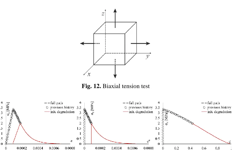
The cyclic and biaxial loading conditions were investigated by prescribed procedure given in previous subsection for compressive loading conditions. The three simulations were performed to verify the functionality of the proposed methodology. The results for the cyclic loading conditions are given in Fig. 11. The monotonic biaxial tensile loading simulation results are given in Fig. 13.
Fig. 11. Uniaxial cyclic tension test a) axial total strain vs. axial stress, b) axial plastic strain vs. axial stress, c) degradation vs. axial stress
Fig. 12. Biaxial tension test
4. Discussion and conclusions
The mechanical behavior of real materials strongly depends on previous stress-strain history. So, the initial material parameters of the structure will not match the material parameters that describe the behavior of the structure after multiple loading-unloading cycles. It is essential to know the previous material stress-strain history. The authors proposed the methodology to describe the stress-strain history of material using a variable that can be measured indirectly by non-destructive methods. The degradation variable is considered as appropriate for the concrete constitutive model based on damage plasticity. The degradation variable can be obtained from the initial and current elasticity modulus and by the proposed procedure to calculate the damage variable.
Verification of the proposed methodology was carried out through six numerical tests. All presented tests contain three numerical simulations showing the stress path for the full stress-strain history, then the arbitrary load solution representing the unknown stress-stress-strain history, as well as the numerical solution of the problem by using initial damage from the end of the previous simulation, as the “unknown” stress-strain history.
Based on the results, one can notice that the introduction of initial degradation gives identical model behavior by applying initial material parameters as well as a model that has undergone some stress-strain history. This conclusion is crucial for practical application in stability analyses of concrete structures such as arch dams that have been in operation for a long period of time, and which undergo a large number of loading cycles (increasing and decreasing accumulation levels).
Acknowledgements: The authors acknowledge support of the Ministry of Education, Science and Technological Development, Republic of Serbia, grants TR32036 and TR37013.
References
Kojic M & Bathe KJ (2004). Inelastic Analysis of Solids and Structures (1st edition). Springer. Kojić M (1996). The governing parameter method for implicit integration of viscoplastic
constitutive relations for isotropic and orthotropic metals. Computational Mechanics, 19, 49-57.
Kojić M, Slavković R, Živković M, & Grujović N (1999). PAK-finite element program for linear and nonlinear structural analysis and heat transfer. Kragujevac: University of Kragujevac, Faculty of Engineering.
Lee J (1996). Theory and implementation of plastic-damage model for concrete structures under cyclic and dynamic loading. Berkeley, California: Department of Civil and Environmental Engineering, University of California.
Lee J & Fenves G (2001). A return mapping algorithm for plastic-damage models: 3-D and plane stress formulation. Int. Journal for Numerical Methods in Engineering, 50, 487-506. Lee J & Fenves GL (1998). A plastic damage concrete model for earthquake analysis of dams.
Earthquake Engineering Structural Dynamics, 27, 937-956.
Lubliner J, Oliver J, Oller S, & Onate E (1989). A plastic-damage model for concrete. Int. Journal of Solids and Structures, 25, 299–326.
Vasanelli E, Sileo M, Calia A, & Aiello MA (2013). Non-destructive Techniques to Assess Mechanical and Physical Properties of Soft Calcarenitic Stones. Procedia Chemistry, 8, 35-44.