www.theoryofcomputing.org
A Chasm Between Identity and Equivalence
Testing with Conditional Queries
Jayadev Acharya
∗Clément L. Canonne
†Gautam Kamath
‡Received December 11, 2015; Revised February 14, 2018; Published December 19, 2018
Abstract: A recent model for property testing of probability distributions (Chakraborty et al., ITCS 2013, Canonne et al., SICOMP 2015) enables tremendous savings in the sample complexity of testing algorithms, by allowing them to condition the sampling on subsets of the domain. In particular, Canonne, Ron, and Servedio (SICOMP 2015) showed that, in this setting, testing identity of an unknown distributionD(i. e., whetherD=D∗for an explicitly knownD∗) can be done with aconstantnumber of queries (i. e., samples), independent of the support sizen—in contrast to the requiredΩ(
√
n)in the standard sampling model. However, it was unclear whether the same stark contrast exists for the case of testing equivalence, wherebothdistributions are unknown. Indeed, while Canonne et al. established a poly(logn) -query upper bound for equivalence testing, very recently brought down to ˜O(log logn)by Falahatgar et al. (COLT 2015), whether a dependence on the domain sizenis necessary was
An extended abstract of this paper, with only some of the proofs and a subset of the results on non-adaptive algorithms, appeared in the Proceedings of the 2015 Conference on Approximation, Randomization, and Combinatorial Optimization. Algorithms and Techniques (APPROX/RANDOM) [3].
∗Supported by a Cornell University Start Up, and NSF CRII-CIF-1657471. Part of this work was done when the author was
a postdoctoral researcher at MIT.
†Supported by a Motwani Postdoctoral Fellowship. Part of this work was performed while the author was a graduate student at Columbia University, and supported by NSF grants CCF-1115703 and NSF CCF-1319788.
‡This work was supported by ONR N00014-12-1-0999, and NSF grants CCF-0953960 (CAREER) and CCF-1101491.
ACM Classification:F.2, G.2, G.3
AMS Classification:68Q32, 68W20, 68Q25, 68Q17
still open, and explicitly posed by Fischer at the Bertinoro Workshop on Sublinear Algorithms (2014). In this article, we answer the question in the affirmative, showing that any testing algorithm for equivalence must makeΩ
√
log lognqueries in the conditional sampling model. Interestingly, this demonstrates a gap between identity and equivalence testing, absent in the standard sampling model (where both problems have sampling complexitynΘ(1)).
We also obtain results on the query complexity of uniformity testing and support-size estimation with conditional samples. In particular, we answer a question of Chakraborty et al. (ITCS 2013) showing thatnon-adaptiveuniformity testing indeed requiresΩ(logn)queries
in the conditional model. This is an exponential improvement on their previous lower bound ofΩ(log logn), and matches up to polynomial factors their poly(logn)upper bound. For the
problem of support-size estimation, we provide both adaptive and non-adaptive algorithms, with query complexities poly(log logn)and poly(logn), respectively, and complement them with a lower bound ofΩ(logn)conditional queries for non-adaptive algorithms.
1
Introduction
“No, Virginia, there is no constant-query tester.”1
Understanding properties and characteristics of an unknown probability distribution is a fundamental problem in statistics, and one that has been thoroughly studied. However, it is only since the work of Goldreich and Ron [27] and Batu et al. [9] that the problem has been considered through the lens of theoretical computer science, more particularly in the setting ofproperty testing. In this framework, an unknown “huge object”—here a probability distribution over a humongous domain—can be accessed only by making a few local inspections, and the goal is to decide whether the object satisfies some prespecified property. While most of the literature focuses on the large sample regime and studies error exponents and rates of convergence, more recent testing algorithms look at these problems in the small-sample regime focusing on the probability of errors and sample complexity. (We refer the reader to [25,35,36,26] for an introduction and surveys on the general field of property testing. Moreover, due to the specificities of our model we will interchangeably use the terms sample and query complexity, referring to conditional samples as “queries.”)
Over the subsequent decade, a flurry of work explored this new area, resulting in a better and often complete understanding of a number of questions in property testing of distributions, or distribution testing (see, e. g., [27,8,11,33,39,4,12,38,29,5,18,45] or [13] for a survey). In many cases, these culminated in provably sample-optimal algorithms, all of which required at least annΩ(1)dependence on the domain
sizenin the sample complexity—a dependence which, while sublinear, can still be prohibitively large. However, the standard setting of distribution testing, where one only obtains independent samples from an unknown distributionD, does not encompassallscenarios one may encounter. In recent years, alternative models have thus been proposed to capture more specific situations [28,16,14,30,15]. Among these is theconditional oracle model[16,14] which will be the focus of our work. In this setting, the testing algorithm is given the ability to sample from conditional distributions: that is, to specify a subsetSof the domain and obtain samples fromDS, the distribution induced byDonS(the formal definition of the
model can be found inDefinition 2.1). The hope is that allowing a richer set of queries to the unknown underlying distributions might significantly reduce the number of samples the algorithms need, thereby sidestepping the strong lower bounds that hold in the standard sampling model.
1.1 Motivation for the conditional model
A recent trend in testing and learning circumvents these impossibility results by providing a more flexible type of queries than independent samples. One example can be found in the recent paradigm ofactive learning[20,40] (and its testing counterpart,active testing[7]), which modifies and generalizes the usual unsupervised learning paradigm. In this setting, the algorithm is provided with unlabeled examples only, but can then adaptivelyrequestthe label of any of these examples. While not directly comparable to these two frameworks (which are not applicable to the study of probability distributions), the conditional sampling model we shall work on shares some similarity in spirit. Specifically, it provides the algorithm with some additional power, and the ability to perform (some type of) more powerful queries to the object to be learned or tested.
The setting of conditional sampling is related to that ofgroup testing, where the objective is to identify a set of defective individuals among a large population, by querying whether suitably chosen subsets contain at least one defective individual. Group testing has been a field of interest since the 40’s and has remained an active area of research since (see, e. g., [21,22,32,17]). The type of queries allowed in this framework is reminiscent of conditional sampling, where one obtains samples conditioned on a subset. This connection between group testing and conditional sampling is explored in greater detail in [2].
Of course, a crucial aspect of designing and studying these new models of learning and testing is to understand how justified and natural they are, and argue that they do indeed capture natural situations. In the case of distribution testing, the conditional access model does meet these criteria, as discussed in [16] and [14]. Namely, besides the purely theoretical aspect of helping understand the key aspects and limitations of the underlying statistical problems, this framework is characteristic of situations which arise in natural and social sciences. At a very high-level,anyscenario where an experimenter or practitioner is able to restrict the set of possible outcomes of an experiment or poll—e. g., in chemistry, where one might control some factor such as the acidity of a solution; or in sociology by performing stratified polling—provides this experimenter with the sort of access granted by the conditional model.
1.2 Background and previous work
We focus in this paper on proving lower bounds for testing two extremely natural properties of distribu-tions, namelyequivalence testing(“are these two distributions identical?”) andsupport-size estimation (“how many different outcomes can actually be observed?”). Along the way, we use some of the techniques we develop to obtain an upper bound on the query complexity of the latter. We state below an informal def-inition of these two problems, along with closely related ones (uniformity and identity testing). Hereafter, “oracle access” to a distributionDover[n] ={1, . . . ,n}means access to samples generated independently fromD, and “far” is with respect to the total variation distance dTV(D1,D2) =supS⊆[n](D1(S)−D2(S))
Uniformity testing: granted oracle access toD, decide whetherDequalsU[n](the uniform distribution
on[n]) or is far from it.
Identity testing: granted oracle access toDand the full description of a fixedD∗, decide whetherD equalsD∗or is far from it.
Equivalence (closeness) testing: granted independent oracle accesses toD1,D2(both unknown), decide
whetherD1andD2are equal or far from each other.
Support-size estimation: granted oracle access toD, return a multiplicative approximation of the size of the support2supp(D) ={x: D(x)>0}.
It is not difficult to see that each of the second and third problems generalizes the previous, and therefore has query complexity at least as big. All of these tasks are known to require sample complexitynΩ(1)
in the standard sampling model (SAMP); yet, as prior work [16,14] shows, their complexity decreases tremendously when one allows the more flexible type of access to the distribution(s) provided by a conditional sampling oracle (COND). For the problems of uniformity testing and identity testing, the sample complexity even becomes a constant provided the testing algorithm is allowed to beadaptive(i. e., when the next queries it makes can depend on the samples it previously obtained).
Testing uniformity and identity. The identity testing question is a generalization of uniformity testing, whereD∗is taken to be the uniform distribution over[n]. The complexity of both tasks is well-understood in the sampling model; in particular, it is known that for both uniformity and identity testingΘ
√
n/ε2
samples are necessary and sufficient (see [27,10,33,45] for the tight bounds on these problems). The uniformity testing problem exemplifies the savings granted by conditional sampling—as Canonne, Ron, and Servedio [14] showed, in this setting only ˜O 1/ε2adaptive queries3are sufficient (and this
is optimal, up to logarithmic factors). They further prove that identity testing has constant sample complexity as well, namely ˜O 1/ε4—very recently improved to a near-optimal ˜O 1/ε2by Falahatgar
et al. [24]. The power of theCONDmodel is evident from the fact that a task requiring polynomially many samples in the standard model can now be achieved with a number of samplesindependent of the domain size n.
The aforementioned algorithms crucially leverage the ability to make adaptive conditional queries to the probability distributions. Restricting the study to non-adaptive algorithms, Chakraborty et al. [16] describe a poly(logn,1/ε)-query non-adaptive tester for uniformity, showing that even without the full
power of conditional queries one can still get an exponential improvement over the standard sampling setting. They also obtain anΩ(log logn)lower bound for this problem, and leave open the possibility
of improving this lower bound to a logarithmic dependence. We answer this question, establishing inTheorem 1.3that any non-adaptive uniformity tester must performΩ(logn)conditional queries.
2For this problem, it is typically assumed that all points in the support have probability mass at least
Ω(1)/n, as without such
Testing equivalence. The equivalence testing problem has been extensively studied over the past decade, and its sample complexity is now known to be Θ(max(n2/3/ε4/3,
√
n/ε2))in the sampling
model [10,46,18].
In the COND setting, Canonne, Ron, and Servedio showed that equivalence testing is possible with only poly(logn,1/ε)queries. Concurrent to our work, Falahatgar et al. [24] brought this upper
bound down to ˜O (log logn)/ε5, adoubly exponentialimprovement over thenΩ(1)samples needed in
the standard sampling model. However, these results still left open the possibility of a constant query complexity—given that both uniformity and identity testing admit constant-query testers, it is natural to wonder where equivalence testing lies.4 This question was posed by Fischer at the Bertinoro Workshop on Sublinear Algorithms 2014 [Sublinear.info, Problem 66]. We make decisive progress in answering it, ruling out the possibility of any constant-query tester for equivalence. Along with the upper bound of Falahatgar et al. [24], our results nearly settle the dependence on the domain size, showing that (log logn)Θ(1)samples are both necessary and sufficient.
Support-size estimation. Raskhodnikova et al. [34] showed that obtainingadditiveestimates of the support size requires sample complexity almost linear inn. Subsequent work by Valiant and Valiant [44,
42] settles the question, establishing thatΘ(n/logn)samples are both necessary and sufficient. Note
that the proof of the Valiants’ lower bound translates to multiplicative approximations as well, as it hinges on the hardness of distinguishing a distribution with supports≤nfrom a distribution with support s+εn≥(1+ε)s. To the best of our knowledge, the question of getting a multiplicative-factor estimate
of the support size of a distribution given conditional sampling access has not been previously considered. We provide upper and lower bounds for both the adaptive and non-adaptive versions of this problem.
1.3 Our results
We make significant progress in each of the problems introduced in the previous section, yielding a better understanding of their query complexities. We prove four results pertaining to the sample complexity of equivalence testing, support-size estimation, and uniformity testing in theCONDframework.
Our main result gives a lower bound on the sample complexity of testing equivalence with adaptive queries under the COND model, resolving in the negative the question of whether constant-query complexity was achievable [Sublinear.info, Problem 66].
Theorem 1.1(Testing Equivalence). Anyadaptivealgorithm which, givenCONDaccess to unknown distributions D1,D2 on[n], distinguishes with probability at least2/3between(a)D1=D2 and(b)
dTV(D1,D2)≥1/4, must have query complexityΩ √
log logn.
Combined with the recent ˜O(log logn)upper bound of Falahatgar et al. [24], this almost settles the sample complexity of this question. Furthermore, as the related task of identity testingcanbe performed with a constant number of queries in the conditional sampling model, this demonstrates an intriguing and intrinsic difference between the two problems. Our result also shows an interesting contrast with the usual sampling model, where both identity and equivalence testing have polynomial sample complexity.
4It is worth noting that an
Next, we establish a logarithmic lower bound onnon-adaptivesupport-size estimation, for any (large enough) constant factor. This improves on the result of Chakraborty et al. [16], which gave a doubly logarithmic lower bound for constant factor support-size estimation.
Theorem 1.2(Non-Adaptive Support-Size Estimation). Any non-adaptive algorithm which, givenCOND access to an unknown distribution D on[n], estimates the size of its support up to a factorγ≥
√ 2must have query complexityΩ (logn)/log2γ.
Moreover, the approach used to prove this theorem also implies an analogous lower bound on non-adaptiveuniformity testing in the conditional model, answering a conjecture of Chakraborty et al. [16].
Theorem 1.3(Non-Adaptive Uniformity Testing). Any non-adaptive algorithm which, given COND access to an unknown distribution D on[n]and parameterε∈(0,1/4), distinguishes with probability at least2/3between(a)D=U[n]and(b)dTV(D,U[n])≥ε, must have query complexityΩ((logn)/ε).
We note that these results complement polylog(n)-query upper bounds on non-adaptive support-size estimation and uniformity testing, the former of which we sketch in this paper, and the latter obtained by Chakraborty et al. [16]. This shows that both of these problems have query complexity logΘ(1)nin the
non-adaptive case.
Finally, we conclude with an upper bound foradaptivesupport-size estimation. Specifically, we provide a ˜O(log logn)-query algorithm for support-size estimation. This shows that the question becomes double exponentiallyeasier when conditional samples are allowed.
Theorem 1.4(Adaptive Support-Size Estimation). Letτ>0be any constant. There exists an adaptive
algorithm which, givenCONDaccess to an unknown distribution D on[n](guaranteed to have prob-ability mass at leastτ/n on every element of its support) and accuracy parameterε ∈(0,1), makes
˜
O (log logn)/ε3 queries to the oracle5 and returns a valueω˜ such that the following holds. With
probability at least2/3,ω˜ ∈[(1/(1+ε))·ω,(1+ε)·ω], whereω=|supp(D)|.
1.3.1 Relation to the Ron-Tsur model
Recent work of Ron and Tsur [37] studies a model which is slightly different—and more favorable to the—than ours. In their setting, the algorithm still performs queries consisting of a subset of the domain, as in our case. However, the algorithm is also given the promise that the distribution is uniform on a subset of the domain, and whenever a query set contains 0 probability mass the oracle explicitly indicates this is the case. Their paper provides a number of results for support-size estimation in this model.
We point out two connections between our work and theirs. First, ourΩ(logn) lower bound for
non-adaptive support-size estimation (Theorem 1.2) holds in the model of Ron and Tsur. Although lower bounds in the conditional sampling setting do not apply directly to their model, our construction and analysis do carry over, and provide a nearly tight answer to a question left unanswered in their paper. Also, our ˜O(log logn)-query algorithm for adaptive support-size estimation (Theorem 1.4) can be seen as generalizing their result to the weaker conditional sampling model (most significantly, when we are not given the promise that the distribution be uniform).
Problem CONDmodel Standard model
Testing equivalence
˜ O
log logn
ε5
[24]
Θ
max
n2/3
ε4/3,
n1/2
ε2
[18]
Ω √
log logn(Theorem 1.1)
Estimating support size (adaptive)
˜ O
log logn
ε3
(Theorem 1.4)
Θ
n
logn
[42]
Ω √
log logn[16](†)
Estimating support size (non-adaptive)
O(poly(logn,1/ε))(Section 5.4)
Ω(logn)(Theorem 1.2)
Testing uniformity (non-adaptive)
˜ O
log5n
ε6
[16]
Θ √
n
ε2
[33]
Ω
logn
ε
(Theorem 1.3)
Table 1: Summary of results. Note that the lower bound(†)can also be easily derived from our lower bound on testing equivalence.
1.4 Techniques and proof ideas
Lower bound on adaptive equivalence testing. In order to prove our main lower bound,Theorem 1.1, we have to deal with one main conceptual issue:adaptivity. While the standard sampling model does not, by definition, allow any choice on what the next query to the oracle should be, this is no longer the case forCONDalgorithms. Quantifying the power that this grants an algorithm makes things much more difficult. To handle this point, we follow the approach of Chakraborty et al. [16] and focus on a restricted class of algorithms they introduce, called “core adaptive testers” (seeSection 2.2for a formal definition). They show that this class of testers is equivalent to general algorithms for the purpose of testing a broad class of properties, namely those which are invariant to any permutation of the domain. Using this characterization, it remains for us to show that none of these structurally much simpler core testers can distinguish whether they are given conditional access to(a)a pair of random identical distributions (D1,D1), or(b)two distributions(D1,D2)drawn according to a similar process, which are far apart.
At a high level, our lower bound works by designing instances where the property can be tested if and only if the support size is known to the algorithm. Our construction randomizes the support size by embedding the instance into a polynomially larger domain. Since the algorithm is only allowed a small number of queries, Yao’s Minimax Principle allows us to argue that, with high probability, a deterministic algorithm is unable to “guess” the support size. This separates queries into several cases. First, in a sense we make precise, it is somehow “predictable” whether or not a query will return an element previously observed. If this occurs, it is similarly predictablewhichelement the query will return. On the other hand, if a fresh element is observed, the query set is either “too small” or “too large.” In the former case, the query will entirely miss the support, and the sampling process is identical for both types of instance. In the latter case, the query will hit a large portion of the support, and the amount of information gleaned from a single sample is minimal.
pivotal twist. As in their work, bothD1andD2are uniform within each ofω(1)“buckets” whose size
grows exponentially and are grouped into “bucket-pairs.” Then,D2is obtained fromD1by internally
redistributing the probability mass of each pair of buckets, so that the total mass of each pair is preserved but each particular bucket has mass going up or down by a constant factor (seeSection 3.1for details of the construction). However, we now add a final step, where in bothD1andD2the resulting distribution’s
support isscaled by a random factor, effectively reducing it to a (randomly) negligible fraction of the domain. Intuitively, this last modification has the role of “blinding” the testing algorithm. We argue that unless its queries are on sets whose size somehow match (in a sense formalized inSection 3.2) this random size of the support, the sequences of samples it will obtain underD1andD2are almost identically
distributed. The above discussion crucially hides many significant aspects and technical difficulties which we address inSection 3. Moreover, we observe that the lower bound we obtain seems to be optimal with regard to our proofs techniques (specifically, to the decision tree approach), and not an artifact of our lower bound instances. Namely, there appear to be conceptual barriers to strengthening our result, which would require new ideas.
Lower bound on non-adaptive support-size estimation. Turning to the (non-adaptive) lower bound ofTheorem 1.2, we define two families of distributionsD1andD2, where an instance is either a draw (D1,D2)fromD1×D2, or simply(D1,D1). Any distribution inD2has support sizeγtimes that of its
corresponding distribution inD1. Yet, we argue that no non-adaptivedeterministictester making too few queries can distinguish between these two cases, as the tuple of samples it will obtain fromD1or (the corresponding)D2is almost identically distributed (where the randomness is over the choice of the
instance itself). To show this last point, we analyze separately the case of “small” queries (conditioning on sets which turn out to be much smaller than the actual support size, and thus with high probability will not even intersect it) and the “large” ones (where the query setSis so big compared to the supportT that a uniform sample fromS∩T is essentially indistinguishable from a uniform sample fromS). We conclude the proof by invoking Yao’s Principle, carrying the lower bound back to the setting of non-adaptive randomizedtesters.
Interestingly, this argument essentially gives usTheorem 1.3“for free.” Indeed, the big-query-set case above is handled by proving that the distribution of samples returned on those queries is indistinguishable, both forD1andD2, from samples obtained from theactualuniform distribution. Considering again the small-query-set case separately, this allows us to argue that a random distribution from (say)D1is indistinguishable from uniform.
the differences in the models. Interestingly, as a side-effect, this upper bound shows our analysis of
Theorem 1.1to be tight up to a quadratic improvement. Indeed, the lower bound construction we consider (seeSection 3.1) can be easily “defeated” if an estimate of the support size is known, and therefore cannot yield better than aΩ(log logn)lower bound. Similarly, this further shows that the adaptive lower bound
for support-size estimation of Chakraborty et al. [16] is also tight up to a quadratic improvement.
Organization. The rest of the paper describes details and proofs of the results mentioned in the above discussion. InSection 2, we introduce the necessary definitions and some of the tools we shall use.
Section 3covers our main result on adaptive equivalence testing,Theorem 1.1. InSection 4we prove our lower bounds for support-size estimation and uniformity testing, andSection 5details our upper bounds for support-size estimation. The corresponding sections may be read independently.
2
Preliminaries
2.1 Notation and sampling models
All throughout this paper, we denote by[n]the set{1, . . . ,n}, and by log the logarithm in base 2. A probability distribution over a (countable) domain[n]is a non-negative functionD:[n]→[0,1]such that
∑x∈[n]D(x) =1. We denote byUSthe uniform distribution on a setS. Given a distributionDover[n]
and a setS⊆[n], we writeD(S)for the total probability mass∑x∈SD(x)assigned toS byD. Finally,
forS⊆[n]such thatD(S)>0, we denote byDSthe conditional distribution ofDrestricted toS, that is
DS(x) =D(x)/D(S)forx∈SandDS(x) =0 otherwise.
As is usual in distribution testing, in this paper the distance between two distributionsD1,D2on[n] will be thetotal variation distance.
dTV(D1,D2) def
= 1
2kD1−D2k1= 1
2x
∑
∈[n]|D1(i)−D2(i)|=maxS⊆[n](D1(S)−D2(S)) (2.1)
which takes value in[0,1].
In this work, we focus on the setting ofconditional accessto the distribution, as introduced and studied in [16,14]. We reproduce below the corresponding definition of a conditional oracle, henceforth referred to asCOND.
Definition 2.1(Conditional access model). Fix a distributionDover[n]. ACONDoracle for D, denoted CONDD, is defined as follows: the oracle takes as input aquery set S⊆[n], chosen by the algorithm, that
hasD(S)>0. The oracle returns an elementi∈S, where the probability that elementiis returned is DS(i) =D(i)/D(S),independently of all previous calls to the oracle.
Note that as described above the behavior ofCONDD(S)is undefined ifD(S) =0, i. e., the setShas
zero probability underD. Various definitional choices could be made to deal with this. These choices do not make a significant difference in most situations, as adaptive algorithms can include in their next
queries a sample previously obtained; while our lower bounds can be thought of as putting exponentially small probability mass of elements outside the support. For this reason, and for convenience, we shall hereafter assume, following Chakraborty et al., that the oracle returns in this case a sample uniformly distributed inS. Furthermore, as in [14,16] we do not take thecomplexityof specifying the setSto the oracle into account, and indeed allow arbitrary sets as queries.6
Finally, recall that apropertyPof distributions over[n]is a set consisting of all distributions that have the property. The distance fromDto a propertyP, denoted dTV(D,P), is then defined as infD0∈PdTV(D,P). We use the standard definition of testing algorithms for properties of distributions over[n], tailored for the setting of conditional access to an unknown distribution.
Definition 2.2(Property tester). LetPbe a property of distributions over[n]. At-queryCONDtesting algorithm forPis a randomized algorithm Twhich takes as inputn, ε ∈(0,1], as well as access to CONDD. After making at mostt(ε,n)calls to the oracle,Teither returnsACCEPTorREJECT, such
that the following holds:
• ifD∈P,TreturnsACCEPTwith probability at least 2/3; • if dTV(D,P)≥ε,TreturnsREJECTwith probability at least 2/3.
We observe that the above definitions can be straightforwardly extended to the more general setting ofpairsof distributions, where given independent access to two oraclesCONDD1,CONDD2 the goal is to
test whether(D1,D2)satisfies a property (now a set of pairs of distributions). This will be the case in Section 3, where we will consider equivalence testing, that is the propertyPeq={(D1,D2) : D1=D2}. 2.2 Adaptive core testers
In order to deal with adaptivity in our lower bounds, we will use ideas introduced by Chakraborty et al. [16]. These ideas, for the case oflabel-invariantproperties7allow one to narrow down the range of possible testers and focus on a restricted class of such algorithms calledadaptive core testers. These core testers do not have access to the full information of the samples they draw, but instead only get to see the relations (inclusions, equalities) between the queries they make and the samples they get. Yet, Chakraborty et al. [16] show that any tester for a label-invariant property can be converted into a core tester with same query complexity; thus, it is enough to prove lower bounds against this—seemingly—weaker class of algorithms.
We here rephrase the definitions of a core tester and the view they have of the interaction with the oracle (theconfigurationof the samples), tailored to our setting.
Definition 2.3(Atoms and partitions). Given a familyA= (A1, . . . ,At)⊆[n]t, theatomsgenerated byA
are the (at most) 2t distinct sets of the formTt
r=1Cr, whereCr∈ {Ar,[n]\Ar}. The family of all atoms,
denoted At(A), is thepartitiongenerated byA.
6We further observe that, besides the generalCOND
Doracle which allows these arbitrary query sets, the authors of [14] introduce two weaker variants of the conditional model (the “pair-cond”PAIRCONDDand “interval-cond”INTCONDD oracles) which restrict algorithms to “simple” queries.
7Recall that a property is label-invariant (orsymmetric) if it is closed under relabeling of the elements of the support. More precisely, a property of distributions (resp. pairs of distributions)Pis label-invariant if for any distributionD∈P(resp.
This definition essentially captures “all sets (besides theAi) about which something can be learned
from querying the oracle on the sets ofA.” Now, given such a sequence of queriesA= (A1, . . . ,At)
and pairs of sampless= ((s(1)1 ,s(2)1 ), . . . ,(st(1),s
(2)
t ))∈A21× · · · ×A2t, we would like to summarize “all
the label-invariant information available to an algorithm that obtains((s(1)1 ,s(2)1 ), . . . ,(st(1),s
(2)
t ))upon
queryingA1, . . . ,At forD1andD2.” This calls for the following definition. Definition 2.4 (t-configuration). Given A= (A1, . . . ,At) and s= ((s
(1)
j ,s
(2)
j ))1≤j≤t as above, the
t-configuration ofsconsists of the 6t2bits indicating, for all 1≤i,j≤t, whether
• s(ik)=s(j`), fork, `∈ {1,2}; and (relations between samples) • s(ik)∈Aj, fork∈ {1,2}. (relations between samples and query sets)
In other terms, it summarizes which is the unique atomSi∈At(A)that containss( k)
i , and what collisions
between samples have been observed.
As mentioned before the key idea is to argue that, without loss of generality, one can restrict one’s attention to algorithms that only have access tot-configurations, and generate their queries in a specific (albeit adaptive) fashion.
Definition 2.5(Core adaptive tester). Acore adaptive distribution testerfor pairs of distributions is an algorithmTthat acts as follows.
• In thei-th phase, based only on its own internal randomness and the configuration of the previous queries A1, . . . ,Ai−1 and samples obtained (s(1)1 ,s
(2)
1 ), . . . ,(s (1)
i−1,s
(2)
i−1)—whose labels it does not
actually know,Tprovides:
– a numberkAi for eachA∈At(A1, . . . ,Ai−1), between 0 and
A\ {s
(1)
j ,s
(2)
j }1≤j≤i−1
(How manyfresh, not-already-seenelements of each particular atomAshould be included in the next query.)
– setsKi(1),Ki(2)⊆ {1, . . . ,i−1}(Which of the samples s(1k), . . . ,s(i−k)1 will be included in the next query. The labels of these samples are unknown, but are indexed by the index of the query which returned them.)
• based on these specifications, the next queryAiis drawn (but not revealed toT) by
– drawing uniformly at random a setΛiin
n
Λ⊆[n]\ {s(1)j ,s(2)j }1≤j≤i−1 : ∀A∈At(A1, . . . ,Ai−1), |Λ∩A|=kAi
o
– adding the selected previous samples to this set:
Γidef=
n
s(1)j : j∈Ki(1)
o
∪ns(2)j : j∈Ki(2)
o
; Aidef=Λi∪Γi. (2.3)
This results in a setAi, not fully known toTbesides the samples it already got and decided to
query again; in which thelabelsof the fresh elements are unknown, but theproportionsof elements belonging to each atom are known.
• samples s(1)i ∼(D1)Ai and s
(2)
i ∼(D2)Ai are drawn (but not disclosed to T). This defines the i-configuration ofA1, . . . ,Aiand(s
(1) 1 ,s
(2)
1 ), . . . ,(s (1)
i ,s
(2)
i ), which is revealed toT. Put differently,
the algorithm only learns(i)to which of theA`the new sample belongs, and(ii)if it is one of the previous samples, in which stage(s) and for which ofD1,D2it has already seen it.
Aftert=t(ε,n)such stages,Treturns eitherACCEPTorREJECT, based only on the configuration of
A1, . . . ,At and(s
(1) 1 ,s
(2)
1 ), . . . ,(s (1)
t ,s
(2)
t )(which is all the information it ever had access to).
Note that in particular,Tdoes not know the labels of samples it got, nor the actual queries it makes: it knows all about their sizes and sizes of their intersections, but not the actual “identity” of the elements they contain.
2.3 On the use of Yao’s Principle in our lower bounds
We recall Yao’s Principle (e. g., see Chapter 2.2 of [31]), a technique which is ubiquitous in the analysis of randomized algorithms. Consider a setSof instances of some problem: what this principle states is that the worst-case expected cost of a randomized algorithm on instances inSis lower-bounded by the expected cost of the best deterministic algorithm on an instance drawn randomly fromS.
As an example, we apply it in a standard way inSection 4: instead of considering a randomized algorithm working on a fixed instance, we instead analyze adeterministicalgorithm working on arandom instance. (We note that, importantly, the randomness in the samples returned by theCONDoracle is “external” to this argument, and these samples behave identically in an application of Yao’s Principle.)
On the other hand, our application in Section 3is slightly different, due to our use of adaptive core testers. Once again, we focus on deterministic algorithms working on random instances, and the randomness in the samples is external and therefore unaffected by Yao’s Principle. However, we stress that the randomness in the choice of the setΛiis also external to the argument, and therefore unaffected—
2.4 Chernoff bounds for binomials and hypergeometrics
We will make extensive use of Chernoff-style bounds in this article. Recall that the Binomial(n,p) distribution describes the distribution of the number of successes when we runnindependent Bernoulli trials, each with success probabilityp.
Lemma 2.6(Chernoff Bound for Binomials). Let X∼Binomial(n,p)andµ =E[X] =np. Then ∀δ ∈(0,1), Pr[|X−µ| ≥δ µ]≤2 exp
−δ
2
µ
3
.
We will also need a similar Chernoff-style bound for the hypergeometric distribution. The Hypergeometric(n,K,N) distribution describes the distribution of the number of successes when we drawntimes without replacement from a population of sizeN, in whichKobjects have the pertinent feature (and thus count as successes). Note that if the drawing were done with replacement, andK/N=p, then this would be equivalent to Binomial(n,p). Sampling without replacement introducesnegative correlationbetween the probability of each draw being successful. This type of negative correlation generally “helps” with concentration, allowing one to prove similar concentration bounds (see, e. g., [19,23], Theorem 1.17 of [6]).
Lemma 2.7(Chernoff Bound for Hypergeometrics). Let X∼Hypergeometric(n,K,N)andµ=E[X] = nK/N. Then,
∀δ ∈(0,1), Pr[|X−µ| ≥δ µ]≤2 exp
−δ
2
µ
3
.
3
A lower bound for equivalence testing
We prove our main lower bound on the sample complexity of testing equivalence between unknown distributions. We construct two priorsYand Nover pairsof distributions(D1,D2) over [n]. Yis a
distribution over pairs of distributions of the form(D,D), namely the case when the distributions are identical. Similarly,Nis a distribution over(D1,D2)with dTV(D1,D2)≥1/4. We then show that no
algorithmTmakingO √log lognqueries toCONDD1,CONDD2 can distinguish between a draw from
YandNwith constant probability (over the choice of(D1,D2), the randomness in the samples it obtains,
and its internal randomness).
We describe the construction ofYandNinSection 3.1, and provide a detailed analysis inSection 3.2.
3.1 Construction
We now summarize how a pair of distribution is constructed underYandN. (Each specific step will be described in more detail in the subsequent paragraphs.)
1. Effective Support
(a) Pickkbfrom the set{0,1, . . . ,12logn}at random.
2. Buckets
(a) Chooseρandrsuch that∑i2=1r ρi=n1/4.
(b) Divide{1, . . . ,m}into intervalsB1, . . . ,B2rwith|Bi|=b·ρi.
3. Distributions
(a) For eachi∈[2r], assign probability mass 1/(2r)uniformly overBito generate distribution
D1.
(b) For eachi∈[r]independently, pickπi to be a Bernoulli trial with Pr(πi=0) =1/2; ifπi=0
then assign probability mass 1/(4r)and 3/(4r)overB2i−1andB2i, respectively, else 3/(4r)
and 1/(4r), respectively. This generates a distributionD2.
4. Support relabeling
(a) Pick a permutationσ∈Snof thetotalsupportn.
(b) Relabel the symbols ofD1andD2according toσ.
5. Output: Generate(D1,D1)forY, and(D1,D2)otherwise.
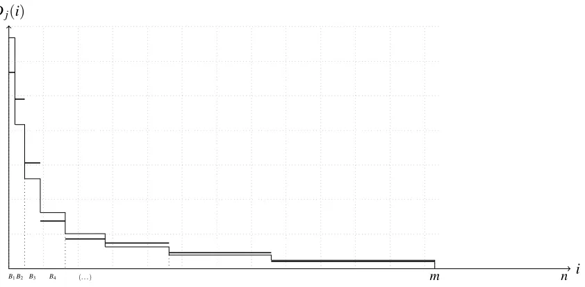
B1B2 B3 B4 (. . .)
Dj(i)
i
m n
Figure 1: Ano-instance(D1,D2)(before permutation).
We now describe the various steps of the construction in greater detail.
Effective support. BothD1andD2, albeit distributions on[n], will have (common)sparsesupport.
In this stepbwill act as a random scaling factor. The objective of this random scaling is to induce uncertainty in the algorithm’s knowledge of the true support size of the distributions, and to prevent it from leveraging this information to test equivalence. In fact one can verify that the class of distributions induced for a single value ofb, namely all distributions have the same value ofm, then one can distinguish theYandNcases with onlyO(1)conditional queries. The test would (roughly) go as follows. Since |Bi|is known, one can choose a random subsetSof the domain which (with high probability) has no
intersection withBifori≤2r−2, aO(1)size intersection withB2r−1, and aO(ρ)size intersection with
B2r. PerformO(1)conditional queries over the setS, for both distributions. Given these queries, we can
then identify which elements ofSbelong toB2r−1orB2r—namely, those which occur at most once belong
toB2r, and those which occur at least twice belong toB2r−1. In aYinstance, then in both distributions, a
1/2 fraction of queries will belong toB2r−1, whereas in aNinstance, one distribution will have either a
1/4 or 3/4 fraction of queries inB2r−1, allowing us to distinguish the two cases.
Buckets. Our construction is inspired by the lower bound of Canonne, Ron, and Servedio [14, Theorem 8] for the more restrictivePAIRCOND access model. We partition the support into 2r consecutive intervals (henceforth referred to asbuckets)B1, . . . ,B2r, where the size of thei-th bucket isbρi. We note
thatrandρwill be chosen such that∑i2=1r bρi=bn1/4, i. e., the buckets fill the effective support.
Distributions. We output a pair of distributions(D1,D2). Each distribution that we construct is uniform
within any particular bucketBi. In particular, the first distribution assigns the same mass 1/2rto each
bucket. Therefore, points withinBihave the same probability mass 1/2rbρi. For theYcase, the second
distribution is identical to the first. For theN case, we pair buckets in r consecutive bucket-pairs
Π1, . . . ,Πr, withΠi=B2i−1∪B2i. For the second distributionD2, we consider the same buckets asD1,
but repartition the mass 1/r withineachΠi. More precisely, in each pair, one of the buckets gets now
total probability mass 1/4r while the other gets 3/4r (so that the probability of every point is either decreased by a factor 1/2 or increased by 3/2). The choice of which goes up and which goes down is done uniformly and independently at random for each bucket-pair determined by the random choices of theπi.
Random relabeling. The final step of the construction randomly relabels the symbols, namely is a ran-dom injective map from[m]to[n]. This is done to ensure that no information about the individual symbol labels can be used by the algorithm for testing. For example, without this the algorithm can consider a few symbols from the first bucket and distinguish theYandNcases. As mentioned inSection 2.3, for ease of analysis, the randomness in the choice of the permutation is, in some sense, deferred to the randomness in the choice ofΛi during the algorithm’s execution.
Summary. Ano-instance(D1,D2)is thus defined by the following parameters: the support sizem,
the vector(π1, . . . ,πr)∈ {0,1}r(which only impactsD2), and the final permutationσ of the domain. A
yes-instance(D1,D1)follows an identical process, however,~π has no influence on the final outcome.
SeeFigure 1 for an illustration of such a(D1,D2) when σ is the identity permutation and thus the
Values forρandr. By settingr=logn/(8 logρ) +O(1), we have as desired∑2i=1r |Bi|=mand there
is a factor(1+o(1))n1/4between the height of the first bucketB1and the one of the last,B2r. It remains
to choose the parameterρitself; we shall take it to be 2
√
logn, resulting inr= (1/8)√logn+O(1). (Note
that for the sake of the exposition, we ignore technical details such as the rounding of parameters, e. g., bucket sizes; these can be easily taken care of at the price of cumbersome case analyses, and do not bring much to the argument.)
3.2 Analysis
We now prove our main lower bound, by analyzing the behavior of core adaptive testers (as per Def-inition 2.5) on the familiesYandNfrom the previous section. InSection 3.2.1, we argue that, with high probability, the sizes of the queries performed by the algorithm satisfy some specific properties. Conditioned upon this event, inSection 3.2.2, we show that the algorithm will get similar information from each query, whether it is running on ayes-instance or ano-instance.
Before moving to the heart of the argument, we state the following fact, straightforward from the construction of ourno-instances.
Fact 3.1. For any(D1,D2)drawn fromN, one hasdTV(D1,D2) =1/4.
Moreover, as allowing more queries can only increase the probability of success, we hereafter focus on a core adaptive tester that performs exactlyq= (1/10)√log logn(adaptive) queries; and will show that it can only distinguish betweenyesandno-instances with probabilityo(1).
3.2.1 Banning “bad queries”
As mentioned inSection 3.1, the draw of ayesorno-instance involves a random scaling of the size of the support of the distributions, meant to “blind” the testing algorithm. Recall that a testing algorithm is specified by a decision tree, which at stepi, specifies how many unseen elements from each atom to include in the query ({kiA}) and which previously seen elements to include in the query (setsKi(1),Ki(2), as defined inSection 2.2), where the algorithm’s choice depends on the observed configuration at that time. Note that, using Yao’s Principle (as discussed inSection 2.3), these choices are deterministic for a given configuration—in particular, we can think of all{kAi}andKi(1),Ki(2)in the decision tree as being fixed. In this section, we show that allkAi values satisfy with high probability some particular conditions with respect to the choice of distribution, where the randomness is over the choice of the support size.
First, we recall an observation from [16], though we modify it slightly to apply to configurations on pairs of distributions and we apply a slightly tighter analysis. This essentially limits the number of states an algorithm could be in by a function of how many queries it makes.
Proposition 3.2. The number of nodes in a decision tree corresponding to a q-sample algorithm is at most26q2+1.
Proof. As mentioned in Definition 2.4, an i-configuration can be described using 6i2 bits, resulting in at most 26i2 i-configurations. Since eachi-configuration leads us to some node on thei-th level of
For the sake of the argument, we will introduce a few notions applying to thesizesof query sets: namely, the notions of a number beingsmall, large, or stable, and of a vector beingincomparable. Roughly speaking, a number is small if a uniformly random set of this size does not, in expectation, hit the largest bucketB2r—in other words, the set is likely to be disjoint from the support. On the other hand,
it is large if we expect such a set to intersect many bucket-pairs (i. e., a significant fraction of the support). The definition of stable numbers is slightly more quantitative: a numberβ is stable if a random set
of sizeβ, for each bucketBi, is either disjoint fromBior has an intersection withBiof size close to the
expected value. In the latter case, we say the setconcentratesoverBi. Finally, a vector of values(βj)is
incomparable if the union of random setsS1, . . . ,Smof sizesβ1, . . . ,βmcontains (with high probability)
an amount of massD S
jSj
which is either much smaller or much larger than the probabilityD(s)of any single elements.
We formalize these concepts in the definitions below. To motivate them, it will be useful to bear in mind that, from the construction described inSection 3.1, the expected intersection of a uniform random set of sizeβ with a bucketBiis of sizeβbρi/n; while the expected probability mass fromBiit contains (under
eitherD1orD2) isβ/2rn.
Definition 3.3. Letqbe an integer, and letϕ=Θ(q5/2). A numberβ is said to besmallifβ<n/(bρ2r);
it islarge(with relation to some integerq) ifβ≥n/(bρ2r−2ϕ).
Note that the latter condition equivalently means that, in expectation, a set of large size will intersect at leastϕ+1 bucket-pairs (as it hits an expected 2ϕ+1 buckets, sinceβB2r−2ϕ
/n≥1). From the
above definitions we get that, with high probability, a random set of any fixed size will in expectation either hit many or no buckets.
Proposition 3.4. A number is either small or large with probability1−O
ϕlogρ
logn
.
Proof. A numberβ is neither large nor small if
ρ2ϕn
β ρ2r ≤b≤
n
β ρ2r.
The ratio of the endpoints of the interval isρ2ϕ. Sinceb=2kb, this implies that at most logρ2ϕ=2
ϕlogρ
values ofkbcould result in a fixed number falling in this range. As there areΘ(logn)values forkb, the
proposition follows.
The next definition characterizes the sizes of query sets for which the expected intersection with any bucket is either close to 0 (less than 1/α, for some thresholdα), or very big (more thanα). (It will be
helpful to keep in mind that we will eventually use this definition withα=poly(q).)
Definition 3.5. A numberβ is said to beα-stable(forα≥1) if, for each j∈[2r],
β ∈/
n
αbρj,
αn
bρj
.
Proposition 3.6. A number isα-stable with probability1−O
rlogα
logn
.
Proof. Fix some j∈[2r]. A numberβ does not satisfy the definition ofα-stability for this jif
n
α β ρj ≤b≤
nα
β ρj.
Sinceb=2kb, this implies that at most log 2α values ofk
bcould result in a fixed number falling in this
range. Noting that there areΘ(logn)values forkband taking a union bound over all 2rvalues for j, the
proposition follows.
The following definition characterizes the sizes of query sets which have a probability mass far from the probability mass of any individual element. (For the sake of building intuition, the reader may replace
νin the following by the parameterbof the distribution.)
Definition 3.7. A vector of numbers(β1, . . . ,β`)is said to be(α,τ)-incomparable with respect toν(for τ≥1) if the two following conditions hold.
• (β1, . . . ,β`)isα-stable.
• Let∆j be the minimum∆∈ {0, . . . ,2r}such that βjν ρ2r−∆
n ≤
1
α,
or 2rif no such∆exists. For alli∈[2r],
1 2rn
`
∑
j=1
βj∆j6∈
1
τ2rν ρi, τ
2rν ρi
.
Recall from the definition ofα-stability of a number that a random set of this size either has essentially
no intersection with a bucket or “concentrates over it” (i. e., with high probability, the probability mass contained in the intersection with this bucket is very close to the expected value). The above definition roughly captures the following. For any j,∆jis the number of buckets that will concentrate over a random
set of sizeβj. The last condition asks that the total probability mass fromD1 (orD2) enclosed in the
union ofmrandom sets of sizeβ1, . . . ,β`be a multiplicative factor ofτ from the individual probability
weight 1/2rbρi of a single element from any of the 2rbuckets.
Proposition 3.8. Given that a vector of numbers of length`isα-stable, it is(α,q2)-incomparable with
respect to b with probability at least
1−O
rlogq logn
.
Proof. Fix any vector(β1, . . . ,β`). By the definition above, for each valuebsuch that(β1, . . . ,β`)is α-stable, we have
βj· α ρ2r
n ≤
ρ∆j b <βj·
α ρ2r+1
or, equivalently,
logα βj
n
logρ +2r+
logb logρ
≤∆j<
logα βj
n
logρ +2r+
logb
logρ+1, j
∈[`].
Writing
λj
def
= log
α βj
n
logρ +2r
for j∈[`], we obtain that
`
∑
j=1
βj∆jb=b
`
∑
j=1
βj(λj+O(1)) +
blogb logρ
`
∑
j=1
βj. (3.1)
• If it is the case that
logρ· `
∑
j=1
βj(λj+O(1))logb·
`
∑
j=1
βj.
Then, for any fixedi∈[2r], to meet the second item of the definition of incomparability we need
`
∑
j=1
βj∆jb∈/[n/(200qρi),200qn/ρi].
This is essentially, with the assumptionequation (3.1)above, requiring that
blogb∈/
"
nlogρ
2q2ρi
∑`j=1βj
,2q
2nlog
ρ
ρi∑`j=1βj
#
.
Recalling thatblogb=kb2kb, this means thatO(logq/log logq)values ofkbare to be ruled out.
(Observe that this is the number of possible “bad values” forbwithout the condition from the case distinction above; since we add an extra constraint onb, there are at most this many values to avoid.)
• Conversely, if logρ·∑`j=1βj(λj+O(1))logb·∑`j=1βjthe requirement becomes
b∈/
"
nlogρ
2q2ρi
∑`j=1βj(λj+O(1))
, 2q
2nlog
ρ
ρi∑`j=1βj(λj+O(1))
#
,
ruling out this timeO(logq)values forkb.
• Finally, the two terms are comparable only if
logb=Θ
logρ·
`
∑
j=1
βj(λj+O(1))·
`
∑
j=1
βj
!−1
;
A union bound over the 2rpossible values ofi, and the fact thatkbcan takeΘ(logn)values, complete the
proof.
We put these together to obtain the following lemma.
Lemma 3.9. With probability at least
1−O 2
6q2+q
(rlogα+ϕlogρ) +26q2(rlogq)
logn
!
,
the following holds for the decision tree corresponding to a q-query algorithm:
• the size of each atom isα-stable and either large or small;
• the size of each atom, after excluding elements we have previously observed,8 isα-stable and either large or small;
• for each i, the vector(kA
i)A∈At(A1,...,Ai)is(α,q
2)-incomparable (with respect to b).
Proof. From Proposition 3.2, there are at most 26q2+1 tree nodes, each of which contains one vector
(kA
i )A, and at most 2qatom sizes. The first point follows fromProposition 3.4andProposition 3.6and
applying the union bound over all 26q2+1·2·2qsizes, where we note the additional factor of 2 comes from either including or excluding the old elements. The latter point follows fromProposition 3.8and applying the union bound over all 26q2+1nodes in the tree (each containing a singlekiAvector).
3.2.2 Key lemma: Bounding the variation distance between decision trees
In this section, we prove a key lemma on the variation distance between the distribution on leaves of any decision tree, when given access to either an instance fromYorN. This lemma will in turn directly yieldTheorem 1.1. Hereafter, we set the parametersα (the threshold for stability),ϕ (the parameter for smallness and largeness) andγ(an accuracy parameter for how well things concentrate over their expected
value) as follows.9 αdef=q7,ϕdef=q5/2andγdef=1/ϕ=q−5/2. (Recall further thatq= (1/10)
√
log logn.)
Lemma 3.10. Conditioned on the events ofLemma 3.9, consider the distribution over leaves of any decision tree corresponding to a q-query adaptive algorithm when the algorithm is given ayes-instance, and when it is given ano-instance. These two distributions have total variation distance o(1).
Proof. This proof is by induction on 1≤i≤q. We will have three inductive hypotheses,EEE111(t),EEE222(t),
andEEE333(t). Assuming all three hold for allt<i, we proveEEE111(i). Additionally assumingEEE111(i), we prove
E E
E222(i)andEEE333(i).
Roughly, the first inductive hypothesis states that the query sets behave similarly to as if we had picked a random set of that size. It also implies that whether or not we get an element we have seen before
8More precisely, we mean to say that for eachi≤q, for every atomAdefined by the partition of(A1, . . . ,A
i), the valueskAi and|A\ {s(11),s(12), . . . ,si(−1)1,s(i−2)1}| −kA
i areα-stable and either large or small.
9This choice of parameters is not completely arbitrary: combined with the setting ofq,rand
ρ, they ensure a total boundo(1)
is “obvious” based on past observances and the size of the query we perform. The second states that we never observe two distinct elements from the same bucket-pair. The third states that the next sample is distributed similarly in either ayes-instance or ano-instance. Note that this distribution includes both features which our algorithm can observe (i. e., the atom which the sample belongs to and if it collides with a previously seen sample), as well as those which it can not (i. e., which bucket-pair the observed sample belongs to). It is necessary to show the latter, since the bucket-pair a sample belongs to may determine the outcome of future queries.
More precisely, the three inductive hypotheses are as follows:
• EEE111(i): In either ayes-instance or ano-instance, the following occurs: For an atomSin the partition generated by A1, . . . ,Ai, let S0 =S \ {s(1)1 ,s(2)1 , . . . ,s(1)i−1,s(2)i−1}. For every such S0, let `S
0 be the largest index`∈ {0, . . . ,2r}such that|S0|bρ`/n≤1/α, or 0 if no such`exists. We claim that
`S0 ∈ {0, . . . ,2r−ϕ−2} ∪ {2r}, and sayS0 is small if`S
0
=2rand large otherwise. Additionally:
– for j≤`S0, S0∩Bj
=0;
– for j> `S0,S0∩Bj
lies in[1−iγ,1+iγ]
|S0|bρj
n .
Furthermore, let p1andp2be the probability mass contained inΛiandΓi, respectively. Then
p1
p1+p2 ≤O
1 q2
or p2
p1+p2 ≤O
1 q2
(that is, either almost all the probability mass comes from elements which we have not yet observed, or almost all of it comes from previously seen ones).
• EEE222(i): No two elements from the set{s (1) 1 ,s
(2) 1 , . . . ,s
(1)
i ,s
(2)
i }belong to the same bucket-pair.
• EEE333(i): Let Tiyes be the random variable representing the atoms and bucket-pairs10 containing
(s(1)i ,s(2)i ), as well as which of the previous samples they intersect with, when thei-th query is performed on ayes-instance, and defineTinosimilarly forno-instances. Then
dTV Tiyes,T no i
≤O 1/q2+1/ρ+γ+1/ϕ=o(1).
We will show thatEEE111(i)holds with probability 1−O 2iexp(−2γ2α/3)
andEEE222(i)holds with probability
1−O(i/ϕ). Let Tyes be the random variable representing the q-configuration and the bucket-pairs
containing each of the observed samples in ayes-instance, and defineTnosimilarly for ano-instance. We note that this random variable determines which leaf of the decision tree we reach, whichEEE333(q)bounds.
We can then take a union bound over alli∈[q]to upper bound the probability thatEEE111(i)andEEE222(i)do
not hold, and useEEE333(i)and the coupling interpretation of total variation distance to upper bound the
probability thatTiyesandTinoever differ. Any of these “failure” events happens with probability at most
O
2qexp
−2γ
2 α 3 +q 2 ϕ + 1 q+ q
ρ+qγ+
q
ϕ
=o(1)
10If a samples(k)
(from our choice ofα,γ,ϕ). This upper bounds the total variation distance betweenTyesandTno, giving
the desired result.
We proceed with the inductive proofs ofEEE111(i),EEE222(i), andEEE333(i), noting that the base cases hold
trivially for all three of these statements. Throughout this proof, recall thatΛiis the set of unseen support
elements which we query, andΓiis the set of previously seen support elements which we query.
Lemma 3.11. Assume that EEE111(t),EEE222(t),EEE333(t)hold for all1≤t≤i−1. Then EEE111(i)holds with probability
at least
1−O
2iexp
−2γ
2α
3
=1−2i−Ω(q2).
Proof. We start with the first part of EEE111(i) (the statement prior to “Furthermore”). Let S (and the
correspondingS0) be any atom as inEEE111(i). First, we note that`S
0
∈ {0, . . . ,2r−ϕ−2} ∪ {2r}since we
are conditioning onLemma 3.9:|S0|isα-stable and either large or small, which enforces this condition.
Next, supposeS0 is contained in some other atomT generated byA1, . . . ,Ai−1, and let
T0=T\ {s(1)1 ,s(2)1 , . . . ,s(1)i−1,s(2)i−1}.
Since|S0| ≤ |T0|, this implies that`T0 ≤`S0. We argue about|T0∩B
j|for three regimes of j:
• The first case is j≤`T0. By the inductive hypothesis,T0∩Bj =0, so
S0∩Bj
=0 with probability
1.
• The next case is`T0< j≤`S0. Recall from the definition of a core adaptive tester thatS0 will be chosen uniformly at random from all subsets ofT0of appropriate size. By the inductive hypothesis,
T0∩Bj
|T0| ∈[1−(i−1)γ,1+ (i−1)γ]
bρj
n , and therefore
ES0∩Bj
∈[1−(i−1)γ,1+ (i−1)γ]|S
0|b
ρj
n , implying E
S0∩Bj
≤ 2
α ρ`S
0 −j;
where the inequality is by the definition of `S0 and using the fact that (i−1)γ ≤1. Using a
Chernoff bound for hypergeometric random variables (Lemma 2.7), and writingµdef=ES0∩Bj
for conciseness,
Pr S0∩Bj
≥1 =Pr S0∩Bj
≥
1+1−µ
µ µ ≤exp
−(1−µ) 2 3µ ≤exp −1
12α ρ
`S0−j
,
where the second inequality holds becauseµ≤2/α ρ`S
0
−jand(1−
µ)2≥1/2 fornsufficiently
• The final case is j> `S0. As in the previous one,
ES0∩Bj
∈[1−(i−1)γ,1+ (i−1)γ]|S
0|b
ρj
n , implying E
S0∩Bj
≥α ρ
j−`S0−1
2 ;
where the inequality is by the definition of`S0,α-stability, and using the fact that(i−1)γ≤1/2.
Using again a Chernoff bound for hypergeometric random variables (Lemma 2.7),
Pr
S0∩Bj
−E
S0∩Bj
≥γ
|S0|bρj
n
≤Pr S0∩Bj
−E
S0∩Bj
≥γ2ES0∩Bj
≤2 exp −(2γ) 2
ES0∩Bj
3
!
≤2 exp
−2
3γ
2
α ρj−`
S0−1
,
where the first inequality comes from 2(1−(i−1)γ)≥1, the second is from Chernoff bound, and
the third follows fromES0∩Bj
≥α ρj−`S
0 −1/2.
Since we wish to prove the statement for all bucketsBjsimultaneously, we take a union bound over all j.
Recall that we want to bound the probability thatS0satisfies two conditions, for j≤`S0, S0∩Bj
=0;
and for j> `S0,S0∩Bj
lies in
[1−iγ,1+iγ]|S
0|b
ρj
n .
Using bounds from all three of these regimes of j, and a union bound, the probability thatS0does not satisfy the conditions ofEEE111(i)is at most
∑
j≤`T0
0+
∑
`T0<j≤`S0 exp
− 1
12α ρ
`S0−j
+
∑
j>`S0 2 exp
−2
3γ
2
α ρj−`
S0−1
.
This probability is maximized when`S0 =`T0 =0, in which case it is
2r
∑
j=1 2 exp −2 3γ 2α ρj−1
≤ ∞
∑
j=1 2 exp −2 3γ 2α ρj−1
≤3 exp
−2 3γ 2 α .
Taking a union bound over at most 2isets gives us the desired probability bound.
Finally, we prove the remainder ofEEE111(i)(the statement following “Furthermore”); this will follow
from the definition of incomparability (Definition 3.7).
• First, we focus onΓi. Suppose thatΓicontains at least one element with positive probability mass
Γi. Since our inductive hypothesis implies thatΓi has no elements in the same bucket pair, the
maximum possible value for p2is
p2≤p02+
3p02
ρ +
3p02
ρ3 +
· · · ≤p02+3p 0
2
ρ
∞
∑
k=0
1
ρ2k =
1+3
ρ
ρ2
ρ2−1
p02
≤(1+o(1))p02.
Therefore,p2∈[p02,(1+o(1))p02]. Supposing this heaviest element belongs to bucket j, we can
say that
p2∈
1
2,(1+o(1)) 3 2
1 2rbρj.
• Next, we focus onΛi. Consider some atomA, from which we selectedkA elements which have
not been previously observed: call the set of these elementsA0. In the first part of this proof, we showed that for each bucketBk, either|A0∩Bk|=0 or|A0∩Bk| ∈[1−iγ,1+iγ]|A0|bρk/n. In the
latter case, noting thatiγ≤1/2 and that the probability of an individual element inBkis within
[1,3] 1 4rbρk,
the probability mass contained by|A0∩Bk|belongs to
[1,9]|A 0|
8rn.
Recalling the definition of∆Aas stated inDefinition 3.7, as shown earlier in this proof, this
non-empty intersection happens for exactly∆Abuckets. Therefore, the total probability mass inΛiis in
the interval
1 4,
9 4
1
2rnA∈At(
∑
A 1,...,Ai)kiA∆A.
Recall that we are conditioning onLemma 3.9which states that the vector(kA
i )A∈At(A1,...,Ai)is(α,q
2)
-incomparable with respect tob. Applying this definition to the bounds just obtained on the probability masses inΛiandΓigivesLemma 3.11.
Lemma 3.12. Assume that EEE111(t),EEE222(t),EEE333(t)hold for all1≤t≤i−1, and additionally EEE111(i)holds.
Then EEE222(i)holds with probability at least1−O(i/ϕ).
Proof. We focus ons(1)i . Ifs(1)i ∈Γi, the conclusion is trivial, so supposes(1)i ∈Λi. FromEEE111(i), no small
atom intersects any of the buckets, so let us condition on the fact thats(1)i belongs to some large atom S. Since we wants(1)i to fall in a distinct bucket-pair from 2(i−1) +1 other samples, there are at most 2i−1 bucket-pairs whichs(1)i should not land in. UsingEEE111(i), the maximum probability mass contained
in the intersection of these bucket-pairs andSis(1+iγ)(2i−1)|S|/rn. Similarly, using the definition of
two terms gives an upper bound on the probability of breaking this invariant, conditioned on landing inS, asO(i/ϕ), where we note that
1+iγ
1−iγ =O(1).
Since the choice of which large atom was arbitrary, we can remove the conditioning. Taking a union bound fors(1)i ands(2)i gives the result.
Lemma 3.13. Assume that EEE111(t),EEE222(t),EEE333(t)hold for all1≤t≤i−1, and additionally EEE111(i)holds.
Then EEE333(i)holds.
Proof. We fix some setting of the intersection history, i. e., the configuration and the bucket-pairs the past elements belong to, and show that the results of the next query will behave similarly, whether the instance is ayes-instance or ano-instance. We note that, since we are assuming the inductive hypotheses hold, certain settings which violate these hypotheses are not allowed. We also note thats(1)i is distributed
identically in both instances, so we focus onsi
def
=s(2)i for the remainder of this proof.
First, we condition that, based on the setting of the past history,siwill either come fromΛiorΓi—this
event happens with probability 1−O 1/q2.
Proposition 3.14. In either ayes-instance or ano-instance, siwill either come fromΛiwith probability
1−O 1/q2, orΓi with probability1−O 1/q2
, where the choice of which one is deterministic based on the fixed configuration and choice for the bucket-pairs of previously seen elements.
Proof. This is simply a rephrasing of the portion ofEEE111(i)following “Furthermore.”
We now try to bound the total variation distance betweenTiyesandTinoconditioning on this event. In the case when it does not hold, we trivially bound the total variation distance by 1, incurring a cost of O 1/q2to the total variation distance between the unconditioned variables. Since our target was for this quantity wasO 1/q2+1/ρ+γ+1/ϕ, it remains to show, in the conditioned space, that the total
variation distance in either case is at mostO(1/ρ+γ+1/ϕ) =O(1/q5/2). We break this into two cases,
the first being whenscomes fromΓi. In this case, we incur a cost in total variation distance which is
O(1/ρ):
Proposition 3.15. In either ayes-instance or ano-instance, condition that sicomes fromΓi. Then one of
the following holds:
• |Γi∩Bj|=0for all j∈[2r], in which case si is distributed uniformly at random from the elements
ofΓi;
• or|Γi∩Bj| 6=0for some j∈[2r], in which case siwill be equal to some s∈Γi with probability
1−O(1/ρ), where the choice of s is deterministic based on the fixed configuration and choice for