A modified DDF-based super-efficiency model handling negative data

Elnaz Babazadeh

Department of Applied Mathematics

Azarbaijan Shahid Madani University, Tabriz, Iran [email protected]

[email protected]

Jafar Pourmahmoud

Department of Applied Mathematics

Azarbaijan Shahid Madani University, Tabriz, Iran [email protected]

Abstract

In conventional DEA models, inputs and outputs are assumed to be non-negative while negative data may occur in some DEA application such as the performance analysis of socially responsible and mutual funds; and the macroeconomic performance where “rate of growth of GDP per capita” can be either negative or positive. To handle the negative data and provide a measure of efficiency for all units, many researches have been studied. In this paper, the radial super-efficiency model based on Directional Distance Function (DDF) is modified to provide a complete ranking order of the DMUs (including efficient and inefficient ones). The proposed model shows more reliability on differentiating efficient DMUs from inefficient ones via a new super-efficiency measure. The properties of proposed model include feasibility, monotonicity and unit invariance. Moreover, the model can produce positive outputs when data are non-negative. Apart from numerical examples, an empirical study in bank sector demonstrates the superiority of the proposed model.

Keywords: Data envelopment analysis; Super-efficiency; Negative data; DDF model.

1. Introduction

Data Envelopment Analysis (DEA) is a powerful tool in the context of production management for performance measurement. The purpose of DEA is to measure the relative efficiency of a set of decision making units (DMUs) where multiple inputs convert into multiple outputs (Charneset al. (1978)). Conventional DEA models assume non-negative values for inputs and outputs. However, there are many applications in which one or more inputs and/or outputs are necessarily negative such as the performance analysis of socially responsible and mutual funds (Basso & Funari (2014)), and the macroeconomic performance where “rate of growth of GDP per capita” can be either negative or positive (Lovell(1995)).In DEA literature, there have been various approaches for dealing with unrestricted in sign variables.

Silva Portelaet al. (2004) proposed range directional measure (RDM) model using some variations of the DDF. Sharp et al. (2007) extended a modified slack-based measure for negative data inspired by the Silva’s RDM model. Emrouznejadet al. (2010) proposed a Semi-Oriented Radial Measure (SORM). While Kerstens and Van de Woestyne (2011) modified the traditional proportional distance function, Cheng et al. (2013) suggested variant of the traditional input- or output-oriented radial efficiency measure to handle negative inputs and outputs. Kerstens and Van de Woestyne (2014) highlighted some shortcomings in Cheng’s method using a more general case of the DDF proposed by Kerstens and Van de Woestyne (2011). An overview of the many DEA modeling approaches can be found in Pastor and Aparicio (2015).

The super-efficiency procedure presents the possible capability of an efficient DMU in expanding its inputs and/or reducing its outputs without becoming inefficient (Chen, Du, & Hoa (2013)). Banker and Chang (2006)exploited the super-efficiency model to detect and remove the outliers. Further, the super-efficiency DEA approach can be viewed as atool for sensitivity analysis where a DMU under evaluation is excluded from reference set (see, e.g., Rousseau & Semple (1995); and Zhu(2001)).

Whereas, in the absence of negative data, the classical super-efficiency model under constant returns to scale (CRS) does not suffer from the infeasibility problem1,the super-efficiency model based upon the variable returns to scale (VRS) may be infeasible for a given DMU under evaluation (see, e.g., Chen & Liang(2011), Lee et al.(2011) and Lee & Zhu (2012)).Many modified VRS radial super-efficiency DEA models were proposed to address the infeasibility issue (see, e.g., Cook et al.(2009), Leeet al.(2011)). On the other hand, Ray (2008) suggested the VRS Nerlove-Luenberger super-efficiency DEA model, based on the DDF model and showed that apart from two exceptions the model is feasible. By choosing proper directions, Chen et al. (2013) proposed a DDF-based VRS super-efficiency DEA model to address the infeasibility issue in the two exceptions. Lin and Chen (2015) considered the model in Chen et al. (2013) when zero data exist in outputs. All these modified super-efficiency DEA models are proposed for the non-negative data and the infeasibility issue when there are non-negative inputs or outputs still exists. In 2013, for the first time, Hadi-Vencheh and Esmaeilzadeh (2013) provided a super-efficiency model based on the RDM model (VE model) for ranking DMUs in the presence of negative data. However, Pourmahmoud et al. (2016) highlighted some shortcomings in VE model and proved the model suffers from the common infeasibility and unboundedness problems. Recently, Lin and Chen (2017) proposed a novel DDF-based VRS radial super-efficiency DEA model which is feasible and is able to handle negative data. They claimed that their proposed model can provide a measure of efficiency for all DMUs in the presence of negative data. This paper highlights some cases that their model is not responding for ranking of DMUs for example when DMUs consume the same inputs. Apart from Hadi-Vencheh and Esmaeilzadeh (2013), and Lin and Chen (2017), super-efficiency models with negative data have received no attention in the literature. The contribution of this paper is fivefold:

1. A modified DDF based super-efficiency model interacting with negative data is proposed.

2. The proposed model is always feasible and conveys good properties such as unit invariance, monotonicity, and providing positive outputs when data are non-negative.

3. The proposed model can provide a ranking order for all DMUs via a new super-efficiency measure and produce improved targets for inefficient units.

4. By using different changing rates for inputs and outputs in the proposed model, DMU reaches the frontier with maximum potential in inputs and outputs.

5. This study shows that in distinguishing DMUs to efficient and inefficient ones, proposed model shows higher reliability than the other super-efficiency model compared in this study.

The rest of the paper is outlined as follows. Section 2 briefly presents the concept of DDF,DDF-based super-efficiency model and the model proposed by Lin and Chen (2017). In Section 3, a modified DDF-based super-efficiency model handling negative data is introduced. In section 4, the proposed model is applied to a numerical example. The penultimate section is devoted to an illustration application and finally Section 6 concludes this study.

2. Preliminaries 2.1. DDF model

Consider a set of n observed DMUs, {𝐷𝑀𝑈_𝑗 (𝑗 = 1,2, … , 𝑛)} where each observation transforms m inputs,𝑥_𝑖𝑗 (𝑖 = 1,2, … , 𝑚), into outputs, 𝑦_𝑟𝑗 (𝑟 = 1,2, … , 𝑠). Consider an input-output bundle of 𝐷𝑀𝑈_𝑜(𝑥_𝑜, 𝑦_𝑜) and a reference input-output bundle(𝑔𝑥, 𝑔𝑦). Furthermore, assume that all data are non-negative. Production possibility set 𝑇𝑜(𝑥, 𝑦)

from the observed input-output for n DMUs can be defined as follows:

𝑇_𝑜(𝑥, 𝑦) = {(𝑥, 𝑦): 𝑥 ≥ ∑ 𝜆_𝑗𝑥_𝑗; 𝑦 ≤ ∑ 𝜆_𝑗𝑦_𝑗; ∑ 𝜆_𝑗 = 1

𝑛

𝑗=1

; 𝜆_𝑗 ≥ 0; (𝑗 = 1,2, … , 𝑛)

𝑛

𝑗=1 𝑛

𝑗=1

}

which is constructed assuming convexity, free disposibility of inputs and outputs, and VRS.

Based on 𝑇𝑜, the DDF regarding 𝑇𝑜(𝑥, 𝑦) can be expressed as follows (Chambers et

al.(1996)):

𝐷(𝑥_𝑜, 𝑦_𝑜; 𝑔𝑥_{, 𝑔}𝑦_{) = max 𝛽 : (𝑥}

𝑜− 𝑔𝑥, 𝑦𝑜+ 𝑔𝑦) ∈ 𝑇𝑜. (1)

The reference bundle (𝑔𝑥, 𝑔𝑦) can be chosen in an arbitrary way and this makes the DDF varies with reference to the evaluated DMU. The VRS DEA formulation for model (1) is as follows:

𝑚𝑎𝑥 𝛽

𝑠. 𝑡. ∑ 𝜆𝑗𝑥𝑖𝑗 ≤ 𝑥𝑖𝑜 − 𝛽𝑔𝑥 𝑛

𝑗=1

, i = 1, 2, … , m,

∑ 𝜆_𝑗𝑦_𝑟𝑗 ≥ 𝑦_𝑟𝑜+ 𝛽𝑔𝑦 𝑛

𝑗=1

, r = 1, 2, … , s,

∑ 𝜆_𝑗 = 1

𝑛

𝑗=1

,

𝜆_𝑗 ≥ 0, j = 1, 2, … , n..

Model (2) combines the features of both an input- and output-oriented models in which each input and output of the unit under assessment are decreased and increased respectively, at the same time by the same portion β.The factor 𝛽∗as the optimal value of βin model (2) is the Nerlove–Luenberger (N–L) measure of technical inefficiency for the evaluated DMU. By implication, its efficiency equals 1 − 𝛽∗ (Ray (2008)).

2.2. Super-efficiency model based on DDF

The idea behind the super-efficiency method is that a DMU under analysis is excluded from the reference set so that the efficientDMUs can receive scores greater than or equal to the unity while the score for the inefficient DMUs do not change. In so doing, the super-efficiency version of model (1) is obtained when DMUounder evaluation is

removed from the reference set.𝑇_𝑜𝑠(𝑥, 𝑦) of super-efficiency for nDMUs can be defined as follows:

𝑇𝑜𝑠(𝑥, 𝑦) =

{

(𝑥, 𝑦): 𝑥

≥ ∑ 𝜆_𝑗𝑥_𝑗; 𝑦 ≤ ∑ 𝜆_𝑗𝑦_𝑗; ∑ 𝜆_𝑗 = 1

𝑛

𝑗=1 𝑗≠𝑜

; 𝜆_𝑗 ≥ 0; (𝑗 = 1,2, … , 𝑛; 𝑗 ≠ 𝑜)

𝑛

𝑗=1 𝑗≠𝑜 𝑛

𝑗=1

𝑗≠𝑜 _}

The super-efficiency based on DDF model (Model (1)) is as follows:

𝐷(𝑥_𝑜, 𝑦_𝑜; 𝑔𝑥_{, 𝑔}𝑦_{) = max 𝛽 : (𝑥}

𝑜− 𝑔𝑥, 𝑦𝑜+ 𝑔𝑦) ∈ 𝑇𝑜𝑠.

DDF-based super-efficiency DEA model can be established as follows:

max 𝛽

s. t. ∑ λjxij ≤ xio− 𝛽𝑔𝑥 n

j=1 j≠o

, i = 1, 2, … , m,

∑n λ_jy_rj ≥ y_ro+ 𝛽𝑔𝑦 j=1

j≠o

, r = 1, 2, … , s,

∑ λj = 1 n

j=1 j≠o

,

λ_j ≥ 0, j = 1, 2, … , n; j ≠ o.

Ray (2008) defined the super-efficiency score of the evaluated DMUo equals1 − 𝛽𝑜∗,

where 𝛽_𝑜∗ is the optimum value of model (3). The smaller the value of 𝛽_𝑜∗, more efficient the DMUo is. For any efficient DMUo, 1 − 𝛽𝑜∗ is no less than 1.

The direction vector (𝑔𝑥, 𝑔𝑦) should be non-negative and non-zero, and can be chosen in anarbitrary way (Chen et al. (2013), Ray (2008)). I fall input and output data are non-negative, the standard DDF for the DMUo is adopted by choosing (𝑥𝑜, 𝑦𝑜) as (𝑔𝑥, 𝑔𝑦)

(Chambers et al. (1998)) and the N-L super-efficiency model (NLS model) is obtained. The NLS model is very often feasible for non-negative data, but it fails in two cases (Ray (2008)). To address these infeasibility issues, Chen et al. (2013) selected a new reference input–output bundle for the DDF and propose a modified DDF-based VRS super-efficiency model. However Lin and Chen (2015) showed that the model proposed by Chen et al. (2013) does not fully eliminate the infeasibility issue in Ray (2008). In this regards, Lin and Chen (2015) proposed a modified DDF-based super-efficiency DEA model (LCS model) by choosing(𝑥𝑖𝑜+ max_j≠o{𝑥𝑖𝑗} , 𝑦𝑟𝑜) as (𝑔𝑥, 𝑔𝑦). The LCS model

successfully addresses the infeasibility issue in conventional VRS radial super-efficiency DEA models and the NLS model under non-negative data.

2.3. Proposed model by Lin and Chen(2017)

Lin and Chen (2017) showed that in the presence of negative data, both the NLS and LCS models might be infeasible. This is because their related direction vectors might be negative, which could result in the DMUo to be further away from the super-efficiency

frontier and thus lead to infeasibility. Accordingly, they choose a new direction vector which is always negative and zero, independent of inputs and outputs being non-negative or not. Their proposed model is as follows:

max 𝛽

s. t. ∑ λjxij n

j=1 j≠o

≤ (1 − 𝛽)xio− 𝑎𝑖𝛽, i = 1, 2, … , m,

∑nj=1λ_jy_rj

j≠o

≥ (1 + 𝛽)y_ro− 𝑏_𝑟𝛽, r = 1, 2, … , s,

∑ λj = 1 n

j=1 j≠o

,

λ_j≥ 0, j = 1, 2, … , n; j ≠ o

(4)

Where𝑎_𝑖 = 𝑘 ∗ max

𝑗=1,2,…,𝑛{|𝑥𝑖𝑗|} , 𝑖 = 1,2, … , 𝑚 and 𝑏𝑟 = min𝑗=1,2,…,𝑛{𝑦𝑟𝑗} , 𝑟 = 1,2, … , 𝑠; k is

a constant, satisfying k ≥ 3.

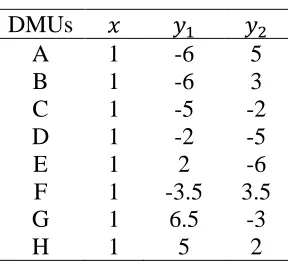
Table 1: Numerical example

DMUs 𝑥 𝑦₁ 𝑦₂

A 1 -6 5

B 1 -6 3

C 1 -5 -2

D 1 -2 -5

E 1 2 -6

F 1 -3.5 3.5

G 1 6.5 -3

H 1 5 2

The results of applying model (4) to the DMUs in Table 1 are presented in Table 2. The optimal values of 1 − 𝛽∗ besides the optimal slack values (s*_;𝑡

1∗,𝑡2∗)are shown in columns

two-five. The input and outputs projections(𝑥∗; 𝑦₁∗, 𝑦₂∗) are represented in the columns six-eight. Projection points are computed by inserting the optimal value in the right-hand side of the input and output inequalities in model (4).

Table 2. The results of numerical example

DMUs 1 − 𝛽∗ s* 𝑡₁∗ 𝑡₂∗ 𝑥∗ 𝑦₁∗ 𝑦₂∗

A 1.1364 0.5455 2.5000 0.0000 1.5455 -6.0000 3.5000

B 1.0000 0.0000 7.3333 0.0000 1.0000 -6.0000 3.0000

C 1.0000 0.0000 10.0000 4.0000 1.0000 -5.0000 -2.0000 D 1.0000 0.0000 7.0000 7.0000 1.0000 -2.0000 -5.0000

E 1.0000 0.0000 3.0000 8.0000 1.0000 2.0000 -6.0000

F 1.0000 0.0000 3.0000 0.0000 1.0000 -3.5000 3.5000

G 1.1200 0.4800 0.0000 5.3600 1.4800 5.0000 -3.3600

H 1.2657 1.0627 0.0000 0.0000 2.0627 2.0776 -0.1254

Table 2 reports that𝛽_𝐵∗ =𝛽_𝐶∗ = 𝛽_𝐷∗ =𝛽_𝐸∗ =𝛽_𝐹∗ = 0,𝛽_𝐴∗ = −0.1364,𝛽_𝐺∗ = −0.1200

and𝛽_𝐻∗ = −0.2657. DMUs A, G and H are Pareto-efficient, while DMUs B, C, D, E and F are inefficient due to the optimal slack-values. Table 1 shows that all the DMUs are on the frontier in their input components meaning that input level is efficient; but due to illogical results for DMUs A, G and H the input projections are not on the efficient frontier, as represented in the sixth column of Table 2. This is because𝑥𝑖𝑜+ 𝑎𝑖 > 0, 𝑖 =

1, 2, … , 𝑚 for each 𝑜 ∈ {1, 2, … , 𝑛} and model (4) uses a unified changing rate 𝛽 for both inputs and outputs. Thus, when DMUs consume the same inputs, our expectation is 𝛽∗ =

3. Proposed super-efficiency model

The single input and both outputs cannot be moved at the same rate to the frontier due to the fact that input level is already efficient, as shown in Table 1. The proposed model by Lin and Chen (2017) is unable to provide a complete ranking order for all the DMUs when DMUs consume the same inputs. Different rates 𝛽_𝑥 and 𝛽_𝑦 should be used for inputs and outputs, respectively. To this end, the proposed model is as follows:

max 𝛽_𝑥+ 𝛽_𝑦

𝑠. 𝑡. ∑ 𝜆_𝑗𝑥_𝑖𝑗

𝑛

𝑗=1 𝑗≠𝑜

≤ 𝑥_𝑖𝑜− (𝑥_𝑖𝑜+ 𝑎_𝑖)𝛽_𝑥, 𝑖 = 1, 2, … , 𝑚,

∑𝑛_𝑗=1𝜆_𝑗𝑦_𝑟𝑗

𝑗≠𝑜

≥ 𝑦_𝑟𝑜+ (𝑦_𝑟𝑜 − 𝑏_𝑟)𝛽_𝑦, 𝑟 = 1, 2, … , 𝑠,

𝛽𝑥. 𝛽𝑦 ≥ 0

∑ 𝜆_𝑗 = 1

𝑛

𝑗=1 𝑗≠𝑜

,

𝜆𝑗 ≥ 0, j = 1, 2, … , n; j ≠ o

(5)

In order to the evaluated DMU reach to the super-efficiency frontier, following conditions are required. If DMUo is efficient, inputs should be increased and outputs

should be contracted, which means 𝛽𝑥 ≤ 0and𝛽𝑦 ≤ 0. And if DMUo is inefficient, inputs

should be contracted and outputs should be increased, which means𝛽_𝑥 ≥ 0and𝛽_𝑦 ≥ 0. These conditions are incorporated by enforcing 𝛽_𝑥. 𝛽_𝑦 ≥ 0 into the model (5). Due to the constraint of 𝛽_𝑥. 𝛽_𝑦 ≥ 0, model (5) is a non-linear programming problem. This non-linear programming problem can be transformed to a linear programming problem using the following procedure. Two binary variables, w and z are introduced and the non-linear constraint 𝛽_𝑥. 𝛽_𝑦≥ 0is transformed into a set of linear constraints as follows:

−𝑀(1 − 𝑤) ≤ 𝛽_𝑥≤ 𝑀𝑤 −𝑀𝑧 ≤ 𝛽_𝑦 ≤ 𝑀(1 − 𝑧) 𝑧 + 𝑤 = 1, 𝑧 ∈ {0,1}, 𝑤 ∈ {0,1}

where M is a sufficiently large number. Obviously, w=1 and z=0 signify 𝛽𝑥≥ 0and𝛽𝑦≥

0, respectively; and w=0 and z=1 signify 𝛽_𝑥 ≤ 0 and 𝛽_𝑦≤ 0, respectively. By substitution of this set of the linear constraints for 𝛽_𝑥. 𝛽_𝑦 ≥ 0, model (5) becomes a mixed integer linear programming problem. When the evaluated DMU moves simultaneously to the frontier through direction of 𝛽_𝑥and 𝛽_𝑦, the non-zero slacks may be survived. To verify the existence of non-zero slack(s), a non-Archimedean infinitesimal with sum of slacks is incorporated into the objective function of model (5) to reflect the optimal slack calculation process in the standard DEA model.

Proposition 1.Model (5) is always feasible and the following inequalities are hold: a) 0 ≤ 𝛽_𝑥∗ < 1and0 ≤ 𝛽_𝑦∗for (𝑥_𝑖𝑜, 𝑦_𝑟𝑜) ∈ 𝑇_𝑜𝑠;and also

b) −1 ≤ 𝛽_𝑥∗ < 0and−1 ≤ 𝛽_𝑦∗ < 0 for(𝑥_𝑖𝑜, 𝑦_𝑟𝑜)𝑇_𝑜𝑠.

Corollary 1.Let 𝛽_𝑥∗ and 𝛽_𝑦∗ be the optimal solutions of model (5), then1−𝛽𝑥

∗

1+𝛽𝑦∗ ≥ 0.

According to corollary 1, the measure of super-efficiency can be defined as following: Definition 1.Let𝜌∗ =1−𝛽𝑥

∗

1+𝛽𝑦∗

2_{, then}

(a) If𝜌∗> 1, then DMUo is an extreme efficient unit.

(b) If 𝜌∗= 1andthe optimal value of the slacks generated by model (5) are zero, then DMUo is a non-extreme efficient unit.

(c) If 𝜌∗ = 1and the optimal value of the slacks produce by model (5) are non-zero, then DMUo is a weak efficient unit.

(d) If 𝜌∗ < 1, then DMUo is an inefficient unit.

From model (5) the output-projections for 𝐷𝑀𝑈𝑜 are

𝑦_𝑟𝑜∗ _{= (1 + 𝛽}

𝑦∗)yro− 𝑏𝑟𝛽𝑦∗ = 𝑦𝑟𝑜 + (𝑦𝑟𝑜− 𝑏𝑟)𝛽𝑦∗, r = 1, 2, … , s

where𝛽_𝑦∗ is the optimal value of model (5).According to Proposition 1,

𝑦𝑟𝑜∗ = 𝑦𝑟𝑜+ (𝑦𝑟𝑜− 𝑏𝑟)𝛽𝑦∗ ≥ 𝑦𝑟𝑜,when(𝑥𝑖𝑜, 𝑦𝑟𝑜) ∈ 𝑇𝑜𝑠 and

𝑦𝑟𝑜∗ = 𝑦𝑟𝑜 + (𝑦𝑟𝑜− 𝑏𝑟)𝛽𝑦∗ ≥ 𝑦𝑟𝑜 − (𝑦𝑟𝑜− 𝑏𝑟) = 𝑏𝑟, when (𝑥𝑖𝑜, 𝑦𝑟𝑜)𝑇𝑜𝑠.∎

Therefore, the following Lemma is hold.

Lemma 2.For the data set with non-negative outputs, 𝑦_𝑟𝑜∗ ≥ 0satisfies for any DMUo

(𝑜 ∈ {1,2, … , 𝑛}).

Corollary 2.If𝛽_𝑥= 𝛽_𝑦 = 𝛽 in model (5), the proposed model is equivalent with the model (4), consequently the conceptual problem described in Ray (2008) does not occur.

Proposition 2. Model (5) is unit invariant. Proof. The proof is given in Appendix B.

Proposition 3.If inputs (outputs) of the DMUo are reduced (increased), the optimal value

of model (5) does not increase.

Proof. The proof is given in Appendix C.

Further examination of the proposed method is made by applying DMUs in Table 1. Table 3 reports the results when proposed model is applied to the numerical example in Table1. The optimal solutions of the proposed model i.e. the optimal values of 𝛽_𝑥∗ and𝛽_𝑦∗ are shown in the second and third columns of Table 3, respectively; and the super-efficiency measure (𝜌∗)is presented in the fourth column. The columns five-seven of Table 3 show the projection point for a DMU under evaluation.

2_{Note that Whenβ}

y

∗ _{= −1, 𝜌}∗ _{diverges to infinity, hence the super-efficiency measure is}

Table 3: The results of applying proposed model for data set in Table 1 (M=100) ranking

order

𝑦₂∗

𝑦₁∗

𝑥∗ 𝜌∗ 𝛽𝑦∗ 𝛽𝑥∗ DMUs 2 3.5000 -6.0000 1.0000 1.1579 -0.1364 0.0000 A 5 5.0000 -6.0000 1.0000 0.8182 0.2222 0.0000 B 7 4.2979 -3.4255 1.0000 0.3884 1.5745 0.0000 C 8 -2.8837 6.4651 1.0000 0.3209 2.1163 0.0000 D 6 -6.0000 6.5000 1.0000 0.6400 0.5625 0.0000 E 4 4.2634 -3.2991 1.0000 0.9256 0.0804 0.0000 F 3 -3.3600 5.0000 1.0000 1.1364 -0.1200 0.0000 G 1 -0.1254 2.0776 1.0000 1.3618 -0.2657 0.0000 H

The results show that DMUs A, G and H are efficient; since their supper-efficiency measures are greater than one. However, DMUs B, C, D, E and F are inefficient, since their supper-efficiency measures are less than one. Using different changing rates for input and outputs, proposed model provides β_x∗ = 0 for all DMUs, unlike the model (4). Column five shows thatx∗ = 1for all the DMUs, and this logical outcome was expected. The proposed model provided ranking order for all the DMUs, shown in column eight:

𝐻 ≻ 𝐴 ≻ 𝐺 ≻ 𝐹 ≻ 𝐵 ≻ 𝐸 ≻ 𝐶 ≻ 𝐷.

4. Numerical example

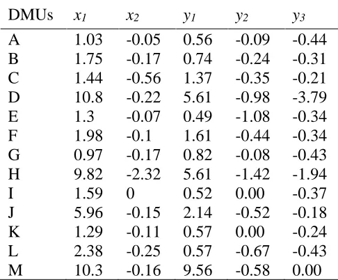
In this section, data set of “the notional effluent processing system” from Sharp et al. (2007) is used to show the applicability and merits of the proposed model.

The data set is presented in Table 4. There are 13 DMUs, with two inputs {x1, x2} and

three outputs {y1, y2, y3}:one positive input (cost), one non-positive input (effluent), one

positive output (saleable output), and two non-positive outputs (methane and CO2).

Table 4: Data sets extracted from Sharp

DMUs x1 x2 y1 y2 y3

A 1.03 -0.05 0.56 -0.09 -0.44

B 1.75 -0.17 0.74 -0.24 -0.31

C 1.44 -0.56 1.37 -0.35 -0.21

D 10.8 -0.22 5.61 -0.98 -3.79

E 1.3 -0.07 0.49 -1.08 -0.34

F 1.98 -0.1 1.61 -0.44 -0.34

G 0.97 -0.17 0.82 -0.08 -0.43

H 9.82 -2.32 5.61 -1.42 -1.94

I 1.59 0 0.52 0.00 -0.37

J 5.96 -0.15 2.14 -0.52 -0.18

K 1.29 -0.11 0.57 0.00 -0.24

L 2.38 -0.25 0.57 -0.67 -0.43

M 10.3 -0.16 9.56 -0.58 0.00

columns four-sixin Table 5, respectively. DMUs C, G, H, K and M are efficient, since their super-efficiency measures are greater than 1. Other DMUs are inefficient, since their supper-efficiency measures are less than 1. The ranking order for DMU M is superior to other DMUs, as shown in the seventh column in Table 5.

Table 5: Applying the proposed model for data set in Table 4(M=100)

Ranking Order 𝜌∗ 𝛽𝑦∗ 𝛽𝑥∗ Ranking Order 1 − 𝛽∗

DMUs 7 0.9866 0.0136 0.0000 7 0.9982 A 9 0.9648 0.0253 0.0108 10 0.9863 B 3 1.0629 0.0000 -0.0629 3 1.0412 C 13 0.5714 0.7501 0.0000 13 0.9192 D 8 0.9713 0.0296 0.0000 8 0.9955 E 10 0.9552 0.0398 0.0068 9 0.9921 F 5 1.0120 0.0000 -0.0120 5 1.0108 G 2 1.4239 0.0000 -0.4239 2 1.4023 H 6 0.9912 0.0000 0.0088 6 1.0000 I 11 0.9482 0.0000 0.0518 11 0.9829 J 4 1.0406 -0.0310 -0.0083 4 1.0292 K 12 0.9132 0.0655 0.0270 12 0.9694 L 1 2.1747 -0.5402 0.0000 1 1.5402 M

As it is shown in the second and the sixth columns in Table 5, both models are feasible for all DMUs and they can differentiate the performance of both efficient and inefficient DMUs for used data set. The ranking orders of both models are close; however their super-efficiency measures are different. This is due to the fact that, in proposed model i.e., model (5) different rates, 𝛽_𝑥 and 𝛽_𝑦 for inputs and outputs respectively are used, while the same rates are used for both inputs and outputs in the model (4). The super-efficiency measure provided by Model (4) for DMU I is 1.0000 however, the measure of

𝜌∗ _{as the measure of super-efficiency yielded by model (5) is 0.9912. This shows that}

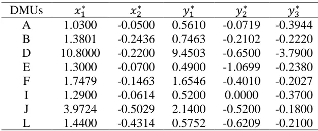
model (5) is more responsive than model (4) and it can differentiate the DMUs more discretely. Table 6 shows the target input-output values of inefficient DMUs, determined by the model (5). The proposed model demonstrates that in each inefficient DMU, the inputs and the outputs should be reduced and expanded, respectively, in order to tend to the super-efficiency frontier. Hence, the proposed model can provide improved target inputs and outputs for all the inefficient DMUs.

Table 6: Improved targets for inefficient DMUs

𝑦₃∗

𝑦₂∗

𝑦₁∗

𝑥₂∗

𝑥₁∗

Lin and Chen (2017) calculated the improved targets for inefficient DMUs. By comparison of their results and the results obtained using proposed model, shown in Table 6, it can be concluded that for some of the DMUs the targets obtained using model (4) is more improved (in some components) than the one obtained using model (5). In other DMUs the proposed model provided more improved targets (in some components) than the model (4). These variations are due to having different directions in their movements to reach the super-efficiency frontier.

5. An empirical application

In this section the proposed model is illustrated by applying it to a real world data of the 61 banks in the GCC3 _{countries. In this evaluation, the input variables are total assets,}

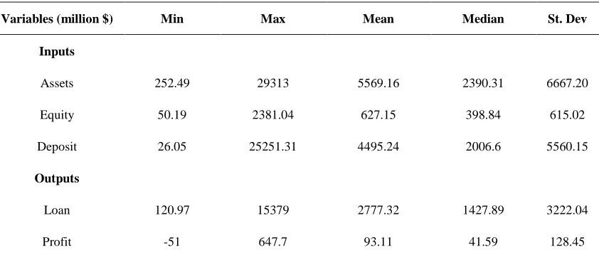
capital and deposits. The output variables are loans and equity in each branch. Note that the last output could take both positive and negative values among the banks. For full definitions of variables see Emrouznejad and Anouze (2010). Table 7 below shows the descriptive statistics of the variables.

Table 7: Descriptive statistics of the banks data

Variables (million $) Min Max Mean Median St. Dev

Inputs

Assets 252.49 29313 5569.16 2390.31 6667.20

Equity 50.19 2381.04 627.15 398.84 615.02

Deposit 26.05 25251.31 4495.24 2006.6 5560.15

Outputs

Loan 120.97 15379 2777.32 1427.89 3222.04

Profit -51 647.7 93.11 41.59 128.45

The outcomes after applying assumed data set in Model (4) and in model (5) are reported in Table 8.

3_{The Gulf Cooperation Council (GCC), is a trade bloc involving the six Arab states of thePersian Gulf with}

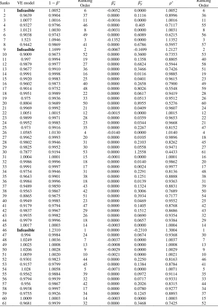
Table 8: Outcomes after applying the assume data on the model (4) and the model (5) (M=100)

Banks VE model 1 − 𝛽∗ Ranking

Order 𝛽𝑥∗ 𝛽𝑦

∗ _𝜌∗ Ranking

Order

1 Infeasible 1.0052 6 -0.0052 0.0000 1.0052 6

2 0.9639 0.9904 37 0.0000 0.1116 0.8996 36

3 1.0077 1.0016 11 -0.0016 0.0000 1.0016 11

4 0.9327 0.9796 46 0.0000 0.405 0.7117 55

5 1.0121 1.0030 8 -0.0031 0.0000 1.0031 8

6 0.9038 0.9743 49 0.0000 0.6089 0.6215 56

7 1.523 1.0946 3 -0.1352 0.0000 1.1352 3

8 0.9442 0.9869 41 0.0000 0.6786 0.5957 57

9 Infeasible 1.1699 2 -0.0067 -0.1699 1.2127 2

10 0.9009 0.9673 52 0.0000 0.3600 0.7353 53

11 0.997 0.9994 19 0.0000 0.1358 0.8805 40

12 0.9879 0.9977 27 0.0000 0.6824 0.5944 58

13 0.9677 0.9910 36 0.0000 0.3466 0.7426 51

14 0.9991 0.9998 16 0.0000 0.0116 0.9885 19

15 0.9920 0.9983 25 0.0000 0.0401 0.9615 23

16 0.9602 0.9873 40 0.0000 0.2658 0.7900 49

17 0.9014 0.9752 48 0.0000 0.8026 0.5548 59

18 0.9951 0.9989 22 0.0000 0.0617 0.9419 28

19 0.975 0.9936 33 0.0000 0.0513 0.9512 26

20 0.8804 0.9689 50 0.0000 0.8955 0.5276 60

21 0.9969 0.9992 21 0.0000 0.0409 0.9607 24

22 1.0051 1.0015 12 -0.0015 0.0000 1.0015 12

23 0.9899 0.9971 28 0.0000 0.0359 0.9653 22

24 0.9952 0.9985 23 0.0000 0.0344 0.9668 21

25 0.973 0.9916 35 0.0000 0.2267 0.8152 47

26 1.0585 1.0130 4 -0.0140 0.0000 1.0140 4

27 0.9962 0.9993 20 0.0000 0.0105 0.9896 18

28 0.9802 0.9946 31 0.0000 0.2103 0.8262 45

29 0.9825 0.9952 30 0.0000 0.0558 0.9471 27

30 0.7877 0.9194 53 0.0000 1.2558 0.4433 61

31 1.0004 1.0001 15 -0.0001 0.0000 1.0001 16

32 0.9986 0.9996 18 0.0000 0.0140 0.9862 20

33 0.9991 0.9997 17 0.0000 0.0024 0.9977 17

34 0.9754 0.9946 31 0.0000 0.2291 0.8136 48

35 0.9643 0.9901 38 0.0000 0.1251 0.8888 38

36 0.9984 0.9996 18 0.0000 0.0139 0.9363 31

37 0.9489 0.9850 43 0.0000 0.1324 0.8831 39

38 0.9563 0.9867 42 0.0000 0.3006 0.7689 50

39 0.8865 0.9675 51 0.0000 0.3934 0.7177 54

40 0.9949 0.9985 23 0.0000 0.0469 0.9552 25

41 0.9179 0.9794 47 0.0000 0.1405 0.8768 42

42 0.9837 0.9967 29 0.0000 0.1512 0.8686 43

43 0.9935 0.9982 26 0.0000 0.0690 0.9354 32

44 0.9979 0.9996 18 0.0000 0.0657 0.9384 29

45 1.0017 1.0003 14 -0.0003 0.0000 1.0004 14

46 Infeasible 1.2310 1 0.0000 -0.2310 1.3004 1

47 0.994 0.9984 24 0.0000 0.0674 0.9368 30

48 1.0249 1.0036 7 -0.0037 0.0000 1.0037 7

49 1.0025 1.0008 13 -0.0008 0.0000 1.0008 13

50 1.0206 1.0028 9 -0.0029 0.0000 1.0029 9

51 1.0059 1.0020 10 -0.0021 0.0000 1.0021 10

52 0.9301 0.9823 44 0.0000 0.2250 0.8163 46

53 0.9157 0.9799 45 0.0000 0.1384 0.8784 41

54 1.028 1.0058 5 -0.0071 0.0000 1.0071 5

55 0.9562 0.9884 39 0.0000 0.0972 0.9114 35

56 0.9794 0.9939 32 0.0000 0.0717 0.9331 33

57 0.956 0.9867 42 0.0000 0.2026 0.8315 44

58 0.9938 0.9997 17 0.0000 0.0780 0.9277 34

59 0.9755 0.9926 34 0.0000 0.1245 0.8893 37

60 1.0009 1.0003 14 -0.0003 0.0000 1.0003 15

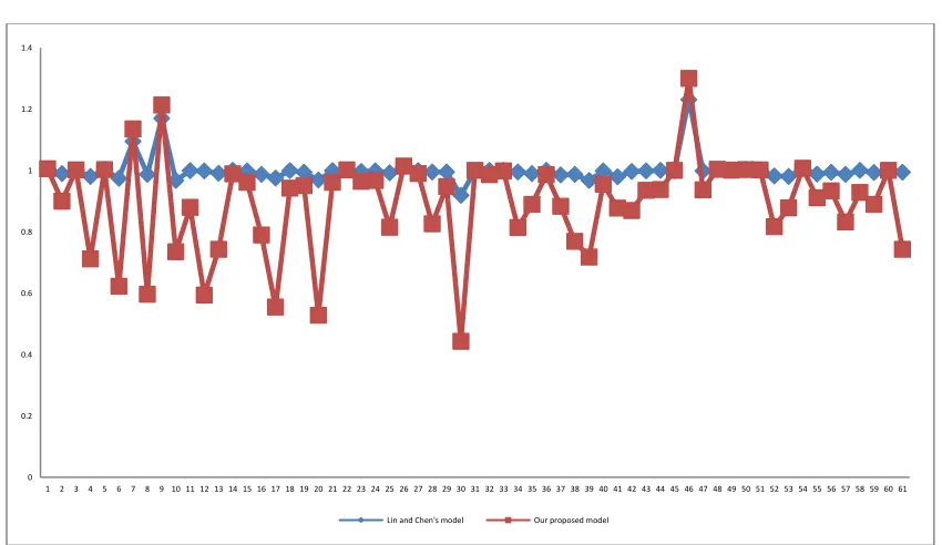
From the second, third and the sixth columns in Table 8, VE model is infeasible for DMUs 1, 9 and 46. Both models (4) and (5) are feasible for all DMUs; however their super-efficiency measures are different. 16 DMUs are found efficient by both models. The super-efficiency measure provided by Model (4) for DMUs 14, 32, 33, 36, 44 and 58 is almost 1.0000 (this is the case when the values are rounded with 3 decimal digits); however the measure of 𝜌∗ as the measure of super-efficiency yielded by proposed model is 0.9885, 0.9862, 0.9977, 0.9863, 0.9384 and 0.9277. The result shows that model (5) is more precise and responsive than model (4) in discriminating the DMUs. From Table 8,all the super-efficiency scores yielded by model (5) for inefficient(efficient) DMUs are less than or equal (bigger than or equal)to those generated by model (4) as shown in Figure 1.Thus, super-efficiency scores vary from 0.9194 to 1.2310 under the Lin and Chen’s model, whereas they vary from 0.4433 to 1.3004 under our proposed model. As can be seen,in general, the super-efficiency scores obtained from model (4) is around 1.0000 for inefficient DMUs, whereas these scores yielded from model (5) have bigger changing ranges for inefficient ones. From Table 8, DMUs 46 and 30 have the best and the worst performance, respectively under both models. Column seven presents a complete ranking order for all DMUs (both efficient and inefficient ones) using proposed model. However, Lin and Chen’s model cannot put discriminations between some inefficient DMUs: between DMUs 45 and 60,DMUs 33 and 58,DMUs 32, 36 and 44,DMUs 24 and 40,DMUs 28 and 34,DMUs 56 and 61,and also DMUs 38 and 57.

Figure 1: Comparison of efficiency score from Lin and Chen’s model and our proposed model.

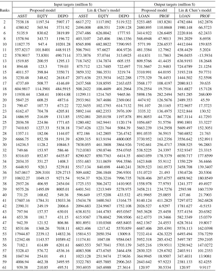
Table 9 shows the target input-output values of inefficient DMUs, determined by both models.

0 0.2 0.4 0.6 0.8 1 1.2 1.4

1 2 3 4 5 6 7 8 9 10 11 12 13 14 15 16 17 18 19 20 21 22 23 24 25 26 27 28 29 30 31 32 33 34 35 36 37 38 39 40 41 42 43 44 45 46 47 48 49 50 51 52 53 54 55 56 57 58 59 60 61

Table 9: Improved targets for inefficient DMUs provided by two models

Banks

Input targets (million $) Output targets (million $) Proposed model Lin & Chen’s model Proposed model Lin & Chen’s model

ASST EQTY DEPO ASST EQTY DEPO LOAN PROF LOAN PROF

2 7538.18 1197.54 5907.17 6617.272 1117.092 5119.522 5253.485 183.8281 4782.684 162.2876 4 4380.82 565.94 3731.92 2496.008 408.551 2109.128 2680.895 110.8868 1980.148 66.5723 6 5135.9 830.62 3819.89 2747.486 626.0042 1777.93 3414.922 126.6405 2220.816 62.2433 8 1578.94 343.73 1196.72 403.3107 245.406 186.1356 568.6948 47.9013 391.2029 8.6938 10 11827.75 947.4 10201.28 8565.898 682.8822 7390.993 5771.99 226.6537 4412.044 159.835 11 557.8217 101.8401 448.9115 506.7941 97.6627 404.9726 481.3384 12.7962 438.4429 5.2024 12 578.9017 73.8301 490.7114 373.3876 57.0744 313.6925 414.831 11.7863 296.0455 -13.5934 13 1519.85 200.55 1295.13 718.7452 134.7874 605.155 809.5766 41.4435 636.9193 18.2648 14 894.68 123.3 739.03 875.712 121.7485 722.697 731.5667 21.9483 724.6789 21.1254 15 4011.57 398.84 3350.71 3859.332 386.3531 3219.74 3310.991 64.0195 3193.218 59.7731 16 3230.48 348.62 2618.47 2071.636 253.3934 1622.288 1775.329 78.4453 1444.502 52.5598 17 4737.69 508.77 4146.69 2437.568 318.8595 2163.655 3568.177 108.4197 2080.813 39.635 18 604.9817 114.3901 484.5915 508.2422 106.4609 401.2964 376.2554 19.7516 361.6827 15.7128 19 11938.44 1268.61 10014.88 11299.11 1214.765 9465.86 5898.156 282.2494 5651.285 268.009 20 5847.25 608.25 4873.6 2933.961 367.4686 2369.061 4474.92 126.5676 2489.353 45.59 21 790.47 107.73 673.22 722.5455 102.1793 614.7132 591.107 20.1165 572.9657 17.3723 23 6162.47 704.78 4205.81 5892.144 682.2353 3976.109 3335.32 136.4975 3232.844 130.52 24 1686.95 216.09 1313.85 1552.081 205.0158 1197.878 891.8053 44.7726 867.3114 41.7293 25 2036.58 224.86 1771.65 1280.482 162.9441 1120.174 1056.687 51.5756 890.1801 33.3227 27 7410.83 1227.33 5138.18 7347.426 1221.764 5084.39 5663.239 154.2958 5609.497 152.3051 28 1357.11 182.06 1144.07 872.186 142.2805 726.4742 891.0535 36.5915 760.6852 21.763 29 6666.75 852.58 5191.39 6209.315 813.9194 4800.005 3730.952 163.2356 3556.642 152.8911 30 16236.5 1128.2 10846.5 7838.055 461.3808 3864.926 7192.661 256.4717 3508.525 96.2883 32 749.66 153.97 586.46 712.0383 150.8746 554.0765 538.5225 24.3397 532.9347 23.3315 33 8316.03 852.87 6435.87 8290.827 850.7763 6414.35 6043.059 178.3379 6030.717 177.8599 34 2034.35 351.27 1408.3 1551.683 311.0659 994.3586 1623.848 55.9112 1350.229 36.4466 35 6448.93 920.3 5239.81 5517.134 840.698 4440.241 3839.523 161.0573 3458.708 139.3407 36 547.0617 209.3101 329.2715 509.4482 206.1848 296.9301 151.0723 21.493 150.6726 20.5304 37 10632.27 1049.15 9271.54 9154.37 926.3216 7996.735 7638.406 207.6757 6858.962 180.8549 38 2937.26 406.95 2454.04 1725.153 306.2472 1410.903 1558.978 77.9793 1241.377 49.4927 39 9575.26 1495.09 8005.01 6401.541 1213.949 5278.975 3458.211 234.7276 2593.98 160.7339 40 731.25 168.62 549.36 596.649 157.5208 433.532 451.9965 25.0855 437.66 21.7903 41 17607.16 1784.31 15033.36 15434.78 1600.563 13164.75 8140.124 411.2825 7297.072 362.6828 42 2390.31 249.19 2006.6 2094.683 224.9967 1752.108 2026.527 6.9297 1781.627 -0.5153 43 797.94 157.57 630.01 638.8151 144.4783 493.0367 565.3628 25.4458 537.4154 20.6382 44 653.38 181.7 431.15 615.9367 178.6042 398.9506 612.4373 19.3466 582.3349 15.0379 47 942.39 121.52 806.86 801.8951 110.0368 685.8403 662.1367 24.4553 628.7614 19.8017 52 8531.06 1368.26 7038.11 6821.406 1217.42 5570.859 6687.406 205.4391 5576.113 162.0398 53 17944.87 2239.12 14832.36 15814.53 2050.354 13009.8 7232.414 426.3225 6493.494 376.7259 55 12342.48 1143.57 10589.42 11174.81 1047.08 9584.043 5952.318 285.4342 5497.787 259.2105 56 7182.1 614.89 6201.61 6603.553 567.7041 5703.139 3455.216 159.9511 3250.942 147.0272 57 5328.43 576.72 4536.16 4083.508 473.6765 3464.458 2830.325 129.6702 2403.911 101.2353 58 1047.94 254.01 49.1 1023.128 251.9474 27.9636 364.9945 18.9507 347.4031 13.9081 59 4006.94 462.38 3495.95 3322.783 405.7885 2906.263 2643.642 97.9223 2381.133 82.4255 61 939.38 210.85 495.51 393.6935 165.6988 27.3614 120.97 30.5334 120.97 9.9117

From the theoretical analyses it is concluded that, the same as Lin and Chen’s model, the proposed model can deal with the data set with free in sign values and can provide improved targets for inefficient DMUs.

6. Conclusion

Conventional DEA models are introduced to evaluate DMUs with non-negative data, while in practice there are important DMUs with negative data and they need to be evaluated. Recently, Lin and Chen (2017) proposed a novel DDF-based VRS radial super-efficiency DEA model which is feasible and is able to handle negative data. They claimed that their proposed model can provide a measure of efficiency for all DMUs. In this study, it is shown that although their proposed model can overcome the common infeasibility problem, the model has failing in some cases. It is unable to provide a complete ranking order and logical results in such a case that all DMUs consume the same inputs. This is because(i) in this model a unified changing rate for both inputs and outputs is used and (ii) the input improvement direction is strictly positive. In this study, a modified radial DDF-based super-efficiency model is proposed to provide a complete ranking order for all the DMUs via a new super-efficiency measure.

References

1. Ali, A.I., & Seiford, L.M., (1990).Translation invariance in data envelopment analysis, Operations Research Letters, 9(6), 403-405.

2. Andersen, P., & Petersen, N.C., (1993).A procedure for ranking efficient units in data envelopment analysis. Management Science, 39 (10), 1261–1294.

3. Banker, R.D., &Chang, H., (2006).The super-efficiency procedure for outlier identification, not for ranking efficient units. European Journal of Operational Research 175,1311–1320.

4. Basso, A., & Funari, S., (2014).Constant and variable returns to scale DEA models for socially responsible investment funds. European Journal of Operational Research, 235(3), 775-783.

5. Chambers, R., Chung, Y., & Färe, R., (1998). Profit, directional distance functions, and Nerlovian efficiency. Journal of Optimization Theory and Applications, 98: 351–364.

6. Chambers, R. G., Chung, Y., & Färe, R., (1996). Benefit and distance functions. Journal of Economic Theory, 70, 407–419

7. Charnes A., Cooper W. W., & Rhodes E., (1978).Measuring the efficiency of decision making units. European Journal of Operational Research, 2(6): 429-444. 8. Chen, Y., Du, J., & Hoa, J., (2013). Super-efficiency based on a modified

directional distance function. Omega, 41, 621-625.

10. Cheng, G., Zervopoulos, P., & Qian, Z., (2013).A variant of radial measure capable of dealing with negative inputs and outputs in data envelopment analysis. European Journal of Operational Research, 225(1), 100–105.

11. Cook, W.D., Liang, L., Zha, Y., & Zhu, J., (2009). A modified super-efficiency DEA model for infeasibility. Journal of Operational Research Society, 60, 276– 281.

12. Emrouznejad, A., Anouze, A. L., & Thanassoulis, E., (2010).A semi-oriented radial measure for measuring the efficiency of decision making units with negative data, using DEA. European Journal of Operational Research 200(1), 297-304.,

13. Emrouznejad, A. & Anouze, A. L., (2010).Data envelopment analysis with classification and regression tree - A case of banking efficiency. Expert Systems with Applications, 27(4): 231-246.

14. Hadi-Vencheh, A., & Esmaeilzadeh, A., (2013).A new super-efficiency model in the presence of negative data. Journal of the Operational Research Society, 64(3), 396-401.

15. Kerstens, K., & Van de Woestyne, I., (2011). Negative data in DEA: a simple proportional distance function approach. Journal of the Operational Research Society, 62(7), 1413-1419.

16. Kerstens, K., & Vande Woestyne, I., (2014).A note on a variant of radial measure capable of dealing with negative inputs and outputs in DEA. European Journal of Operational Research, 234(1), 341-342.

17. Lee, H. S., & Zhu, J., (2012).Super-efficiency infeasibility and zero data in DEA. European Journal of Operational Research, 216, 429–433.

18. Lee, H. S., Chu, C. W., & Zhu, J., (2011).Super-efficiency DEA in the presence of infeasibility. European Journal of Operational Research 212, 141–147.

19. Lin, R., & Chen, Z., (2015). Super-efficiency measurement under variable return to scale: an approach based on a new directional distance function. Journal of the Operational Research Society 66, 1506–1510.

20. Lin, R., & Chen, Z., (2017). A directional distance based super-efficiency DEA model handling negative data. Journal of the Operational Research Society 68(11), 1312-1322.

21. Lovell, C.A.K., (1995), Measuring the Macroeconomic Performance of the Taiwanese Economy. International Journal of Production Economics, 39, 165-178.

22. Pastor, J.T., & Aparicio, J., (2015).Translation Invariance in Data Envelopment Analysis (pp. 245-268).Springer US.

24. Pourmahmoud, J., Hatami-Marbini, A., & Babazadeh, E., (2016).A comment on a new super-efficiency model in the presence of negative data. Journal of the Operational Research Society 67(3), 530-534.

25. Ray, S. C., (2008). The directional distance function and measurement of super-efficiency: an application to airlines data. Journal of the Operational Research Society 59(6), 788-797.

26. Rousseau, J.J., Semple, J.H., (1995). Radii of classification preservation in data envelopment analysis: A case study of 'Program Follow-Through'. Journal of the Operational Research Society 943–957.

27. Silva Portela, M.C.A., Thanassoulis, E., & Simpson, G., (2004). A directional distance approach to deal with negative data in DEA: An application to bank branches. Journal of the Operational Research Society, 55 (10): 1111-1121.

28. Sharp, J. A., Meng, W., & Liu, W., (2007).A modified slacks-based measure model for data envelopment analysis with ‘natural’ negative outputs and inputs. Journal of the Operational Research Society 58(12), 1672-1677.

Appendix A

Proposition 1.Model (5) is always feasible and the following inequalities are hold: a) 0 ≤ 𝛽_𝑥∗ < 1and 0 ≤ 𝛽_𝑦∗for (𝑥_𝑖𝑜, 𝑦_𝑟𝑜) ∈ 𝑇_𝑜𝑠;and also

b) −1 ≤ 𝛽_𝑥∗ < 0and−1 ≤ 𝛽_𝑦∗ < 0 for(𝑥_𝑖𝑜, 𝑦_𝑟𝑜)𝑇_𝑜𝑠.

Proof. Since𝑥_𝑖𝑜+ 𝑎_𝑖 > 0, we have

𝛽𝑥≤

xio−∑nj=1λjxij j≠o

𝑥𝑖𝑜+𝑎𝑖 , 𝑖 = 1,2, … , 𝑚.

(6) Following the notations used by Lin and Chen (2017), let 𝐽𝑜 = {𝑟|𝑦𝑟𝑜 − 𝑏𝑟 > 0, r =

1,2, … , s} and𝑂_𝑜= {𝑟|𝑦_𝑟𝑜− 𝑏_𝑟 = 0, r = 1,2, … , s}for each 𝑜 ∈ {1, 2, … , 𝑛}. Thus, y_ro−

𝑏_𝑟 ≥ 0 implies thatJ_o∪ O_o= {r = 1,2, … , s}. Due to convexity constraint i.e. ∑n_j=1λ_j =

j≠o

1, we have

∑nj=1λ_jy_rj

j≠o

≥ min

j≠o{yrj} ≥ minj {yrj} = br = yro, r ∈ 𝑂𝑜.

This shows that the output constraints in model (5) satisfy for allr ∈ 𝑂_𝑜.Hence, the output constraints in model (5) are equivalent to

𝛽_𝑦 ≤

∑n_j=1λ_jy_rj

j≠o

−yro

yro−𝑏𝑟 , r ∈ 𝐽𝑜.

There are two cases as follows:

(7)

Case (I)when (𝑥_𝑖𝑜, 𝑦_𝑟𝑜) ∈ 𝑇_𝑜𝑠: We have ∑nj=1λjxij

j≠o

≤ xio, 𝑖 = 1, 2, … , 𝑚and∑nj=1λjyrj j≠o

≥ yro, 𝑟 = 1, 2, … , 𝑠. So,

xio− ∑nj=1λjxij j≠o

𝑥𝑖𝑜+ 𝑎𝑖 ≥ 0, 𝑖 = 1, 2, … , 𝑚,

(8)

∑nj=1λjyrj j≠o

−yro

yro−𝑏𝑟 ≥ 0, r ∈ 𝐽𝑜. (9)

Inequalities of (6)-(9) result that 𝛽_𝑥 = 𝛽_𝑦 = 0 is a feasible solution of model (5), and consequently 𝛽𝑥∗≥ 0, and 𝛽𝑦∗ ≥ 0 always hold for 𝑜 ∈ {1, 2, … , 𝑛}. In addition

𝛽𝑥≤

xio−∑nj=1λjxij j≠o

𝑥𝑖𝑜+𝑎𝑖 ≤

xio+max_j≠o{|𝑥𝑖𝑗|}

𝑥𝑖𝑜+𝑎𝑖 ≤

xio+ max_j=1,2,…,n{|𝑥𝑖𝑗|}

𝑥𝑖𝑜+𝑎𝑖 < 1.

Thus, 0 ≤ 𝛽𝑥∗ < 1 and 0 ≤ 𝛽𝑦∗for (𝑥𝑖𝑜, 𝑦𝑟𝑜) ∈ 𝑇𝑜𝑠.

Case (II)when (𝑥_𝑖𝑜, 𝑦_𝑟𝑜)𝑇_𝑜𝑠:

In this case∃𝑖: ∑n_j=1λ_jx_ij

j≠o

> x_io and/or∃𝑟: ∑n_j=1λ_jy_rj

j≠o

< y_ro which implies that x_io−

∑n_j=1λ_jx_ij

j≠o

< 0 and/or∑n_j=1λ_jy_rj

j≠o

− y_ro< 0. Due to (6), (7) and the constraint 𝛽_𝑥. 𝛽_𝑦 ≥ 0,

model (5) is still feasible; and 𝛽_𝑥∗ ≤ 0 and/or𝛽_𝑦∗ ≤ 0 are the optimal solutions. In general, (a) if ∃𝑖: ∑n_j=1λ_jx_ij

j≠o

> x_io, then 𝛽_𝑥∗ < 0 and 𝛽_𝑦∗ = 0,

(b) if ∃𝑟: ∑n_j=1λ_jy_rj

j≠o

(c) if∃𝑖: ∑n_j=1λ_jx_ij

j≠o

> x_io and ∃𝑟: ∑n_j=1λ_jy_rj

j≠o

< y_ro, then 𝛽_𝑥∗ < 0 and 𝛽_𝑦∗ < 0.

In addition, it is obvious that max

j=1,2,…,n{|𝑥𝑖𝑗|} ≤ 2𝑥𝑖𝑜+ 𝑎𝑖due to𝑘 ≥ 3. Consequently,

xio− ∑nj=1λjxij j≠o

𝑥_𝑖𝑜 + 𝑎_𝑖 ≥

x_io− max

j=1,2,…,n{|𝑥𝑖𝑗|}

𝑥_𝑖𝑜+ 𝑎_𝑖 ≥

𝑥𝑖𝑜− 2𝑥𝑖𝑜− 𝑎𝑖

𝑥_𝑖𝑜+ 𝑎_𝑖 = −1, 𝑖 = 1, 2, … , 𝑚.

(10)

On the other hand,

∑nj=1λjyrj j≠o

−yro

yro−𝑏𝑟 ≥ min

j {yrj}−yro

yro−𝑏𝑟 = −1, r ∈ 𝐽𝑜. (11)

According to the objective function of model (5), inequalities of (10) and (11) implies that −1 ≤ 𝛽_𝑥∗ < 0 and −1 ≤ 𝛽_𝑦∗ < 0 for (𝑥_𝑖𝑜, 𝑦_𝑟𝑜)𝑇_𝑜𝑠, ∎

Appendix B

Proposition 2. Model (5) is unit invariant.

Proof. To show the units invariance of model (5), assume that the inputs x_ij and outputs

yrj are multiplied by the positive α𝑖and μr, respectively. Let x̃ij = αixij (i =

1, 2, … , m; j = 1,2, … , n), ỹ_rj = μ_ry_rj (r = 1, 2, … , s; j = 1, 2, … , n), ã_i = 𝑘 ∗

max

𝑗=1,2,…,𝑛{|x̃ij|} (𝑖 = 1,2, … , 𝑚) and 𝑏̃r= min𝑗=1,2,…,𝑛{ỹrj} (r = 1, 2, … , s).

Hence, the model (5) using the transformed date is written as following:

max 𝛽𝑥+ 𝛽𝑦

𝑠. 𝑡. ∑ 𝜆_𝑗x̃_ij

𝑛

𝑗=1 𝑗≠𝑜

≤ x̃_io− (x̃_io+ ã_i)𝛽𝑥, 𝑖 = 1, 2, … , 𝑚,

∑𝑛_𝑗=1𝜆_𝑗ỹ_rj

𝑗≠𝑜

≥ ỹ_ro+ (ỹ_ro− 𝑏̃_r)𝛽_𝑦, 𝑟 = 1, 2, … , 𝑠,

𝛽_𝑥. 𝛽_𝑦 ≥ 0

∑ 𝜆_𝑗 = 1

𝑛

𝑗=1 𝑗≠𝑜

,

𝜆_𝑗 ≥ 0, j = 1, 2, … , n; j ≠ o

This model is transformed to the model (5), in terms of the untransformed data, after substitution of 𝛼_𝑖x_ij for x̃_ij in the input constraints and 𝜇_𝑟𝑦_𝑟𝑗 for ỹ_rj in the output constraints, and cancellation of the common factors from both sides of the inequalities.

Appendix C

Model (5) has also monotonicity property. Suppose that the inputs and the outputs of DMUo are reduced by ∆xio and increased by ∆𝑦ro, respectively; and let xio ≥ 0, i = 1, 2,

the constants a_i and b_rshould be adjusted correspondingly. According to model (5), a_i and b_r should be redefined by

𝑎_𝑖 = 𝑘 ∗ max

𝑗=1,2,…,𝑛{|𝑥𝑖𝑗|, ∀𝑗, |xio− ∆xio|} , 𝑖 = 1,2, … , 𝑚 (12)

𝑏_𝑟 = min

𝑗=1,2,…,𝑛{𝑦𝑟𝑗, ∀𝑗, 𝑦ro+ ∆𝑦ro} , 𝑟 = 1,2, … , 𝑠. (13)

Following conclusion is made after redefining a_iand b_r.

Proposition 3.If inputs (outputs) of the DMUo are reduced (increased), the optimal value

of model (5) does not increase for a_i and b_r defined in (12) and (13).

Proof. If specified input reduction and output expansion happens, the direction vector is

(x_io− ∆x_io+ a_i, y_ro+ ∆y_ro− b_r). The following statement is made by having the definitions of (12) and (13). xio− ∆xio+ ai > 0, i = 1, 2, . . . ,m, and yro+ ∆yro− br >

0, r = 1, 2, . . . , s. Consequently the corresponding model (5) for the DMUo is rewritten

as

max βx+ βy

s. t. ∑ λjxij n

j=1 j≠o

≤ (1 − βx)(xio− ∆xio) − aiβx, i = 1, 2, … , 𝑚,

∑nj=1λ_jy_rj

j≠o

≥ (1 + β_𝑦)(y_ro+ ∆y_ro) − b_rβ_y, r = 1, 2, … , 𝑠,

∑ λj = 1 n

j=1 j≠o

,

𝛽_𝑥. 𝛽_𝑦 ≥ 0

λ_j ≥ 0, j = 1, 2, … , 𝑛, j ≠ o

(14)

Assume the optimal solution of model (14) as (λ_𝑗′, 𝛽_𝑥′, 𝛽_𝑦′). A similar derivation made in (10) is applied for input constraint of the model (14) using (12) as following:

𝛽𝑥′ ≤

xio− ∆xio− ∑nj=1λ𝑗′xij j≠o

xio− ∆xio+ 𝑎𝑖 ≤

xio− ∆xio+ max_j≠o{|𝑥𝑖𝑗|}

xio− ∆xio+ 𝑎𝑖 < 1, i

= 1, 2, … , 𝑚

(15)

Thus, 𝛽_𝑥′ < 1. A similar derivation made in (11) is applied for output constraint of the model (14) using (13) as following.

𝛽_𝑦′ _≥

∑n_j=1λ_jy_rj

j≠o

− y_ro− ∆y_ro

y_ro+ ∆y_ro− 𝑏_𝑟 ≥ min

j=1,2,…,n{𝑦𝑟𝑗} − yro− ∆yro

y_ro+ ∆y_ro− 𝑏_𝑟 = −1, r ∈ 𝐽_𝑜′

(16)

where 𝐽_𝑜′ = {𝑟|𝑦_𝑟𝑜+ ∆y_ro− 𝑏_𝑟 > 0, 𝑟 = 1, 2, … , 𝑠}. Since we maximize 𝛽_𝑥 and 𝛽_𝑦 in model (14), 𝛽_𝑦′ ≥ −1. Following statements is made using (15) and (16).

∑ λ_𝑗′_x ij n

j=1 j≠o

≤ (1 − 𝛽_𝑥′_)(x

io− ∆xio) − ai𝛽𝑥′ ≤ (1 − 𝛽𝑥′)xio− ai𝛽𝑥′, i

= 1, 2, … , 𝑚,

(17)

∑ λ_𝑗′_y rj n

j=1 j≠o

≥ (1 + 𝛽_𝑦′_)(y

ro+ ∆yro) − br𝛽𝑦′ ≥ (1 + 𝛽𝑦′)yro− br𝛽𝑦′, r

= 1, 2, … , 𝑠.

(18)

Therefore, (λ_𝑗′, 𝛽𝑥′, 𝛽𝑦′) is a feasible solution for model (14).