www.clim-past.net/10/537/2014/ doi:10.5194/cp-10-537-2014
© Author(s) 2014. CC Attribution 3.0 License.
Climate
of the Past
Changing correlation structures of the Northern Hemisphere
atmospheric circulation from 1000 to 2100 AD
C. C. Raible1,2, F. Lehner1,2, J. F. González-Rouco3, and L. Fernández-Donado3 1Climate and Environmental Physics, University of Bern, Bern, Switzerland
2Oeschger Centre for Climate Change Research, Bern, Switzerland
3Instituto de Geociencias (UCM-CSIC), Facultad de CC. Fisicas, Universidad Complutense de Madrid, Madrid, Spain
Correspondence to: C. C. Raible ([email protected])
Received: 24 July 2013 – Published in Clim. Past Discuss.: 28 August 2013
Revised: 20 December 2013 – Accepted: 4 February 2014 – Published: 19 March 2014
Abstract. Atmospheric circulation modes are important
con-cepts in understanding the variability of atmospheric dynam-ics. Assuming their spatial patterns to be fixed, such modes are often described by simple indices from rather short obser-vational data sets. The increasing length of reanalysis prod-ucts allows these concepts and assumptions to be scruti-nised. Here we investigate the stability of spatial patterns of Northern Hemisphere teleconnections by using the Twentieth Century Reanalysis as well as several control and transient millennium-scale simulations with coupled models. The ob-served and simulated centre of action of the two major tele-connection patterns, the North Atlantic Oscillation (NAO) and to some extent the Pacific North American (PNA), are not stable in time. The currently observed dipole pattern of the NAO, its centre of action over Iceland and the Azores, split into a north–south dipole pattern in the western Atlantic with a wave train pattern in the eastern part, connecting the British Isles with West Greenland and the eastern Mediter-ranean during the period 1940–1969 AD. The PNA centres of action over Canada are shifted southwards and over Florida into the Gulf of Mexico during the period 1915–1944 AD. The analysis further shows that shifts in the centres of action of either teleconnection pattern are not related to changes in the external forcing applied in transient simulations of the last millennium. Such shifts in their centres of action are accompanied by changes in the relation of local precipita-tion and temperature with the overlying atmospheric mode. These findings further undermine the assumption of station-arity between local climate/proxy variability and large-scale
dynamics inherent when using proxy-based reconstructions of atmospheric modes, and call for a more robust understand-ing of atmospheric variability on decadal timescales.
1 Introduction
The complexity of the large-scale atmospheric flow (Lorenz, 1967) and the associated long-term climate variability are often simplified by characterising the atmospheric circula-tion using so-called modes of variability. These modes refer to physically meaningful teleconnection patterns, which con-nect distant and coherently varying regions with each other, and are often characterised by a time-varying index and a fixed spatial pattern (Stephenson et al., 2003). Since the late 19th century, indices have been used to identify regions of coherent climate variability (mainly temperature, precipita-tion, and pressure) and correlation analysis has been applied to observations in order to explore teleconnections (Hann, 1890; Defant, 1924). Such teleconnections originate from in-phase variability that takes place at different locations due to either waves (e.g. Rossby waves) or advection of physi-cal properties (e.g. temperature, humidity, etc.) by air masses (e.g. Wanner et al., 2001; Hurrell et al., 2004; Pinto and Raible, 2012).
North America (PNA) patterns (Wallace and Gutzler, 1981; Barnston and Livezey, 1987). The NAO is the leading mode of the pressure field in the North Atlantic region, with two barotropic and anti-correlated centres of action: one over Ice-land and the other over the Azores which extends to the Iberian Peninsula (e.g. Hurrell, 1995). The PNA is mainly manifested in the mid-troposphere and represents a wave train with centres over the tropical Pacific, the Aleutian Is-lands, northern Canada and Florida in the 500 hPa geopo-tential height field (Wallace and Gutzler, 1981; Barnston and Livezey, 1987). These pressure patterns modulate the atmospheric flow (e.g. Woollings et al., 2010b) and con-trol cyclone activity and changes in other climate variables (e.g. temperature and precipitation) at regional and local scales (Hurrell, 1995; Hurrell and Deser, 2009).
The inherent simplicity of these atmospheric modes, the societal relevance, and the relationships to variables such as temperature and precipitation have attracted the interests of the climate proxy and reconstruction community over recent decades. The aim has been to extend the time series of such modes beyond the instrumental period by using proxy data from archives (e.g. tree rings, stalagmites, ice cores) in order to deepen our understanding of the low-frequency variability of such modes (e.g. Casty et al., 2007). This has led to a num-ber of reconstructions for the NAO (e.g. Luterbacher et al., 1999; Cook et al., 2002; Mann, 2002; Trouet et al., 2009) and the PNA indices (Moore et al., 2002; Trouet and Taylor, 2010), albeit often with contradicting time evolution prior to the instrumental era (Schmutz et al., 2000; Pinto and Raible, 2012). One source of uncertainty arises from the proxies themselves, as temperature-sensitive proxies seem to be less reliable than precipitation-sensitive proxy records for recon-structing atmospheric indices (Zorita and Gonzalez-Rouco, 2002). Additionally, regional biases of proxy records and the regional representation of proxy sites are important. For instance, Lehner et al. (2012b) recently showed in climate model simulations and reanalysis products that the constraint by only two precipitation-sensitive proxies at two different sites used in one reconstruction (Trouet et al., 2009) is in-sufficient to reliably reconstruct the simulated past NAO be-haviour. Moreover, the selection of suitable proxy locations in reconstructing atmospheric modes of variability may have been geographically biased toward those regions affected by the NAO in the 20th century (Cook et al., 2002).
One conceptual shortcoming of teleconnection patterns is that their centres of action are often interpreted to be fixed in space, an inherent characteristic of index defini-tions. Additionally, stationarity in the relation between the proxy records and the atmospheric circulation is a basic as-sumption of past reconstructions of such indices. However, there is growing evidence that this interpretation and the as-sumption are not always trustworthy. Ulbrich and Christoph (1999) found a systematic eastward shift of the north-ern centre of action of the NAO in climate model projections for the 21st century, indicating that at least the simulated
position of the pressure centres is not stable in time. Inves-tigating the low-frequency characteristics of Northern Hemi-spheric teleconnection patterns, a series of studies have al-ready found structural changes (in shape and position) of these patterns and that these changes are connected to differ-ences in the atmosphere–ocean coupling (Raible et al., 2001, 2004; Luksch et al., 2005). Focusing on longer timescales, Raible et al. (2006) showed evidence that the southern cen-tre of action of the NAO is relocated from its present state around the Azores/Lisbon to the central Mediterranean when analysing European pressure field reconstructions for the past 500 years (Luterbacher et al., 2002) as well as con-trol simulations with coupled climate models. Franzke and Feldstein (2005) interpreted the teleconnection patterns as a continuum of superposed combinations of different atmo-spheric circulation modes, e.g. for the North Atlantic a com-bination of the NAO, the East Atlantic (EA) and the Scan-dinavian (SCA) patterns (Moore et al., 2013). Such combi-nations can lead to instability in the centres of action and could influence relationships between the large-scale circu-lation and proxy records (Raible et al., 2006).
The aim of this study is to investigate the spatio-temporal behaviour of teleconnection patterns in the Northern Hemi-sphere for the last 1000 years in control and transient simula-tions with two coupled climate models. The correlation struc-tures are thereby determined by the teleconnectivity measure first introduced by Wallace and Gutzler (1981). The results are compared with reanalysis data (Compo et al., 2011). The transient simulations are further used to assess the response of the spatio-temporal behaviour to the external forcing ap-plied. Additionally, impacts of the spatio-temporal behaviour of teleconnection patterns on fields relevant for the proxy re-construction community are discussed.
Section 2 briefly gives an overview of the data sets, the models, and simulations used in this study. The teleconnec-tion patterns are introduced and their spatial variability is dis-cussed in Sect. 3. Then, the impact of the changing correla-tion structures on potential proxy sites is illustrated, high-lighting potential limitations of the ability of current proxies to reconstruct such changes (Sect. 4). Finally, concluding re-marks are presented in Sect. 5.
2 Data, models, and experimental design
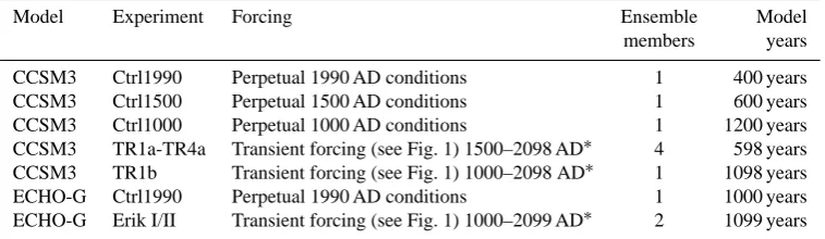
Table 1. Overview of simulations available for the analysis.
Model Experiment Forcing Ensemble Model
members years
CCSM3 Ctrl1990 Perpetual 1990 AD conditions 1 400 years
CCSM3 Ctrl1500 Perpetual 1500 AD conditions 1 600 years
CCSM3 Ctrl1000 Perpetual 1000 AD conditions 1 1200 years
CCSM3 TR1a-TR4a Transient forcing (see Fig. 1) 1500–2098 AD∗ 4 598 years CCSM3 TR1b Transient forcing (see Fig. 1) 1000–2098 AD∗ 1 1098 years
ECHO-G Ctrl1990 Perpetual 1990 AD conditions 1 1000 years
ECHO-G Erik I/II Transient forcing (see Fig. 1) 1000–2099 AD∗ 2 1099 years
∗Note that the transient simulations with CCSM3 and one simulation with ECHO-G use the A2 SRES scenarios for the future (see text
for details).
are used for the analysis. Note that the reanalysis product only relies on surface pressure measurements, so there is some concern about its ability to represent mid-tropospheric climate variability and climate variability in areas and time periods where surface data are scarcely available (e.g. the Arctic or the North Pacific in the early period of the reanal-ysis product). Still, Brönnimann et al. (2011) showed for example that TCR shows a rather close agreement to early upper air data, such as the geopotential height at 500 hPa. Moore et al. (2013) showed that TCR is able to realistically represent the surface climate variability in the North Atlantic region.
Besides the reanalysis product, the study is based on model results from two different fully coupled climate models. The first model is the Climate Community System Model, Ver-sion 3 (CCSM3) developed by NCAR (Collins et al., 2006), and consists of four components: atmosphere, ocean, land surface, and sea ice, all coupled without flux adjustments. To generate ensemble simulations the lowest resolution setting is selected. The atmospheric component has 26σ-pressure levels and a horizontal resolution of T31. The land surface shares the same horizontal resolution as the atmosphere. The ocean component has 25 unevenly spaced depth levels and a nominal horizontal resolution of 3◦(refined around Green-land and near the Equator to approximately 0.9◦). The ther-modynamic and dynamic sea ice component has the same horizontal resolution as the ocean component. To assess the role of the resolution, a horizontal resolution of T85 in the atmosphere and nominal 1◦ in the ocean is used for one simulation.
The second model (denoted as ECHO-G in the following) consists of four model components coupled, however, with an annual mean flux correction scheme for heat and freshwa-ter (Legutke and Voss, 1999) that averages out globally. The atmospheric component is the fourth version of the European Centre model of Hamburg (ECHAM4) with a horizontal res-olution of T30 and 19σ-pressure levels (Roeckner et al., 1996). The ocean component is the Hamburg ocean model in primitive equations (HOPE) with a horizontal resolution of 2.8◦×2.8◦ and 20 unevenly spaced vertical depth levels
(Wolff et al., 1997). Moreover, a land surface and a thermo-dynamic sea ice component are part of the model system.
Both models are used to perform (i) control simulations (Ctrl) with constant external forcing, and (ii) transient sim-ulations (TR1a-TR4a and TR1b with CCSM3; Erik I and II with ECHO-G) with time-varying external forcing as bound-ary conditions (Table 1). As control simulations, four sim-ulations with CCSM3 are available with perpetual 1000, 1500, and 1990 AD forcing. Details of the climatology and biases of the 1990 AD simulation in T31 can be found in Yeager et al. (2006). Additionally, a Ctrl simulation for 1990 AD conditions with a horizontal resolution of T85 is used to show the influence of the resolution on the re-sults.This simulation is provided by NCAR. The Ctrl1000 and Ctrl1500 simulations are discussed in Yoshimori et al. (2010) and Hofer et al. (2011). For ECHO-G, a Ctrl1900 sim-ulation is used. Its climatology is presented in Legutke and Voss (1999) and the variability of the Northern Hemisphere large-scale atmospheric circulation is investigated by Raible et al. (2001, 2004, 2005), Zorita et al. (2003), and Luksch et al. (2005).
Five transient simulations with CCSM3 are used, covering the last five centuries up to the last millennium. An ensem-ble of four simulations (TRa1 to TRa4) is integrated from 1500 to 2000 AD, where the initial states are obtained from different years of the Ctrl1500 simulation. One simulation (TRb1) spans the entire millennium, with an initial state from the Ctrl1000 simulation. For all five simulations, the same external forcing is applied, that is, greenhouse gas (GHG) concentrations, volcanic aerosols (in the stratosphere), and total solar irradiance (summarised in Fig. 1 – black lines). Further details of the simulations and the forcing functions are presented in Yoshimori et al. (2010), Hofer et al. (2011) and Lehner et al. (2012a, b). All simulations are extended to 2099 AD using the SRES A2 scenario (IPCC, 2001, 2007).
Fig. 1. Forcing from 1000 to 2100 AD for the CCSM3 (black) and
the ECHO-G (red) transient simulations: (a) solar and equivalent CO2forcing (including CO2, CH4, and N2O) with respect to mean
of the period 1500–1899, and (b) the forcing representing volcanic eruptions. The forcing in (a) is represented after conversion to the equivalent radiative forcing, assuming a planetary albedo of 0.31 and using the simplified formula given in IPCC (2001, Table 6.2). The inset in (a) focuses on the forcing functions from 1000 to 1850 AD. In (b) the optical depth in the visible band represents the volcanic forcing of the CCSM3 simulations, whereas in ECHO-G the volcanic forcing is just implemented by changes of the solar constant.
is based on older reconstructions for CH4and N2O and a
dif-ferent spline techniques is used for the same CO2data.
De-tails on these differences are discussed in Fernández-Donado et al. (2013). The volcanic forcing is only included as total solar irradiance changes; thus it only takes the direct short-wave effect of volcanic eruptions into account. As in the case of CCSM3 simulations, one simulation is extended to 2100 AD using the A2 SRES scenario. Details of these simu-lations are presented by González-Rouco et al. (2003, 2006, 2009) and Zorita et al. (2005). The simulations of both model setups are also compared with reconstructions and other sim-ulations of the last millennium by assessing the temperature response to the external forcing in Fernández-Donado et al. (2013). Note that the variability of the solar forcing used to drive the CCSM3 and ECHO-G simulations is rather large, that is, total solar irradiance changes between the Late Maun-der Minimum (1680–1715 AD) and the late 20th century are 0.23 % (CCSM3) and 0.29 % (ECHO-G), as presented in the multi-model comparison by Fernández-Donado et al. (2013).
3 Northern Hemisphere teleconnection patterns
In this section teleconnection patterns of the Northern Hemi-sphere are investigated. Therefore, we first compare the long-term mean behaviour of the model simulations with observa-tions, wherewith the classical teleconnection patterns are in-troduced and model biases in the correlation patterns are dis-cussed. The teleconnections are analysed by teleconnectivity
maps based on 500 hPa geopotential height (hereafter Z500) for winter months December to February (DJF), as first in-troduced by Wallace and Gutzler (1981). The teleconnectiv-ity is a field of anti-correlation based on the geopotential height in 500 hPa. Correlating one grid point with all oth-ers, the strongest negative correlation is searched for and denoted at this grid point. Assessing all grid points by this procedure leads to a field of negative correlation where the areas of stronger negative correlation correspond to centres of action of teleconnection patterns. These centres of action are combined by teleconnection axes (Wallace and Gutzler, 1981; Raible et al., 2006). These axes are identified using a one-point correlation technique, in other words, correlating a centre of action with the Z500 field and searching for the point which delivered the strongest negative correlation. The method is applied to monthly DJF data. Prior to the appli-cation of the teleconnectivity method the seasonal cycle is removed and the data is detrended. In the second part of this section the time-varying behaviour of the correlation patterns is presented.
3.1 Long-term mean
Applying the method of Wallace and Gutzler (1981) to the Z500 fields of the TCR data shows the well-known telecon-nection patterns for the current observational period from 1971–2000 AD (Fig. 2a). Teleconnectivity regions corre-sponding to the North Atlantic Oscillation (NAO) pattern, the West Pacific (WP) pattern, the Pacific North America (PNA) pattern, an area over Siberia and one connecting the east-ern Mediterranean with central Europe are identified. The latter shows weaker anti-correlations than for the aforemen-tioned regions. The teleconnections based on the entire pe-riod from 1871 to 2008 AD show a slight reduction of the anti-correlations (Fig. 2b). This reduction is particularly ob-served in the North Atlantic. More importantly, the telecon-nection patterns change in such a way that the more eastern position of the centres of action of the NAO during the pe-riod 1971–2000 AD (Fig. 2a) is shifted to the central Atlantic (Fig. 2b).
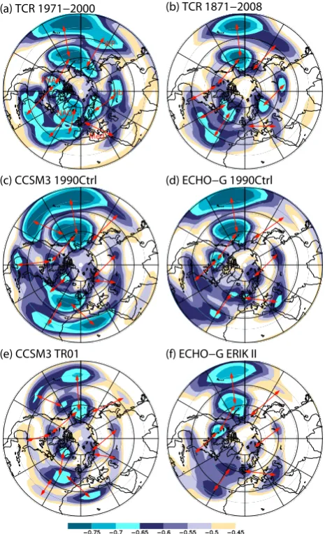
(a) TCR 1971−2000 (b) TCR 1871−2008
(c) CCSM3 1990Ctrl (d) ECHO−G 1990Ctrl
(e) CCSM3 TR01 (f) ECHO−G ERIK II PNA
NAO
Med Sib WP
Fig. 2. Teleconnectivity based on the 500 hPa geopotential height: (a) TCR for the reference period 1971–2000, (b) TCR for the
pe-riod 1871–2008, (c) Ctrl1990 of CCSM3, (d) Ctrl1990 of ECHO-G,
(e) TR1a, and (f) Erik II. Note that other simulations TR2a–TR4a
and TR1b show a similar pattern as (e) and Erik I resembles the pattern of (f), therefore they are not shown. The arrows illustrate teleconnection axes and are estimated by one-point correlations in each of the centres of action, as suggested by Wallace and Gutzler (1981) and Raible et al. (2006). They show NAO-type, PNA-type, and WP-type patterns as well as a pattern over Siberia (Sib) and a pattern connecting the eastern Mediterranean with central Europe (Med) as denoted in (a).
(Fig. 2c, d) over the Pacific and Siberia. The WP and the PNA patterns are nicely represented in all Ctrl experiments with some minor deviations in CCSM3, which simulates a north– south dipole structure in the eastern part of the Pacific and a slight westward shift of the Florida centre of the PNA pat-tern. The ECHO-G Ctrl experiment slightly underestimates the anti-correlation of the WP pattern.
The transient experiments of each model configuration re-semble the biases of the Ctrl experiments, and their strengths of anti-correlation generally become much weaker. Thus, the model simulations exhibit in some areas substantial biases in the correlation patterns and may only be partly able to cor-rectly simulate teleconnection patterns.
3.2 Time behaviour of teleconnection patterns
Differences in teleconnectivity between the entire TCR and the period from 1971–2000 AD already hint at a potential change in the strength and spatial pattern of correlations structures. To investigate the time dependence of the tele-connection patterns on decadal to multi-decadal timescales, the teleconnectivity based on Z500 is deduced using a 30-year running window. The agreement or disagreement with the current observed patterns is measured by pattern corre-lation between the patterns of the reference period (1971– 2000 AD) and patterns based on the running 30-year win-dow. The pattern correlation index is derived for two ar-eas: the North Atlantic European region (100◦W–50◦E, 0– 90◦N) and the North Pacific America region (230◦W–70◦W, 0–90◦N). A pattern correlation index ofr= 1 means that the teleconnection map of, e.g. a past 30-year period, perfectly matches with the current reference teleconnection map. The pattern correlation is a very demanding measure, as tests in the model world and the reanalysis show. Shifting a telecon-nection pattern by, e.g. two grid points, will cause the cor-relation pattern to deteriorate fromr= 1 to roughlyr= 0.85. Moreover, one could test whether a pattern correlation is sig-nificant or not. In doing so we find that the pattern correlation is statistically significant at the 1 % level when the correlation coefficientris greater than 0.53 for the Atlantic andr >0.65 for the Pacific (note that the difference is due to the high au-tocorrelation which deteriorates the degrees of freedom to roughly 19 for the Atlantic and 12 for the Pacific). Thus, we consider the resulting time series of pattern correlation to give evidence of periods of agreement with the current state for significant positive pattern correlation or disagree-ment for low or even negative pattern correlation, but we do not expect to reachr= 1.
1000 1100 1200 1300 1400 1500 1600 1700 1800 1900 2000 2100 Time [yr] -0.2 0 0.2 0.4 0.6 0.8 1 R Erik I Erik II
0 100 200 300 400 500 600 700 800 900 1000 1100 Model years -0.2 0 0.2 0.4 0.6 0.8 1 R Ctrl 1990 Ctrl 1500 Ctrl 1000 Ctrl 1990 T85
1000 1100 1200 1300 1400 1500 1600 1700 1800 1900 2000 2100 Time [yr] -0.2 0 0.2 0.4 0.6 0.8 1 R
0 100 200 300 400 500 600 700 800 900 1000 1100 Model years -0.2 0 0.2 0.4 0.6 0.8 1 R Ctrl 1990
1000 1100 1200 1300 1400 1500 1600 1700 1800 1900 2000 2100 Time [yr] -0.2 0 0.2 0.4 0.6 0.8 1 R TR1a TR2a TR3a TR4a TR1b (d) CCSM3 (e) ECHO−G (a) TCR (b) CCSM3 (c) ECHO−G
Corr. of ind. members Corr. of ensemble mean Ensemble mean of corr.
-0.75 -0.7 -0.65 -0.6 -0.55 -0.5 -0.45
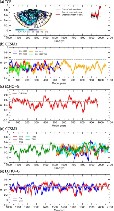
Fig. 3. Running spatial correlation time series using a 30-year
win-dow and the reference teleconnectivity pattern (inset in a) for the Atlantic: (a) TCR 1871 to 2010, (b) CCSM3 Ctrl simulations,
(c) Ctrl1990 of ECHO-G, (d) transient simulations with CCSM3,
and (e) transient simulations with ECHO-G. In (a) the black time se-ries shows the running spatial correlations using the ensemble mean TCR data; the grey time series are the running spatial correlations for each individual member of TCR and in red the mean of the grey time series is presented. The 1 % significance level of the pattern correlation is illustrated by the grey dashed line.
Moreover, the mean over all the ensemble members is similar to the correlation time series derived from the ensemble mean field which illustrates that TCR is rather well constrained in the North Atlantic.
The climate model simulations show a different picture (Fig. 3b–e). Overall the pattern correlation is reduced, which
1000 1100 1200 1300 1400 1500 1600 1700 1800 1900 2000 2100 Time [yr] 0 0.2 0.4 0.6 0.8 1 R
Corr. of ind. members Corr. of ensemble mean Ensemble mean of corr.
1000 1100 1200 1300 1400 1500 1600 1700 1800 1900 2000 2100
Time [yr] 0 0.2 0.4 0.6 0.8 1 R TR1a TR2a TR3a TR4a TR1b
1000 1100 1200 1300 1400 1500 1600 1700 1800 1900 2000 2100
Time [yr] 0 0.2 0.4 0.6 0.8 1 R Erik I Erik II
0 100 200 300 400 500 600 700 800 900 1000 1100
Model years 0 0.2 0.4 0.6 0.8 1 R Ctrl 1990 Ctrl 1500 Ctrl 1000 Ctrl 1990 T85
0 100 200 300 400 500 600 700 800 900 1000 1100
Model years 0 0.2 0.4 0.6 0.8 1 R Ctrl 1990 (b) CCSM3 (c) ECHO−G (d) CCSM3 (e) ECHO−G (a) TCR
-0.75 -0.7 -0.65 -0.6 -0.55 -0.5 -0.45
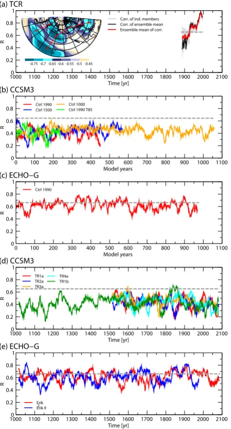
Fig. 4. As Fig. 3, but for the Pacific (see inset in a).
series of the Pacific behave similarly in the Ctrl and transient simulations and no external forcing imprint (or under future GHG forcing) is found.
Thus, we conclude that the temporal variability of simu-lated teleconnections of the Northern Hemisphere north of 20◦N is not different from internal climate variability for the
last 1000 years. Moreover, the results are not sensitive to the window size (not shown).
3.3 Spatial differences of teleconnection patterns
Further insights in the differences of the correlation patterns are gained by a composite analysis of the 30-year running window teleconnectivity patterns. Therefore, the time series
of pattern correlation are used as an index. If this index exceeds two standard deviations, the corresponding telecon-nectivity maps are selected and averaged in order to ob-tain the mean teleconnectivity map, which shows the closest agreement with the 1971–2000 baseline. If the index is be-low two standard deviations, the mean teleconnectivity map illustrates the pattern, which disagrees with the reference pat-tern of 1971–2000. These composites illustrate the charac-teristic teleconnection patterns of agreement and disagree-ment with the reference pattern. It shall be disagree-mentioned that the mean of different teleconnectivity patterns is not necessar-ily meaningful. However, in the analysis presented below the composite spans a similar range of correlation coefficients from−0.75 to−0.45 as the teleconnectivity deduced from a single 30-year period, e.g. 1971–2000. This indicates that the patterns included in the composites are very similar to each other. Therefore the application of a composite anal-ysis is trustworthy. As increasing the resolution of CCSM3 shows no difference, the T85 simulation is excluded from this analysis.
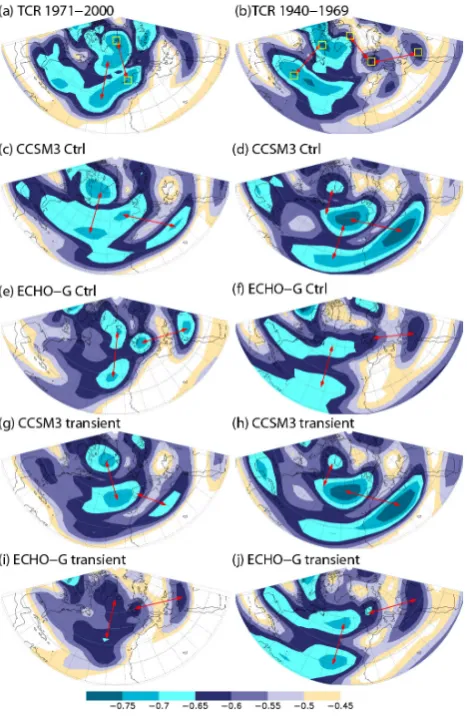
Fig. 5. Composites of teleconnectivity for all periods with high (left
panels) and low (right panels) spatial correlation in the Atlantic:
(a) TCR for period 1971–2000, (b) TCR for period 1940–1969, (c, d) composites of all CCSM3 Ctrl simulations, (e, f) composites of
the ECHO-G Ctrl1990 simulation, (g, h) composites of all CCSM3 transient simulations and (i, j) composites of all ECHO-G transient simulations. Note that the composites are selected according to a distance of at least two standard deviations from the mean of the corresponding spatial correlation times series of Fig. 3. The yellow squares in (a) and (b) show the location for the index definition in Sect. 4.
NAO-type pattern is shifted southwards by roughly 10◦, re-flecting the biases of ECHO-G (Sect. 3.1).
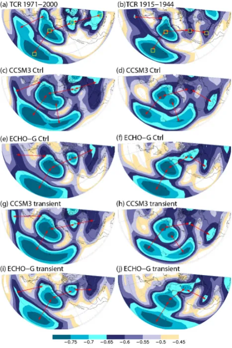
The North Pacific composite of the high pattern correlation index resembles the observed reference pattern from 1971– 2000 AD (Fig. 6, left column). The WP and PNA patterns are found in all simulations with only minor deviations in the locations of the centres of action (i.e. the composite of CCSM3 shows a tendency to split the tropical centre of the PNA pattern into two; Fig. 6c). Again, this is expected, as the pattern correlation indices are on average higher than for the Atlantic (Figs. 3 and 4). The observed anomalous period is from 1915 to 1944 AD, where the lowest pattern correlation
is found for the reliable period 1915–2008 (Fig. 4a). The cor-responding teleconnectivity (Fig. 6b) exhibits a change in the PNA pattern, shifting its centres of action over southwest Canada and over Florida to the Gulf of Mexico. Moreover, the WP pattern is shifted to the northwest. Concerning the model simulations for the anomalous patterns, we find that the PNA pattern is only weakly affected with a slight shift of the Florida centre of action. The main difference is found in the western part of the Pacific where the model simula-tions lose the WP pattern. Additionally, CCSM3 simulates a split of the tropical centre of the PNA, which is potentially a model bias (Sect. 3.1). As for the Atlantic, the Pacific com-posites of the model simulations show a similar range of tele-connectivity as the observations, therefore giving evidence of the robustness of these patterns. Overall, the changes in the North Pacific are less pronounced than in the Atlantic, favouring the conclusion that teleconnections in the Pacific are more stable than in the Atlantic.
4 Implications for proxy reconstructions
Proxy-based reconstructions for past atmospheric circulation patterns rely, as mentioned before, on the assumption of sta-tionarity in the relationship between a proxy signal and the corresponding atmospheric circulation. It has been illustrated in a number of studies that this assumption, primarily de-rived from late TCR, might not hold if one considers longer timescales (e.g. Lehner et al., 2012b). Moreover, within the observational period as well as in model simulations, the tele-connection patterns in both the Atlantic and Pacific change over time (as demonstrated in Sect. 3). This means that what are currently (1971–2000 AD) considered the dominant tele-connection patterns (e.g. NAO and PNA) do not necessar-ily look the same during other time periods of equal length. Therefore one can expect that, along with changes in the tele-connection patterns, the correlation strength of a fixed proxy site with the atmospheric circulation may change.
The period of maximum disagreement with the refer-ence teleconnectivity pattern in the Atlantic in TCR (1940– 1969 AD) features the NAO-like dipole, but substantially shifted to the west (Fig. 5b). This pattern is termed the Baffin Island–West Atlantic (BWA) pattern (Shabbar et al., 1997) and is defined here from the maxima of teleconnectivity in the North Atlantic during this time period:
BWA=0.5· [Z0(39◦N; 62◦W)−Z0(68◦N; 64◦W)], (1) withZ0being the normalised Z500 time series. The degree of independence of the BWA from the NAO has been discussed (e.g. Shabbar et al., 1997) and new studies describe a distinct anti-phasing of BWA and NAO during certain periods of the twentieth century (e.g. Moore et al., 2011)
Fig. 6. Composites of teleconnectivity for all periods with high
(left panels) and low (right panels) spatial correlation in the Pacific:
(a) TCR for period 1971–2000, (b) TCR for period 1915–1944, (c, d) composites of all CCSM3 Ctrl simulations, (e, f) composites of
the ECHO-G Ctrl1990 simulation, (g, h) composites of all CCSM3 transient simulations and (i, j) composites of all ECHO-G transient simulations. Note that the composites are selected according to a distance of at least two standard deviations from the mean of the corresponding spatial correlation times series of Fig. 4. The yellow squares in (a) and (b) show the location for the index definition in Sect. 4.
AWAVE=0.5·Z0(50◦N; 7◦E)−0.25· [Z0(32◦N;
37◦E)+Z0(80◦N; 29◦W)]. (2) AWAVE bears similarities with the North Sea–Caspian Pat-tern (NCP; Kutiel and Benaroch, 2002), however, it features a third node at higher latitudes and has the eastern node shifted south compared to NCP.
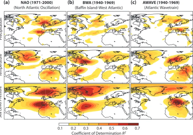
The usefulness of these two indices, BWA and AWAVE, in describing climate variability over time can now be tested and compared against the NAO. Figure 7 shows the coef-ficient of determination R2 (the squared correlation of an index with a climate field, serving as an estimate of ex-plained variance) of the indices NAO, BWA, and AWAVE
for the classical proxy variables of precipitation and sur-face air temperature (SAT) during the phase of strong and weak NAO-like teleconnection (1971–2000 and 1940–1969, respectively). Additionally,R2 is also shown for sea level pressure (SLP). As known from earlier studies (e.g. Hurrell, 1995), the NAO describes variability of precipitation in the western Mediterranean region and northern Europe, SAT in central Europe and Greenland, and the SLP dipole between Iceland and the Azores. Compared to the NAO, the BWA shows smaller coefficients for precipitation, but larger coeffi-cients for SAT in the western part of the North Atlantic. Simi-lar to the NAO it has an equivalent barotropic signature in the SLP. The AWAVE explains a substantial amount of precipita-tion and SAT variability mainly over Europe. It is interesting to see that the AWAVE has no equivalent barotropic imprint in SLP, but features a SLP dipole with a southern node cen-tred on Europe.
By averaging R2 across the North Atlantic domain and – more important for proxies – the continental Atlantic do-main, the time evolution of the coefficient of determination is illustrated (Fig. 8). The NAO describes North Atlantic-wide climate variability best during roughly the last 30– 40 years, when it profits from high values in selected areas, expressed as a large area fraction of values exceeding 0.4 (0.4 = 40 % variability explained, which is a good estimate for mode dominance). Before that, the spatially averagedR2 of NAO drops and BWA or AWAVE usually show higher in-dex values.
This becomes even more apparent when considering only the land area, where the AWAVE describes a larger fraction of the climate variability than the NAO for most of the time. Except for the period around 1920, when none of the indices shows particularly high values, the AWAVE displays higher or equally high values as the NAO in both spatial average and area fraction>0.4 ofR2. The BWA index shows good spatially averaged coefficients, but covers only a small area with values>0.4.
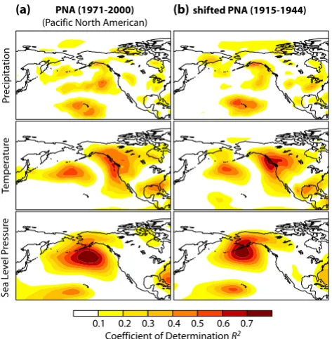
As mentioned in the previous section, changes are much weaker for the PNA. The PNA during 1971–2000 and its shifted expression during the period of largest disagreement, 1915–1944, are defined as
PNA=0.25· [Z(17◦N,173◦W)−Z(46◦N, 165◦W)
+Z(58◦N,105◦W)−Z(28◦N,83◦W)] (3)
and
PNAshifted =0.25·
Z(19◦N,173◦W)−Z(53◦N,169◦W)
+Z(45◦N,113◦W)−Z(30◦N, 98◦W)
NAO (1971-2000) (North Atlantic Oscillation)
BWA (1940-1969) (Baffin Island-West Atlantic)
AWAVE (1940-1969) (Atlantic Wavetrain)
0.1 0.2 0.3 0.4 0.5 0.6 0.7 Coefficient of Determination R2
Temp
er
atur
e
Pr
ecipita
tion
Sea L
ev
el P
ressur
e
(a) (b) (c)
Fig. 7. Coefficient of determination of (a) the North Atlantic Oscillation (NAO), (b) the Baffin Island–West Atlantic pattern (BWA), and (c) the Atlantic Wave Train (AWAVE) for precipitation, surface air temperature, and sea level pressure, deduced from the TCR ensemble
mean. The time period 1971–2000 is defined as the reference period; 1940–1969 is the 30-year period of largest disagreement in teleconnec-tivity from the reference period. See text for further details.
Fig. 8. Explanatory power of teleconnection modes in TCR. (a; upper lines, leftyaxis) 30-year moving spatially averaged coefficient of determinationR2of the NAO, BWA, and AWAVE for precipitation over the North Atlantic domain (see text and Fig. 7 for details on domain and indices). (a; lower lines, rightyaxis) 30-year moving average of fraction of domain area whereR2>0.4. Vertical lines mark the two periods shown in Fig. 7. (b) Same as (a) but for temperature. (c, d) Same as (a, b) but for the North Atlantic land only. Shown is the range of the ensemble members and the ensemble mean of the individual members.
5 Conclusions
Changing correlation structures of the Northern Hemi-sphere atmospheric circulation are investigated for the pe-riod 1000–2100 AD using reanalysis data and different sets
PNA (1971-2000) (Pacific North American)
shifted PNA (1915-1944)
0.1 0.2 0.3 0.4 0.5 0.6 0.7 Coefficient of Determination R2
Temp
er
atur
e
Pr
ecipita
tion
Sea L
ev
el P
ressur
e
(a) (b)
Fig. 9. As Fig. 7 but for (a) the Pacific North American pattern
(PNA) and (b) the shifted PNA.
showing a splitting in a north–south dipole in the western part of the North Atlantic, and a wave train pattern in the east-ern part and over Europe during some periods. The observed structural changes in the North Pacific and over North Amer-ica are smaller compared to the North Atlantic. The findings for the North Atlantic are in line with earlier studies assum-ing a non-stationarity of the centres of action of the NAO (Raible et al., 2001, 2006), a continuum of teleconnection patterns (Franzke and Feldstein, 2005) and recently a postu-lated changing linear combination of the leading modes of variability in the North Atlantic (Moore et al., 2013).
Expanding the analysis further back in time and into the future with model simulations complements the picture, al-though model biases are evident in simulating the telecon-nection patterns and the locations of their centres of ac-tion. These biases remain even when the resolution is in-creased, as illustrated by one model set up. This is a hint that climate models still suffer from under-representation of important atmospheric processes, such as blocking ac-tion (Woollings et al., 2010a; Buehler et al., 2011) or stratosphere–troposphere interaction (e.g. Kodera et al., 1996) and demonstrate our incomplete understanding of at-mosphere dynamics. Despite these biases, the model simu-lations show strong variability of the teleconnection patterns over time, and to some extent similar deviations are found in the reanalysis data for the past 130 years. Comparing the transient simulations with external forcing and with the be-haviour of the corresponding control simulations shows that the temporal variability of teleconnections of the Northern Hemisphere north of 20◦N is, over time, not different from
internal climate variability for the last 1000 years. Even for the rather high external forcing of the A2 scenario for the fu-ture, a systematic change is not found. This contradicts ear-lier findings by Ulbrich and Christoph (1999) who suggested a north-eastwards shift of the NAO centres of action under greenhouse-gas-induced warming. Whether this is a robust finding is questionable, as our ensemble of opportunity en-compasses only three simulations and should be assessed in a wider pool of simulations such as CMIP5 (Taylor et al., 2012).
The reasons for changing teleconnection structures are less understood. The periods in the reanalysis where teleconnec-tion patterns disagree with the current locateleconnec-tions resemble, to some extent, periods with different atmosphere–ocean cou-pling. Raible et al. (2001) identified periods during which decadal-scale variability of the NAO coincides with strong coupling of the atmosphere to the ocean underneath, whereas periods dominated by interannual variability seem to be re-lated to tropical SST changes in the Pacific. In line with these changes, the coupling between the Atlantic and Pa-cific is found to be variable over time (Raible et al., 2004; Luksch et al., 2005; Pinto et al., 2011). Other reasons such as stratosphere–troposphere interaction (Kodera et al., 1996; Woollings et al., 2010a) or sea–ice interaction with the at-mosphere (e.g. Lehner et al., 2013) are also potential drivers of such changes, but this needs to be the focus of future research.
Another important conclusion concerns the reconstruction of modes of variability back in time. Such reconstructions rely on a stationary relationship between the proxy site and the atmospheric mode, often implying that the dominant at-mospheric mode does not change over time. We show that changes in the dominant mode occur already in the twenti-eth century, in particular in the North Atlantic. The explana-tory power of the NAO for climate variability, for example, is highest in the last 30–40 years. Before that, the emergence of other modes draws a more complex picture of atmospheric variability and contrasts with the simplified interpretation of atmospheric teleconnections usually presented in paleocli-mate reconstructions.
Selected proxy sites may be used to reconstruct a known atmospheric mode (e.g. the NAO as we know it from 1971– 2000), but we have no good means yet to determine whether this was actually the dominant mode. However, knowing the dominant mode is important for the interpretation of inde-pendent proxies, as different modes can imply different phys-ical mechanisms for a recorded proxy signal. Given the pop-ularity in the literature to relate new proxies to the dominant modes (e.g. Trouet et al., 2009; Olsen et al., 2012), it is im-portant to develop gridded reconstructions of sea level pres-sure (Küttel et al., 2010) along with new methods that allow us to determine the dominant mode from a proxy network.
Further, they advise future reconstructions of atmospheric modes to thoroughly test and carefully select the proxies to be used and, most importantly, to cautiously interpret their results with respect to what part of past climate variability can be explained by a specific reconstruction.
Acknowledgements. This work is supported by the Siner-gia project FUPSOL funded by the Swiss National Science Foundation. 20th Century Reanalysis data is provided by the NOAA/OAR/ESRL PSD, Boulder, Colorado, USA (from their website at http://www.esrl.noaa.gov/psd/). The CCSM3 simulations are performed on the super computing architecture of the Swiss National Supercomputing Centre (CSCS). LFD and JFGR were supported by CGL 2011-29677-602-02, CGL 2011-29672-602-01, and the FPU grant AP2009-4061.
Edited by: H. Goosse
References
Barnston, A. G. and Livezey, R. E.: Classification, seasonality and persistence of low-frequency atmospheric circulation patterns, Mon. Weather Rev., 115, 1825–1850, 1987.
Brönnimann, S., Compo, G. P., Spadin, R., Allan, R., and Adam, W.: Early ship-based upper-air data and comparison with the Twenti-eth Century Reanalysis, Clim. Past, 7, 265–276, doi:10.5194/cp-7-265-2011, 2011.
Buehler, T., Raible, C. C., and Stocker, T. F.: On the relation of extreme North Atlantic blocking frequencies, cold spells, and droughts in ERA-40 in winter, Tellus, 63, 212–222, 2011. Casty, C., Raible, C. C., Stocker, T. F., Wanner, H., and Luterbacher,
J.: European climate pattern variability since 1766, Clim. Dy-nam., 29, 791–805, 2007.
Collins, W. D., Bitz, C. M., Blackmon, M. L., Bonan, G. B., Bretherton, C. S., Carton, J. A., Chang, P., Doney, S. C., Hack, J. J., Henderson, T. B., Kiehl, J. T., Large, W. G., McKenna, D. S., Santer, B. D., and Smith, R. D.: The Community Climate System Model version 3 (CCSM3), J. Climate, 19, 2122–2143, 2006.
Compo, G., Whitaker, J., and Sardeshmukh, P.: Feasibility of a 100-year reanalysis using only surface pressure data, B. Am. Meteo-rol. Soc., 87, 175–190, 2006.
Compo, G. P., Whitaker, J. S., Sardeshmukh, P. D., Matsui, N., Al-lan, R. J., Yin, X., Gleason Jr., B. E., Vose, R. S., Rutledge, G., Bessemoulin, P., Broennimann, S., Brunet, M., Crouthamel, R. I., Grant, A. N., Groisman, P. Y., Jones, P. D., Kruk, M. C., Kruger, A. C., Marshall, G. J., Maugeri, M., Mok, H. Y., Nordli, O., Ross, T. F., Trigo, R. M., Wang, X. L., Woodruff, S. D., and Worley, S. J.: The Twentieth Century Reanalysis Project, Q. J. Roy. Me-teorol. Soc., 137, 1–28, 2011.
Cook, E. R., D’Arrigo, R. D., and Mann, M. E.: A well-verified, multiproxy reconstruction of the winter North Atlantic Oscilla-tion index since AD 1400, J. Climate, 15, 1754–1764, 2002. Defant, A.: Die Schwankungen der atmosphärischen Zirkulation
über dem nordatlantischen Ozean im 25-jährigen Zeitraum 1881–1905, Geogr. Ann., 6, 13–41, 1924.
Fernández-Donado, L., González-Rouco, J. F., Raible, C. C., Am-mann, C. M., Barriopedro, D., García-Bustamante, E., Jungclaus, J. H., Lorenz, S. J., Luterbacher, J., Phipps, S. J., Servonnat, J., Swingedouw, D., Tett, S. F. B., Wagner, S., Yiou, P., and Zorita, E.: Large-scale temperature response to external forcing in simu-lations and reconstructions of the last millennium, Clim. Past, 9, 393–421, doi:10.5194/cp-9-393-2013, 2013.
Franzke, C. and Feldstein, S. B.: The continuum and dynamics of Northern Hemisphere teleconnection patterns, J. Atmos. Sci., 62, 3250–3267, 2005.
González-Rouco, F., von Storch, H., and Zorita, E.: Deep soil tem-perature as proxy for surface air-temtem-perature in a coupled model simulation of the last thousand years, Geophys. Res. Lett., 30, doi:10.1029/2003GL018264, 2003.
González-Rouco, J. F., Beltrami, H., Zorita, E., and von Storch, H.: Simulation and inversion of borehole temperature profiles in sur-rogate climates: Spatial distribution and surface coupling, Geo-phys. Res. Lett., 33, doi:10.1029/2005GL024693, 2006. González-Rouco, J. F., Beltrami, H., Zorita, E., and Stevens, M. B.:
Borehole climatology: a discussion based on contributions from climate modeling, Clim. Past, 5, 97–127, doi:10.5194/cp-5-97-2009, 2009.
Hann, J.: Zur Witterungsgeschichte von Nord-Grönland, Westküste, Meteorl. Z., 15, 787–799, 1890.
Hofer, D., Raible, C. C., and Stocker, T. F.: Variations of the At-lantic meridional overturning circulation in control and tran-sient simulations of the last millennium, Clim. Past, 7, 133–150, doi:10.5194/cp-7-133-2011, 2011.
Hurrell, J. W.: Decadal trends in the North Atlantic Oscillation: Re-gional temperatures and precipitation, Science, 269, 676–679, 1995.
Hurrell, J. W. and Deser, C.: North Atlantic climate variability: The role of the North Atlantic Oscillation, J. Mar. Syst., 78, 28–41, 2009.
Hurrell, J. W., Hoerling, M. P., Phillips, A., and Xu, T.: Twentieth century North Atlantic climate change, Part I: Assessing deter-minism, Clim. Dynam., 23, 371–389, 2004.
IPCC: Climate Change 2001: The Scientific Basis, Contribution of Working Group I to the Third Assessment Report of the Inter-governmental Panel on Climate Change, Cambridge University Press, Cambridge, UK and New York, NY, USA, 2001. IPCC: Climate Change 2007: The Physical Science Basis,
Contri-bution of Working Group I to the Forth Assessment Report of the Intergovernmental Panel on Climate Change, Cambridge Univer-sity Press, Cambridge, UK and New York, NY, USA, 2007. Kodera, K., Chiba, M., Koide, H., Kitoh, A., and Nikaidou, Y.:
In-terannual variability of the winter stratosphere and troposphere in the Northern Hemisphere, J. Meteorol. Soc. Jpn., 74, 365–382, 1996.
Kutiel, H. and Benaroch, Y.: North Sea-Caspian Pattern (NCP) – an upper level atmospheric teleconnection affecting the Eastern Mediterranean: Identification and definition, Theor. Appl. Clima-tol., 71, 17–28, 2002.
Legutke, S. and Voss, R.: The Hamburg Atmosphere-Ocean Cou-pled circulation model ECHO-G, Tech. Rep. 18, Deutsches Kli-marechenzentrum, Hamburg, Germany, 62 pp., 1999.
Lehner, F., Raible, C. C., Hofer, D., and Stocker, T. F.: The freshwa-ter balance of polar regions in transient simulations from 1500 to 2100 AD using a comprehensive coupled climate model, Clim. Dynam., 39, 347–363, 2012a.
Lehner, F., Raible, C. C., and Stocker, T. F.: Testing the robustness of a precipitation proxy-based North Atlantic Oscillation recon-struction, Quaternary Sci. Rev., 45, 85–94, 2012b.
Lehner, F., Born, A., Raible, C. C., and Stocker, T. F.: Amplified in-ception of European Little Ice Age by sea ice-ocean-atmosphere feedbacks, J. Climate, 26, 7586–7602, 2013.
Lorenz, E. N.: The nature and theory of the general circulation of the atmosphere, Tech. rep., WMO-No. 218, TP 115, WMO, Geneva, Switzerland, 161 pp., 1967.
Luksch, U., Raible, C. C., Blender, R., and Fraedrich, K.: Cyclone track and decadal Northern Hemispheric regimes, Meteorol. Z., 14, 747–753, 2005.
Luterbacher, J., Schmutz, C., Gyalistras, D., Xoplaki, E., and Wan-ner, H.: Reconstruction of monthly NAO and EU indices back to AD 1675, Geophys. Res. Lett., 26, 2745–2748, 1999.
Luterbacher, J., Xoplaki, E., Dietrich, D., Jones, P. D., Davies, T. D., Portis, D., Gonzalez-Rouco, J. F., von Storch, H., Gyalistras, D., Casty, C., and Wanner, H.: Extending North Atlantic Oscilla-tion reconstrucOscilla-tions back to 1500, Atmos. Sci. Lett., 2, 114–124, 2002.
Mann, M. E.: Large-scale climate variability and connections with the Middle East in past centuries, Climatic Change, 55, 287–314, 2002.
Moore, G. W. K., Holdsworth, G., and Alverson, K.: Climate change in the North Pacific region over the past three centuries, Nature, 420, 401–403, 2002.
Moore, G. W. K., Pickart, R. S., and Renfrew, I. A.: Complexi-ties in the climate of the subpolar North Atlantic: a case study from the winter of 2007, Q. J. Meteorol. Soc., 137, 757–767, doi:10.1002/qj.778, 2011.
Moore, G. W. K., Renfrew, I. A., and Pickart, R. S.: Multidecadal mobility of the North Atlantic Oscillation, J. Climate, 26, 2453– 2466, 2013.
Olsen, J., Anderson, N. J., and Knudsen, M. F.: Variability of the North Atlantic Oscillation over the past 5,200 years, Nat. Geosci., 5, 808–812, 2012.
Pinto, J. G. and Raible, C. C.: Past and recent changes in the NAO, Interdiscip. Rev. Clim. Change, 3, 79–90, 2012.
Pinto, J. G., Reyers, M., and Ulbrich, U.: The variable link between PNA and NAO in observations and in multi-century CGCM sim-ulations, Clim. Dynam., 36, 337–354, 2011.
Raible, C. C., Luksch, U., Fraedrich, K., and Voss, R.: North At-lantic decadal regimes in a coupled GCM simulation, Clim. Dy-nam., 18, 321–330, 2001.
Raible, C. C., Luksch, U., and Fraedrich, K.: Precipitation and Northern Hemisphere regimes, Atmos. Sci. Lett., 5, 43–55, 2004. Raible, C. C., Stocker, T. F., Yoshimori, M., Renold, M., Beyerle, U., Casty, C., and Luterbacher, J.: Northern Hemispheric trends of pressure indices and atmospheric circulation patterns in obser-vations, reconstructions, and coupled GCM simulations, J. Cli-mate, 18, 3968–3982, 2005.
Raible, C. C., Casty, C., Luterbacher, J., Pauling, A., Esper, J., Frank, D. C., Büntgens, U., Roesch, A. C., Wild, M., Tschuck, P., Vidale, P.-L., Schär, C., and Wanner, H.: Climate variability – observations, reconstructions and model simulations, Climatic Change, 79, 9–29, 2006.
Roeckner, E., Arpe, K., and Bengtsson, L.: The atmospheric Gen-eral Circulation Model ECHAM-4: Model description and sim-ulation of present-day climate, Tech. Rep. 218, Max-Planck-Institut, Hamburg, Germany, 90 pp., 1996.
Schmutz, C., Luterbacher, J., Gyalistras, D., Xoplaki, E., and Wan-ner, H.: Can we trust proxy-based NAO index reconstructions?, Geophys. Res. Lett., 27, 1135–1138, 2000.
Shabbar, A., Higuchi, K., Skinner, W., and Knox, J.: The association between the BWA index and winter surface temperature variabil-ity over eastern Canada and west Greenland, Int. J. Climatol., 17, 1195–1210, 1997.
Stephenson, D. B., Wanner, H., Broennimann, S., and Luterbacher, J.: The North Atlantic Oscillation, Climatic significance and en-vironmental impact, Geophys. Monogr. Ser., 134, 37–50, 2003. Taylor, K. E., Stouffer, R. J., and Meehl, G. A.: An overview of
CMIP5 and the experiment design, B. Am. Meteorol. Soc., 93, 485–498, 2012.
Trouet, V. and Taylor, A. H.: Multi-century variability in the Pacific North American circulation pattern reconstructed from tree rings, Clim. Dynam., 35, 953–963, 2010.
Trouet, V., Esper, J., Graham, N. E., Baker, A., Scourse, J. D., and Frank, D. C.: Persistent positive North Atlantic Oscillation mode dominated the Medieval Climate Anomaly, Science, 324, 78 – 80, 2009.
Ulbrich, U. and Christoph, M.: A shift of the NAO and increasing storm track activity over Europe due to anthropogenic Green-house gas forcing, Clim. Dynam., 15, 551–559, 1999.
Wallace, J. M. and Gutzler, D. S.: Teleconnections in the geopo-tential height field during the Northern Hemisphere winter, Mon. Weather Rev., 109, 782–812, 1981.
Wanner, H., Brönnimann, S., Casty, C., Gyalistras, D., Luterbacher, J., Schmutz, C., Stephenson, D. B., and Xoplaki, E.: North At-lantic Oscillation – concepts and studies, Surv. Geophys., 22, 321–382, 2001.
Wolff, J. O., Maier-Reimer, E., and Legutke, S.: The Ham-burg Ocean primitive equation model HOPE, Tech. Rep. 13, Deutsches Klimarechenzentrum, Hamburg, Germany, 1997. Woollings, T., Charlton-Perez, A., Ineson, S., Woollings,
T., Charlton-Perez, A., Ineson, S., Marshall, A. G., and Masato, G.: Associations between stratospheric variability and tropospheric blocking, J. Geophys. Res., 115, D06108, doi:10.1029/2009JD012742, 2010a.
Woollings, T. J., Hannachi, A., Hoskins, B., and Turner, B. A.: A regime view of the North Atlantic Oscillation and its response to anthropogenic forcing, J. Climate, 23, 1291–1307, 2010b. Yeager, S. G., Shields, C. A., Large, W. G., and Hack, J. J.: The
low-resolution CCSM3, J. Climate, 19, 2545–2566, 2006. Yoshimori, M., Raible, C. C., Stocker, T. F., and Renold, M.:
Zorita, E. and Gonzalez-Rouco, F.: Are temperature-sensitive prox-ies adequate for North Atlantic Oscillation reconstructions?, Geophys. Res. Lett., 29, 1703, doi:10.1029/2002GL015404, 2002.
Zorita, E., Gonzalez-Rouco, J. F., and Legutke, S.: Statistical tem-perature reconstruction in a 1000-year-long control climate simu-lation an excercise with Mann’s et al. (1998) method, J. Climate, 16, 1378–1390, 2003.