Analysis of stochastic model for nonlinear volcanic dynamics

Nonlin. Processes Geophys., 22, 197–204, 2015 www.nonlin-processes-geophys.net/22/197/2015/ doi:10.5194/npg-22-197-2015

© Author(s) 2015. CC Attribution 3.0 License.

Analysis of stochastic model for nonlinear volcanic dynamics

D. V. Alexandrov, I. A. Bashkirtseva, and L. B. Ryashko

Department of Mathematical Physics, Ural Federal University, Lenin ave. 51, 620000 Ekaterinburg, Russia Correspondence to: L. Ryashko (lev.ryashko@urfu.ru)

Received: 11 November 2014 – Published in Nonlin. Processes Geophys. Discuss.: 3 December 2014 Revised: 10 March 2015 – Accepted: 12 March 2015 – Published: 7 April 2015

Abstract. Motivated by important geophysical applications we consider a dynamic model of the magma-plug system previously derived by Iverson et al. (2006) under the influ-ence of stochastic forcing. Due to strong nonlinearity of the friction force for a solid plug along its margins, the initial de-terministic system exhibits impulsive oscillations. Two types of dynamic behavior of the system under the influence of the parametric stochastic forcing have been found: random tra-jectories are scattered on both sides of the deterministic cycle or grouped on its internal side only. It is shown that disper-sions are highly inhomogeneous along cycles in the presence of noises. The effects of noise-induced shifts, pressure sta-bilization and localization of random trajectories have been revealed by increasing the noise intensity. The plug velocity, pressure and displacement are highly dependent of noise in-tensity as well. These new stochastic phenomena are related to the nonlinear peculiarities of the deterministic phase por-trait. It is demonstrated that the repetitive stick–slip motions of the magma-plug system in the case of stochastic forcing can be connected with drumbeat earthquakes.

1 Introduction

It is well-known that the behavior of volcanic systems is enormously complex so that a lot of nonlinear feedbacks lead to multiple states even during a single eruption (Tanaka et al., 2014). Without better modeling forecasts of these dynamic processes, the highly important questions of where, when and how volcanic eruptions occur will remain substantially em-pirical. Nowadays, an elaboration of the adequate mathemat-ical models for volcanic dynamics is a challenging problem (Melnik and Sparks, 1999; Barmin et al., 2002; Nakanishi and Koyaguchi, 2008; Costa et al., 2012).

Many uncertainties in physical parameters of volcanic dy-namics (Woo, 2000) lead to a conclusion that like the cli-mate systems (see, among others, Saltzman, 2002; Alexan-drov et al., 2014), volcanoes, representing stochastic and chaotic systems, need to be described in terms of proba-bilities (Sparks, 2003; Bebbington and Marzocchi, 2011). Stochastic approaches and mathematical formalisms can be found in Gardiner (2009).

It is well-known, that an interplay between nonlinear-ity and noise can generate various probabilistic phenom-ena such as noise-induced transitions (Horsthemke and Lefever, 1984), stochastic resonance (McDonnell et al., 2008; Pikovsky and Kurths, 1997; Arathi, 2013), and noise-induced chaos (Lai and Tél, 2011; Bashkirtseva et al., 2012). Stochastic effects in nonlinear models are the subjects of intensive investigations in various research domains (Hors-themke and Lefever, 1984; Lindner et al., 2004; Bashkirtseva et al., 2013; Alexandrov et al., 2013).

198 D. Alexandrov et al.: Stochastic volcanic model

Figure 1. A scheme of the plug dynamics.

model to demonstrate unusual dynamic behavior of similar volcanic systems under the influence of parametric noises.

In order to explain interactions between solid-state extru-sion and persistent drumbeat earthquakes at MSH, Iverson et al. (2006) developed a model based on recurrent stick–slip motions of the solid plug along its margins with the friction forceF (Fig. 1). Let us briefly discuss the main principles of this dynamic model. The magma influx comes to the base of an eruptive conduit from below with a nearly steady rate Q. A solid dacite plug of solidified magma blocks the con-duit from above so that its lower boundary is mobile due to the effects of pressure and basal accretion with mass rateρB from below (ρ andB stand for the magma bulk density and the volumetric rate of magma crystallization). The total plug mass mchanges with time because the difference in mass ratesρB andρrEas m=m0+κt (hereρris the plug bulk density,Eis the volumetric rate of surface erosion,m0is the initial plug mass, t is the process time, and κ=ρB−ρrE is assumed constant). The horizontal cross-sectional areaA, the magma compressibilityα1and the conduit wall compli-anceα2are estimated by Iverson et al. (2006). The dynamic process of plug extrusion is controlled by the plug weightmg and the friction forceF dependent of the plug velocityu(g is the acceleration due to gravity) whereas the conduit vol-umeV is governed by the law of mass conservation. A three-parametric differential model connecting independent vari-ablesu,pandV (pis the pressure) was derived by Iverson et al. (2006). Below we use this model to demonstrate some new special aspects of nonlinear dynamics of volcanic sys-tems under the influence of stochastic noises.

(a)

0 5 10

x 10−4 1.2934

1.2935 1.2936

x 107

p

u

C

(b)

0 10

x 10−5 1.2935

x 107

p

u

C

Figure 2. (a)

Projection of the phase portrait of the deterministic system,

p

(Pa) vs.

u

(

m s

).

(b)

illustrates an

enlargement near unstable equilibrium (open circle). The dashed red line is a pseudo-separatrix. Physical

pa-rameters of the system under consideration are (Iverson et al., 2006):

B

=

Q

= 2 m

s

,

m

0

=

3.6

×

10

kg,

A

=

30 000

m

,

p

=

12 936

×

10

Pa

,

α

= 10

Pa

,

α

= 10

Pa

,

F

=

3528

×

10

kg m s

,

u

=

0.1Q/A

=

66 667

×

10

m s

,

V

=

6.32

×

10

m

,

c

=

1.7

×

10

,

g

= 9.8 m s

,

ρ

=

ρ

= 2000 kg m

,

κ

= 0

.

10

Figure 2. (a) projection of the phase portrait of the

determinis-tic system, p (Pa) vs. u (m s−1). (b) illustrates an enlargement near unstable equilibrium (open circle). The dashed red line is a pseudo-separatrix. Physical parameters of the system under con-sideration are (Iverson et al., 2006)B=Q=2 m3s−1,m0=3.6×

1010kg,A=30 000 m2,p0=12 936×103Pa,α1=10−7Pa−1,

α2=10−9Pa−1,F0= 3528×107 kg m s−2,uref=0.1Q/A=

6.67×10−6m s−1,V0=6.32×105m3,c=1.7×10−4,g=9.8

m s−2,ρ0=ρr=2000 kg m−3, andκ=0.

2 The model and its deterministic behavior

The following system of reduced governing equations based on the laws of conservation of the solid plug linear momen-tum, solid plug mass and conduit fluid mass was derived and discussed in detail by Iverson et al. (2006). These equations can be written in the form of

du

dt = −g+ 1 m0+κt

(pA−κu−F ), (1)

dp dt = −

1 (α1+α2)V

(Au+RB−Q), (2)

dV dt =

α1 α1+α2

(Au+RB−Q)+Q−B, (3)

D. Alexandrov et al.: Stochastic volcanic model 199

0 100 200 300 400 0

5 10 15

x 10−4

u

t

1.2934 1.2935

x 107

t

p

0 100 200 300 400 6.32

6.321 x 105

t

V

Figure 3.Time series of the cycle shown in Fig. 2:u(m s−1_{),p(Pa) ansV (m}3_{) as functions of timet(s).}

(a)

0 10

x 10−4 1.2934

1.2935 1.2936

x 107

u

p

(b)

0 100 200 300 400 0

5 10 15

x 10−4

t

u

Figure 4. (a)illustrates a projection of the phase portraitp(Pa) vs.u(m s−1_{) of the deterministic system.(b)}

showsu(m s−1_{) as a function oft(s). These dependencies are plotted for different valuesV}

0:V0= 105m3

(blue),V0= 6.32×105m3(red), andV0= 106m3(green).

11

Figure 3. Time series of the cycle shown in Fig. 2:u(m s−1),p(Pa) andV (m3) as functions of timet(s).

by a function (Iverson et al., 2006):

F (u)=sgn(u)f₀(u), f₀(u)=F₀1−csinh−1|u/u_ref|

, (4) where sgn(u)is the sign ofu,F0is the friction force at static equilibrium,c1 is a rate-weakening parameter andurefis a reference value of u (Iverson et al., 2006). Equation (4) includes the main physical aspects of the process: the fric-tion force atu=0 abruptly changes its sign due to the fact that the gravity force, which shifts the plug in downward di-rection, is opposite to the friction force. However, an abrupt behavior of Eq. (4) is not a good physical approximation of the friction force. Therefore, let us model this force by the close continuous function:

F (u)=sgn(u)f1(u), (5)

where

f1(u)=

(

f0(u), |u| ≥uref

F0|_uu

ref|, 0<|u|< uref .

In present paper we focus on the autonomous case, when κ=0. The model (Eqs. 1–3) demonstrates the stick– slip oscillations (see Figs. 2 and 3). An important point is that this system has only one unstable equilibrium (u, p, V )for anyV0, whereu =

Q

A =

2 3×10

−4_{m s}−1_,p= p0=12 936×103Pa, andV =V0. This equilibrium is plot-ted by an open circle in Fig. 2.

In Fig. 2, u and p projections of phase trajectories of the system (Eqs. 1–3) for the fixed initial valueV0=6.32× 105m3are plotted by the thin black lines. These trajectories tend to the closed curve (thick black line) of the cycle. Time series of this cycle are presented in Fig. 3. A vertical left part of this cycle in Fig. 2 corresponds to the slow movement, and the other arc part of the cycle reflects fast movement. The slow dynamics become to fast at the corner pointC in the case of movement in a clockwise direction along the thick black curve. The stability of this cycle is highly nonuniform: the vertical part is extremely stable, but the arc curve pos-sesses a neutral stability.

Essential details of the phase portrait are shown in Fig. 2b by an enlarged fragment of Fig. 2a. As one can see, there ex-ists a pseudo-separatrix (dashed red line) which divides two types of dynamics. If the initial state lies to the left of this red curve, then the trajectory quickly verges towards the ver-tical part of the cycle (arrows pointing to the left). If the ini-tial state lies to the right of this pseudo-separatrix, then the phase trajectory goes away from the cycle (arrows pointing to the right), and only after a long excursion, the trajectory ap-proaches to the vertical part of the cycle. Physically it means that small deviations inu at sufficiently largepmay rede-ploy the dynamic system through its pseudo-separatrix. This feature of the deterministic phase portrait playing an impor-tant role in understanding of stochastic phenomena will be discussed below.

200 D. Alexandrov et al.: Stochastic volcanic model

0 100 200 300 400 0

5 10 15

u

t

1.2935

t

p

0 100 200 300 400

6.32 6.321

x 105

t

V

Figure 3.

Time series of the cycle shown in Fig. 2:

u

(

m s

),

p

(Pa) ans

V

(

m

) as functions of time

t

(s).

(a)

0 10

x 10−4 1.2934

1.2935 1.2936

x 107

u

p

(b)

0 100 200 300 400 0

5 10 15

x 10−4

t

u

Figure 4. (a)

illustrates a projection of the phase portrait

p

(Pa) vs.

u

(

m s

) of the deterministic system.

(b)

shows

u

(

m s

) as a function of

t

(s). These dependencies are plotted for different values

V

:

V

= 10

m

(blue),

V

= 6.32

×

10

m

(red), and

V

= 10

m

(green).

11

Figure 4. (a) illustrates a projection of the phase portraitp(Pa) vs.u

(m s−1) of the deterministic system. (b) showsu(m s−1) as a func-tion oft(s). These dependencies are plotted for different valuesV0:

V0=105m3 (blue), V0=6.32×105m3 (red), and V0=106m3

(green).

nonlinear system (Eqs. 1–3) exhibits different closed curves. The cycles and time series for various values ofV0are com-pared in Fig. 4. Note that an increase of V0implies an in-crease of both amplitude and period of oscillations.

3 The role of stochastic forcing

In order to study possible deviations of the friction force from expression (Eq. 5) let us consider the parametric random dis-turbances. Such disturbances simulate the influence of differ-ent physical processes and phenomena leading to variations in the friction force behavior (e.g., the effects of frictional melting, and temperature-dependent friction).

At first we analyze the following F noise:F0→F0(1+ εξ(t )), where ξ(t ) is a standard Gaussian white noise with parameters hξ(t )i =0,hξ(t )ξ(τ )i =δ(t−τ ), andε is a noise intensity. The corresponding stochastic system in-cludes Eqs. (2) and (3) whereas Eq. (1) should be replaced by

du

dt = −g+ 1 m0

[pA−F (u)] − ε m0

F (u)ξ(t ). (6)

Note that under stochastic disturbances, random trajectories leave the deterministic cycle and form a bundle of stochastic trajectories.

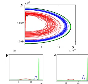
If the noise intensity is small enough, such bundle has a small dispersion and is localized near the deterministic cy-cle (green lines in Fig. 5a). As the noise intensity increases, along with the natural increase of dispersion, the follow-ing unexpected phenomenon is observed: the bundle’s right side of stochastic trajectories is shifted inside the determin-istic cycle (blue and red lines in Fig. 5a). Some details of the corresponding probabilistic distributions are presented in Figs. 5a, b. The probability density functions of u coordi-nates of intersection points of the random trajectories with the linep=1.2935×107Pa are plotted for three values of theF-noise intensity in Fig. 5b whereas the probability den-sity functions of time intervals between successive intersec-tions are shown in Fig. 5c. As one can see, with increasing noise, both the amplitude and period of stochastic oscilla-tions decrease.

This stochastic phenomenon can be explained by the phase portrait peculiarities of an initial deterministic system (see Fig. 2b) near the upper part of vertical fragment of the cycle. In the deterministic case, the phase trajectory slowly moves along the vertical part of the cycle up to pointC. At point C, this trajectory abruptly changes the direction, and begins to move along the arc part quickly. Under the stochastic dis-turbances, random trajectories deviate from this vertical part of the deterministic cycle. As a result of this deviation, the random trajectory can cross the red pseudo-separatrix, and then it falls within the region of large arc-form excursions. In this case, the random trajectory turns right before point C. The more noise, the earlier this turn. Such stochastic de-formation of the random flow results in a decrease ofu- and p-oscillation amplitudes and of the period.

Under the further increase of noise intensity, random states of the system (Eqs. 2, 3, 6) are localized and leave the interior of the deterministic cycle. This noise-induced shift is demon-strated in Fig. 6. Here, an essential decrease of the dispersion of thepcoordinate is observed. In other words,pstabilizes near its certain value with increase in the noise intensity.

The dynamics of plug displacement is shown in Fig. 7. If the noise intensity is large enough so that the system leaves its cycle, the plug displacement increases with noise. If the system is within its cycle, the displacement is also within the corresponding deterministic stepwise curve (black line in Fig. 7).

equa-D. Alexandrov et al.: Stochastic volcanic model 201

(a)

5 10

x 10−4 1.2934

1.2935 x 107

p

u

(b)

5 10

x 10−4

u

P

(c) 40 60

T

P

Figure 5.Stochastic cycles forε= 10−6_{(green),ε= 10}−5_{(blue), andε= 5×10}−5_{(red):(a)random}

trajec-toriesp(Pa) vs.u(m s−1_{),(b)probability density functions ofucoordinates (m s}−1_{),(c)probability density}

functions of the periodT(s).

0 5 10

x 10−4 1.2925

1.293 1.2935

x 107

p

u

Figure 6.Random trajectoriesp(Pa) vs.u(m s−1) forε= 10−4(blue),ε= 5×10−4(red),ε= 7×10−4 (brown), andε= 10−3_{(green). The open circle designates the point of unstable equilibrium.}

12

Figure 5. Stochastic cycles forε=10−6(green),ε=10−5(blue), andε=5×10−5(red): (a) random trajectoriesp(Pa) vs.u(m s−1),

(b) probability density functions ofucoordinates (m s−1), and (c) probability density functions of the periodT (s).

0 5 10

x 10−4 1.2925

1.293 1.2935

x 107

p

u

Figure 6. Random trajectoriesp(Pa) vs.u(m s−1) forε=10−4 (blue), ε=5×10−4 (red), ε=7×10−4 (brown), andε=10−3 (green). The open circle designates the point of unstable equilib-rium.

tions: dp

dt = − 1 V (α1+α2)

[Au−Qeα1(p−p0)_]

+ δ

V (α1+α2)

Qeα1(p−p0)_{ξ(t ), (7)}

0 200 400 600 800 0

0.02 0.04 0.06 0.08

t

d

Figure 7. Displacementd(m) as a function of timet(s) under the influence ofF noise: deterministic case (black),ε=10−4(blue),

ε=5×10−4(red), andε=10−3(green).

dV dt =

α1 α1+α2

[Au−Qeα1(p−p0)_]

− δα1

α1+α2

202 D. Alexandrov et al.: Stochastic volcanic model

0

200

400

600

800

0

0.02

0.04

0.06

0.08

t

d

Figure 7.

Displacement

d

(m) as a function of time

t

(s) under the influence of

F

-noise: deterministic case

(black),

ε

= 10

(blue),

ε

= 5

×

10

(red), and

ε

= 10

(green).

(a)

0 5 10

x 10−4 1.2934

1.2935 x 107

u

p

(b)

0 5 10

x 10−4 1.2934

1.2935 x 107

u

p

(c)

0 5 10

x 10−4 1.2934

1.2935 x 107

p

u

Figure 8.

Stochastic cycles

p

(Pa) vs.

u

(

m s

) for

δ

= 0

.

1

(a)

,

δ

= 0

.

5

(b)

, and

δ

= 2

(c)

.

13

Figure 8. Stochastic cyclesp (Pa) vs.u (m s−1) forδ=0.1 (a),

δ=0.5 (b), andδ=2 (c).

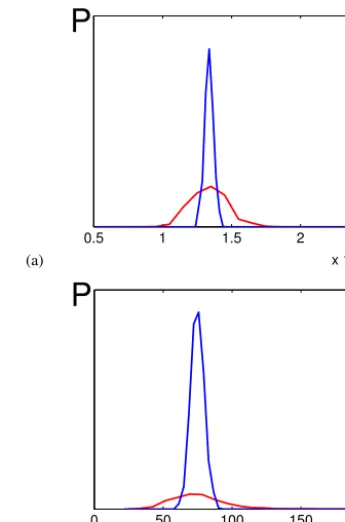
For weak noise, stochastic trajectories are localized near the deterministic cycle (Fig. 8a). As noise intensity in-creases, the dispersion of random trajectories increases as well (Figs. 8b, c). It can be seen that the dispersion is ex-tremely nonuniform along the cycle. For the vertical part, a dispersion is small even for large noise, and the random trajectories do not differ from the deterministic cycle. Along the arc part, the dispersion of the random trajectories in-creases. The probability density functions ofu coordinates of intersection points of the random trajectories with the line

(a)

0.5 1 1.5 2

x 10−3

u

P

(b)

50 100

0 150

T

P

Figure 9.Influence ofQ-noise forδ= 0.5(blue), andδ= 2(red):(a)probability density functions ofu coor-dinates (m s−1_{),(b)probability density functions of the periodT(s).}

14

Figure 9. Influence ofQnoise forδ=0.5 (blue), andδ=2 (red):

(a) probability density functions ofucoordinates (m s−1), (b) prob-ability density functions of the periodT (s).

p=1.2935×107Pa are plotted for three values of theQ -noise intensity in Fig. 9a. Panel b of this figure shows the probability density functions of time intervals between suc-cessive intersections. As one can see, the dispersions grow and the mean values are practically unchangeable with in-creasing noise.

As one can see, the volcanic model under consideration demonstrates quite different qualitative and quantitative re-sponses to the random perturbations of different parameters. The system is extremely sensitive toF noise so that even a weakF noise implies a crucial deformation of the oscilla-tory behavior. An increase ofF noise leads to a decrease of the period and amplitude of oscillations. Note that the sys-tem is also sensitive toQnoise so that a large noise intensity implies a dispersion increase of the arc part of stochastic os-cillations.

4 Conclusions

D. Alexandrov et al.: Stochastic volcanic model 203

state in course of a long time interval. An important point of the deterministic behavior is that a certain constant value of the plug velocityuestablishes at different pressurespin the state of equilibrium (thick vertical line in Fig. 2b). This equilibrium state also persists at different conduit volumesV0 (Fig. 4). A time of system transition to its equilibrium state (vertical line in Fig. 4a) therewith increases with increasing V0. In addition, more broad conduits might have a rather big variation in uandp than more narrow ones during the de-terministic process of the volcanic plug evolution. By this is meant that a time required to attain the equilibrium state in-creases by increasing the conduit’s cross-sectional area.

In order to analyze the role of variations of two main pa-rameters of the plug motion (friction force F and magma influx Q), two types of noises have been introduced in the model equations: F noise andQ noise. It was shown that these noises lead to different evolutionary types of the dy-namic system. Let us summarize the main aspects of this be-havior. In the first place, random trajectories are scattered ei-ther on both sides of the deterministic cycle (Qnoise) or on its internal side (F noise). Dispersions corresponding to ran-dom trajectories of both noises upon that grow by increasing the noise intensities. As this takes place, one can see that both dispersions are highly inhomogeneous along cycles (Figs. 5, 8). Note that these dispersions are small enough in the verti-cal parts of corresponding cycles forF andQnoises.

An important point is that an increase in dispersion occurs in the vicinity of the pseudo-separatrix under the influence ofF noise. This is due to the fact that phase trajectories in-tersect the pseudo-separatrix and the phase points undergo transitions across it under the action of F noise. Let us es-pecially emphasize thatF-noise-phase trajectories leave the corresponding deterministic cycle and form a stochastic bun-dle shifted into the cycle’s interior. As this takes place, the bundle’s dispersion increases while the period and amplitude of oscillations decrease by increasing theF-noise intensity (Fig. 5). By this is meant that the presence of F noise re-duces possible variations in the plug velocity u and pres-surepand decreases a time required to attain the equilibrium state (thick vertical line in Fig. 5a). It is significant that the effect of pressure stabilization near a certain value (depen-dent of the noise intensity) occurs with a rise in theF-noise intensity. The random trajectories therewith leave the corre-sponding cycle and are localized in the vicinity of this value (Fig. 6). A dynamic behavior of the plug displacement is de-pendent of whether the dynamic system is within or beyond its phase cycle. In the former case, the plug displacement os-cillates within the bounds of the corresponding deterministic stepwise curve (Fig. 7). In the latter case, when the noise in-tensity is sufficiently large, the plug displacement increases drastically.

It is known that the eruption of Mount St. Helens was ac-companied by rather regular repetitive long-period (or beat) earthquakes over a long time. Moreover, such drum-beat events were more random from time to time. In addition,

subevents in the form of randomly occurring series of smaller seismic events (produced by a separate random process) have been imposed upon these long-period events (Matoza and Chouet, 2010). The present study demonstrates that repetitive stick–slip motions of the plug representing stochastic oscilla-tions can be connected with these drumbeat earthquakes. The calculated period between drumbeats (see Figs. 5 and 9) is in agreement with experimental data (30–300 s, Iverson et al., 2006). The physical reason is that such earthquakes observed at shallow depths (<1 km at MSH) can be caused by the stick–slip motions of the magma-plug system under the influ-ence of noises where the driving force acting on a compliant crustal body is large enough (the force drop responsible for this kind of seismicity can be estimated from our calculations as1F=1pA∼6×107kg m s−2, where1p∼2×103Pa).

Acknowledgements. This work was supported by the Ministry

of Education and Science of the Russian Federation under the project no. 315.

Edited by: R. Gloaguen

Reviewed by: C. Michaut and G. Wake

References

Alexandrov, D. V., Bashkirtseva, I. A., Malygin, A. P., and Ryashko, L. B.: Sea ice dynamics induced by external stochastic fluctuations, Pure Appl. Geophys., 170, 2273–2282, 2013. Alexandrov, D. V., Bashkirtseva, I. A., and Ryashko, L. B.:

Stochas-tically driven transitions between climate attractors, Tellus A, 66, 23454, doi:10.3402/tellusa.v66.23454, 2014.

Arathi, S., Rajasekar, S., and Kurths, J.: Stochastic and co-herence resonances in a modified chua’s circuit system with multi-scroll orbits, Int. J. Bifurcat. Chaos, 23, 1350132, doi:10.1142/S0218127413501320, 2013.

Barmin, A., Melnik, O., and Sparks, R. S. J.: Periodic behavior in lava dome eruptions, Earth Planet. Sc. Lett., 199, 173–184, 2002. Bashkirtseva, I., Chen, G., and Ryashko, L.: Analysis of noise-induced transitions from regular to chaotic oscillations in the Chen system, Chaos, 22, 033104, doi:10.1063/1.4732543, 2012. Bashkirtseva, I., Neiman, A. B., and Ryashko, L.: Stochas-tic sensitivity analysis of the noise-induced excitability in a model of a hair bundle, Phys. Rev. E, 87, 052711, doi:10.1103/PhysRevE.87.052711, 2013.

Bebbington, M. S. and Marzocchi, W.: Stochastic models for earth-quake triggering of volcanic eruptions, J. Geophys. Res., 116, B05204, doi:10.1029/2010JB008114, 2011.

Costa, A., Wadge, G., and Melnik, O.: Cyclic extrusion of a lava dome based on a stick-slip mechanism, Earth Planet. Sci. Lett., 337–338, 39–46, 2012.

Denlinger, R. P. and Hoblitt, R. P.: Cyclic behavior of cilicic volca-noes, Geology, 27, 459–462, 1999.

Horsthemke, W. and Lefever, R.: Noise-Induced Transitions: The-ory and Applications in Physics, Chemistry, and Biology, Springer, Berlin, 1984.

Iverson, R. M., Dzurisin, D., Gardner, C. A., Gerlach, T. M., LaHusen, R. G., Lisowski, M., Major, J. J., Malone, S. D., Messerich, J. A., Moran, S. C., Pallister, J. S., Qamar, A. I., Schilling, S. P., and Vallance, J. W.: Dynamics of seismogenic volcanic extrusion at Mount St Helens in 2004–05, Nature, 444, 439–443, 2006.

Lai, Y. C. and Tél, T.: Transient Chaos: Complex Dynamics on Fi-nite Time Scales, Springer, Berlin, 2011.

Lindner, B., Garcia-Ojalvo, J., Neiman, A., and Schimansky-Geier, L.: Effects of noise in excitable systems, Phys. Rep., 392, 321–424, 2004.

Matoza, R. S. and Chouet, B. A.: Subevents of long-period seismic-ity: Implications for hydrothermal dynamics during the 2004– 2008 eruption of Mount St. Helens, J. Geophys. Res., 115, B12206, doi:10.1029/2010JB007839, 2010.

McDonnell, M. D., Stocks, N. G., Pearce, C. E. M., and Ab-bott, D.: Stochastic Resonance: from Suprathreshold Stochastic Resonance to Stochastic Signal Quantization, Cambridge Uni-versity Press, Cambridge, 2008.

Melnik, O. E. and Sparks, R. S. J.: Nonlinear dynamics of lava dome extrusion, Nature, 402, 37–41, 1999.

Michaut, C., Ricard, Y., Bercovici, D., and Sparks, R. S. J.: Eruption cyclicity at silicic volcanoes potentially caused by magmatic gas waves, Nat. Geosci., 6, 856–860, 2013.

Moore, P. L., Iverson, N. R., and Iverson, R. M.: Frictional proper-ties of the Mount St Helens gouge, US Geological Survey Pro-fessional Paper 1750, US Geological Survey, Reston, Virginia, 2008.

Nakanishi, M. and Koyaguchi, T.: A stability analysis of a conduit flow model for lava dome eruptions, J. Volcanol. Geoth. Res., 178, 46–57, 2008.

Pikovsky, A. S. and Kurths, J.: Coherence resonance in a noise-driven excitable system, Phys. Rev. Lett., 78, 775–778, 1997. Saltzman, B.: Dynamical Paleoclimatology: Generalised Theory of

Global Climate Change, Academic Press, San Diego, 2002. Sparks, R. S. J.: Forecasting volcanic eruptions, Earth Planet. Sci.

Lett., 210, 1–15, 2003.

Tanaka, H. K. M., Kusagaya, T., and Shinohara, H.: Radiographic visualization of magma dynamics in an erupting volcano, Nat. Commun., 5, 3381, doi:10.1038/ncomms4381, 2014.