https://doi.org/10.5194/npg-25-565-2018 © Author(s) 2018. This work is distributed under the Creative Commons Attribution 4.0 License.
Ensemble variational assimilation as a probabilistic estimator –
Part 1: The linear and weak non-linear case
Mohamed Jardak1,2and Olivier Talagrand1
1LMD/IPSL, CNRS, ENS, PSL Research University, 75231, Paris, France
2Data Assimilation and Ensembles Research & Development Group, Met Office, Exeter, Devon, UK Correspondence:Mohamed Jardak ([email protected])
Received: 17 January 2018 – Discussion started: 24 January 2018
Revised: 3 July 2018 – Accepted: 19 July 2018 – Published: 24 August 2018
Abstract. Data assimilation is considered as a problem in Bayesian estimation, viz. determine the probability distri-bution for the state of the observed system, conditioned by the available data. In the linear and additive Gaussian case, a Monte Carlo sample of the Bayesian probability distribu-tion (which is Gaussian and known explicitly) can be ob-tained by a simple procedure: perturb the data according to the probability distribution of their own errors, and perform an assimilation on the perturbed data. The performance of that approach, called here ensemble variational assimilation (EnsVAR), also known as ensemble of data assimilations (EDA), is studied in this two-part paper on the non-linear low-dimensional Lorenz-96 chaotic system, with the assimi-lation being performed by the standard variational procedure. In this first part, EnsVAR is implemented first, for reference, in a linear and Gaussian case, and then in a weakly non-linear case (assimilation over 5 days of the system). The perfor-mances of the algorithm, considered either as a probabilis-tic or a determinisprobabilis-tic estimator, are very similar in the two cases. Additional comparison shows that the performance of EnsVAR is better, both in the assimilation and forecast phases, than that of standard algorithms for the ensemble Kalman filter (EnKF) and particle filter (PF), although at a higher cost. Globally similar results are obtained with the Kuramoto–Sivashinsky (K–S) equation.
1 Introduction
The purpose of assimilation of observations is to reconstruct as accurately as possible the state of the system under obser-vation, using all the relevant available information. In
geo-physical fluid applications, such as meteorology or oceanog-raphy, that relevant information essentially consists of the physical observations and of the physical laws which govern the evolution of the atmosphere or the ocean. Those physi-cal laws are in practice available in the form of a discretized numerical model. Assimilation is therefore the process by which the observations are combined together with a numer-ical model of the dynamics of the observed system in order to obtain an accurate description of the state of that system.
All the available information, the observations as well as the numerical model, is affected (and, as far as we can tell, will always be affected) with some uncertainty, and one may wish to quantify the resulting uncertainty in the output of the assimilation process. If one chooses to quantify uncertainty in the form of probability distributions (see e.g. Jaynes, 2004, or Tarantola, 2005, for a discussion of the problems which underlie that choice), assimilation can be stated as a prob-lem in Bayesian estimation. Namely, determine the proba-bility distribution for the state of the observed system, con-ditioned by the available information. That statement makes sense only under the condition that the available information is described from the start in the form of probability distri-butions. We will not discuss here the difficult problems as-sociated with that condition (see Tarantola, 2005, for such a discussion) and will assume below that it is verified.
Now, the very large dimension of the numerical models used in meteorology and oceanography (that dimension can lie in the range 106 to 109) forbids explicit description of probability distributions in the corresponding state spaces. A widely used practical solution is to describe the uncertainty in the form of an ensemble of points in state space, with the dispersion of the ensemble being meant to span the uncer-tainty. Two main classes of algorithms for ensemble assimi-lation exist at present. The ensemble Kalman filter (EnKF), originally introduced by Evensen (1994) and further stud-ied by many authors (Evensen, 2003 and Houtekamer and Mitchell, 1998, 2001), is a heuristic extension to large dimen-sions of the standard Kalman filter (KF) Kalman (1960). The latter exactly achieves Bayesian estimation in the linear and Gaussian case that has just been described. It explicitly de-termines the expectation and covariance matrix of the (Gaus-sian) conditional probability distribution and evolves those quantities in time, updating these with new observations as they become available.
The EnKF, contrary to the standard KF, evolves an ensem-ble of points in state space. One advantage is that it can be readily, if empirically, implemented on non-linear dynamics. On the other hand, it keeps the same linear Gaussian proce-dure as KF for updating the current uncertainty with new ob-servations. EnKF exists in many variants and, even with en-semble sizes of relatively small size (O(10–100)), produces results of high quality. It has now become, together with vari-ational assimilation, one of the two most powerful algorithms used for assimilation in large-dimension geophysical fluid applications.
Concerning the Bayesian properties of EnKF, Le Gland et al. (2011) have proven that, in the case of linear dynam-ics and in the limit of infinite ensemble size, EnKF achieves Bayesian estimation, in that it determines the exact (Gaus-sian) conditional probability distribution. In the case of non-linear dynamics, EnKF has a limiting probability distribu-tion, which is not in general the Bayesian conditional distri-bution.
Contrary to EnKF, which was from the start developed for geophysical applications (but has since extended to other fields), particle filters (PFs) have been developed totally in-dependently of such applications. They are based on gen-eral Bayesian principles and are thus independent of any hy-pothesis of linearity or Gaussianity (see Doucet et al., 2000, 2001, and van Leeuwen, 2017, for more details). Like the EnKF, they evolve an ensemble of (usually weighted) points in state space and update them with new observations as these become available. They exist in numerous variants, many of which have been mathematically proven to achieve Bayesianity in the limit of infinite ensemble size (Crisan and Doucet, 2002). On the other hand, no results exist to the au-thors’ knowledge in the case of finite ensemble size. They are actively studied in the context of geophysical applica-tions as presented in van Leeuwen (2009, 2017), but have
not at this stage been operationally implemented on large-dimension meteorological or oceanographical models.
There exist at least two other algorithms that can be uti-lized to build a sample of a given probability distribution. The first one is the acceptance–rejection algorithm described in Miller et al. (1999). The other one is the Metropolis–Hastings algorithm (Metropolis et al., 1953), which itself possesses a number of variants (Robert, 2015). These algorithms can be very efficient in some circumstances, but it is not clear at this stage whether they could be successfully implemented in large-dimension geophysical applications.
Coming back to the linear and Gaussian case, not only, as said above, is the (Gaussian) conditional probability distribu-tion explicitly known, but a simple algorithm exists for deter-mination of independent realizations of that distribution. In succinct terms, perturb additively the data according to their own error probability distribution, and perform the assimila-tion for the perturbed data. Repetiassimila-tion of this procedure on successive sets of independently perturbed data produces a Monte Carlo sample of the Bayesian posterior distribution.
The present work is devoted to the study of that algorithm, and of its properties as a Bayesian estimator, in non-linear and/or non-Gaussian cases. Systematic experiments are per-formed on two low-dimensional chaotic toy models, namely the model defined by Lorenz (1996) and the Kuramoto– Sivashinsky (K–S) equation (Kuramoto and Tsuzuki, 1975, 1976). Variational assimilation, which produces the Bayesian expectation in the linear and Gaussian case, and is routinely, and empirically, implemented in non-linear situations in op-erational meteorology, is used for estimating the state vector for given (perturbed) data. The algorithm is therefore called ensemble variational assimilation, abbreviated to EnsVAR.
This algorithm is not new. There exist actually a rather large number of algorithms for assimilation that are varia-tional (at least partially) and build (at least at some stage) an ensemble of estimates of the state of the observed sys-tem. A review of those algorithms has been recently given by Bannister (2017). Most of these algorithms are actually different from the one that is considered here. They have not been defined with the explicit purpose of achieving Bayesian estimation and are not usually evaluated in that perspective.
EnsVAR, as defined here, has been specifically studied un-der various names and in various contexts by several authors (Oliver et al., 1996; Bardsley, 2012; Bardsley et al., 2014; Liu et al., 2017). Bardsley et al. (2014) have extended it in to what they call the randomize-then-optimize (RTO) algo-rithm. These works have shown that EnsVAR is not in gen-eral Bayesian in the non-linear case, but can nevertheless lead to a useful estimate.
(EDA) for defining the background error covariance matrix of the variational assimilation system. And ECMWF, in its latest reanalysis project ERA5 (Hersbach and Dee, 2016) uses a low-resolution ensemble of data assimilations system in order to estimate the uncertainty in the analysis.
None of the above ensemble methods seems however to have been systematically and objectively evaluated as a prob-abilistic estimator. That is precisely the object of the present two papers.
The first of these is devoted to the exactly linear and weakly linear cases, and the second to the fully non-linear case. In this first one, Sect. 2 describes in detail the EnsVAR algorithm, as well as the experimental set-up that is to be used in both parts of the work. Section 3 describes the statistical tests to be used for objectively assessing EnsVAR as a probabilistic estimator. EnsVAR is implemented in Sect. 4, for reference, in an exactly linear and Gaussian case in which theory says it achieves exact Bayesian estimation. It is implemented in Sect. 5 on the non-linear Lorenz sys-tem, over a relatively short assimilation window (5 days), over which the tangent linear approximation remains basi-cally valid and the performance of the algorithm is shown not to be significantly altered. Comparison is made in Sect. 6 with two standard algorithms for EnKF and PF. Experiments performed on the Kuramoto–Sivashinsky equation are sum-marized in Sect. 7. Partial conclusions, valid for the weakly non-linear case, are drawn in Sect. 8.
The second part is devoted to the fully non-linear situation, in which EnsVAR is implemented over assimilation windows for which the tangent linear approximation is no longer valid. Good performance is nevertheless achieved through the tech-nique of quasi-static variational assimilation (QSVA), de-fined by Pires et al. (1996) and Järvinen et al. (1996). Com-parison is made again with EnKF and PF.
The general conclusion of both parts is that EnsVAR can produce good results which, in terms of performance as a probabilistic estimator and of numerical accuracy, are at least as good as the results of EnKF and PF.
In the sequel of the paper we denote byN(m,P)the multi-variate Gaussian probability distribution with expectationm and covariance matrixP(for a univariate Gaussian probabil-ity distribution, we will use the similar notationN(m, r)).E
will denote statistical expectation, andVar will denote
vari-ance.
2 The method of ensemble variational assimilation We assume the available data make up a vectorz, belonging to data spaceDwith dimensionNz, of the form
z=0x+ζ. (1)
In this expression,xis the unknown vector to be determined, belonging to state spaceS with dimensionNx, while0is a
known linear operator fromSintoD, called the data operator
and represented by anNz×Nx matrix. As for theNzvector
ζ, we will call it an “error”, even though it may not represent an error in the usual sense, but any form of uncertainty. It is assumed to be a realization of the Gaussian probability distributionN(0,6)(in case the expectationE(ζ)were
non-zero, but known, it would be necessary to first unbias the data vectorz by subtracting that expectation). It should be stressed that all available information aboutx is assumed to be included in the data vectorz. For instance, if one, or even several, Gaussian prior estimatesN(xb,Pb)are available for
x, they must be introduced as subsets ofz, each with Nx
components, in the form
xb=x+ζb, ζb∼N(0,Pb).
In those conditions the Bayesian probability distribution
P (x|z)for x conditioned byz is the Gaussian distribution
N(xa,Pa)with
xa=(0T6−10)−10T6−1z
Pa=(0T6−10)−1 . (2)
At first glance, the above equations seem to require the in-vertibility of theNz×Nzmatrix6and then of theNx×Nx
matrix0T6−10. Without going into full details, the need for invertibility of6 is only apparent, and invertibility of
0T6−10is equivalent to the condition that the data operator
0is of rankNx. This in turn means that the data vectorz
con-tains information on every component ofx. This condition is known as the determinacy condition. It implies thatNz≥Nx. We will callp=Nz−Nxthe degree of over-determinacy of the system.
The conditional expectationxacan be determined by
min-imizing the following scalar objective function defined on state spaceS
ξ∈S−→J(ξ)=1
2[0ξ−z]
T6−1[0ξ−z]. (3) In addition, the covariance matrixPa is equal to the inverse
of the Hessian ofJ
Pa=
∂2J
∂ξ2 −1
. (4)
In the case where the errorζ, while still being random with expectation0and covariance matrix6, is not Gaussian, the vectorxadefined in Eq. (2) is not the conditional expectation
ofxfor a givenz, but only the least-variance linear estimate, or best linear unbiased estimate (BLUE), ofxfromz. Sim-ilarly, the matrixPa is no longer the conditional covariance matrix ofx for a givenz, but the covariance matrix of the estimation error associated with the BLUE, averaged over all realizations of the errorζ.
variational assimilation. The latter is routinely implemented in a number of major meteorological centres on non-linear dynamical models with non-linear observation operators. For more on minimization of objective functions of Eq. (3) with non-linear0, see e.g. Chavent (2010).
Coming back to the linear and Gaussian case, consider the perturbed data vectorz0=z+ζ0, where the perturbationζ0
has the same probability distributionN(0,6)as the errorζ. It is easily seen that the corresponding estimate
xa0=(0T6−10)−10T6−1z0 (5)
is distributed according to the Gaussian posterior distribu-tionN(xa,Pa)(Eq. 2). This defines a simple algorithm for
obtaining a Monte Carlo sample of that posterior distribu-tion. Namely, perturb the data vectorzaccording to its own error probability distribution, compute the corresponding es-timate (Eq. 5), and repeat the same process with independent perturbations onz.
That is the ensemble variational assimilation, or EnsVAR, algorithm that is implemented below in linear and non-Gaussian situations, with the analogue of the estimate xa0
being computed by minimization of Eq. (3). In general, this procedure, as already mentioned in the introduction, does not achieve Bayesian estimation, but it is interesting to study the properties of the ensembles thus obtained.
Remark.In the case when, the data operator0being linear, the errorζ in Eq. (1) is not Gaussian, the quantityxa0
defined by Eq. (5) has expectationxa(BLUE) and covariance matrix
Pa(see Isaksen et al., 2010). The probability distribution of
the xa0
is in general not Bayesian, but it has the same ex-pectation and covariance matrix as the Bayesian distribution corresponding to a Gaussianζ.
All the experiments presented in this work are of the stan-dard identical twin type, in which the observations to be as-similated are extracted from a prior reference integration of the assimilating model. And all experiments presented in this first part are of the strong-constraint variational assimilation type, in which the temporal sequence of states produced by the assimilation are constrained to satisfy exactly the equa-tions of the assimilating model.
That model, which will emanate from either the Lorenz or the Kuramoto–Sivashinsky equation, will be written as
xt+1=M(xt), (6)
where xt is the model state at time t, belonging to model
space M, with dimension N (in the strong-constraint case considered in this first part, the model spaceMwill be iden-tical with the state space S). For each model, a “truth”, or reference, runxrt has first been produced. A typical (strong-constraint) experiment is as follows.
Choosing an assimilation window [t0, tT] with lengthT
(it is mainly the parameterT that will be varied in the ex-periments), synthetic observations are produced at successive
times(t0< t1< . . . < tk< . . . < tK=tT), of the form
yk=Hkxrk+k, (7)
whereHkis a linear observation operator, andk∼N(0,Rk)
is an observation error. The k’s are taken to be mutually
independent.
The following process is then implemented Nens times
(iens=1,· · ·, Nens).
i. Perturb the observationsyk, k=0, . . ., Kaccording to
(yiensk )0=yk+δk, (8)
whereδk∼N(0,Rk)is an independent realization of
the same probability distribution that has producedk.
The notation0stresses, as in Eq. (5), the perturbed char-acter of(yiensk )0.
ii. Assimilate the perturbed observations yiensk 0
by mini-mization of the following objective function:
ξ0∈M−→Jiens(ξ0)= (9)
1 2
K X
k=0
Hkξk−
yiensk
0T R−k1
Hkξk−
yiensk
0 ,
whereξkis the value at timetkof the solution of Eq. (6)
emanating fromξ0.
The objective function (Eq. 9) is of type (Eq. 3), with the state spaceS being the model spaceM(N=Nx)and the data vectorz consisting of the concatenation of theK+1 perturbed data vectors yiensk 0
.
The process (i)–(ii), repeatedNenstimes, produces an en-semble ofNensmodel solutions over the assimilation window
[t0, tT].
In the perspective taken here, it is not the properties of those individual solutions that matter the most, but the prop-erties of the ensemble considered as a sample of a probability distribution.
The ensemble assimilation process, starting from Eq. (7), is then repeated overNwinassimilation windows of lengthT (taken sequentially along the true solutionxrt).
In variational assimilation as it is usually implemented, the objective function to be minimized contains a so-called back-ground term at the initial timet0of the assimilation window. That term consists, together with an associated error covari-ance matrix, of a climatological estimate of the model state vector, or of a prior estimate of that vector at timet0 com-ing from assimilation of previous observations. An estimate of the state vector att0 is explicitly present in Eq. (9), in the form of the perturbed observation yiens0 0
The covariance matrixRkin Eq. (9) is the same as the
co-variance matrix of the perturbationsδkin Eq. (8). The situa-tion in which one used in the assimilasitua-tion assumed statistics for the observation errors that were different from the real statistics has not been considered.
We sum up the description of the experimental proce-dure and define precisely the vocabulary to be used in the sequel. The output of one experiment consists of Nwin en-semble variational assimilations. Each enen-semble variational assimilation produces, throughNens minimizations of form (Eq. 9), or individual variational assimilations, an ensemble ofNensmodel solutions corresponding to one set of observa-tionsyk(k=0,· · ·, K)over one assimilation window. These model solutions will be simply called the elements of the ensemble. The various experiments will differ through vari-ous parameters and primarily the lengthT of the assimilation windows.
The minimizations (Eq. 9) are performed through an iter-ative limited-memory BFGS (Broyden–Fletcher–Goldfarb– Shanno) algorithm (Nocedal and Wright, 2006), started from the observationy0at timet0(which, as said below, is taken here as bearing on the entire state vector xr0). Each step of the minimization algorithm requires the explicit knowledge of the local gradient of the objective functionJienswith re-spect toξ0. That gradient is computed, as usual in variational assimilation, through the adjoint of Eq. (6). Unless speci-fied otherwise, the size of the assimilation ensembles will beNens=30, and the numberNwinof ensemble variational assimilations for one experiment will be equal to 9000.
3 The validation procedure
We recall the general result that, among all deterministic functions from data space into state space, the conditional expectationz→E(x|z)minimizes the variance of the esti-mation error onx.
What should ideally be done here for the validation of re-sults is objectively assess (if not on a case-by-case basis, at least in a statistical sense) whether the ensembles produced by EnsVAR are samples of the corresponding Bayesian prob-ability distributions. In the present setting, where the proba-bility distribution of the errors k in Eq. (7) is known, and
where a prior probability distribution is also known, through the observationy0, for the state vectorx0, one could in prin-ciple obtain a sample of the exact Bayesian probability dis-tribution by proceeding as follows.
Through repeated independent realizations of the process defined by Eqs. (6) and (7), build a sample of the joint prob-ability distribution for the couple (x, z). That sample can then be read backwards for a givenz and, if large enough, will produce a useful sample estimate of the corresponding Bayesian probability distribution forx. That would actually solve numerically the problem of Bayesian estimation. But it is clear that the sheer numerical cost of the whole process,
which requires explicit exploration of the joint space (x,z), makes this approach totally impossible in any realistic situa-tion.
We have evaluated instead the weaker property of relia-bility (also called calibration). Reliarelia-bility of a probabilistic estimation system (i.e. a system that produces probabilities for the quantities to be estimated) is the statistical consis-tency between the predicted probabilities and the observed frequencies of occurrence.
Consider a probability distributionπ(the words probabil-ity distribution must be taken here in the broadest possible sense, meaning as well discrete probabilities for the occur-rence of a binary or multi-outcome event, as continuous dis-tributions for a one- or multi-dimensional random variable), and denoteπ0(π )the distribution of the reality in the circum-stances whenπhas been predicted. Reliability is the property that, for anyπ, the distributionπ0(π )is equal toπ.
Reliability can be objectively evaluated, provided a large enough verification sample is available. Bayesianity clearly implies reliability. For any data vectorz, the true state vec-torx is distributed according to the conditional probability distributionP (x|z), so that a probabilistic estimation system which always producesP (x|z)is reliable. The converse is clearly not true. A system which, ignoring the observations, always produces the climatological probability distribution for x will be reliable. It will however not be Bayesian (at least if, as one can reasonably hope, the available data bring more than climatological information on the state of the sys-tem).
Another desirable property of a probabilistic estimation system, although not directly related to Bayesianity, is res-olution (also called sharpness). It is the capacity of the sys-tem for a priori distinguishing between different outcomes. For instance, a system which always predicts the climato-logical probability distribution is perfectly reliable, but has no resolution. Resolution, like reliability, can be objectively evaluated if a large enough verification sample is available.
−5 −4.5 −4 −3.5 −3 −2.5 −2 −1.5 −1 −0.5 0 0.02
0.03 0.04 0.05 0.06 0.07 0.08 0.09 0.1
Time (days)
Errors
Observation error SD
Mean error Error mean
Raw assimilation error
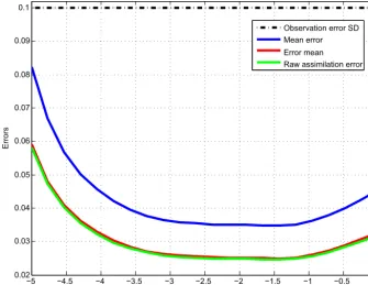
Figure 1.Root-mean-square errors from the truth as functions of time along the assimilation window (linear and Gaussian case). Blue curve: error in individual minimizations. Red curve: error in the means of the ensembles. Green curve: error in the assimilations performed with the unperturbed observationsyk(Eq. 7). Dashed–dotted horizontal curve: standard deviation of the observation error. Each point on the blue curve corresponds to an average over a sample ofNx·Nwin·Nens=1.08×10⁷elements and each point on the red and green curves to an
average over a sample ofNx·Nwin=3.6×10⁵elements.
on objective validation of probabilistic estimation systems, see e.g. chap. 8 of the book by Wilks (2011), as well as the papers by Talagrand et al. (1997) and Candille and Talagrand (2005).
4 Numerical results: the linear case
We present in this section results obtained in an exactly lin-ear and Gaussian case, in which theory says that EnsVAR must produce an exact Monte Carlo Bayesian sample. These results are to be used as a benchmark for the evaluation of later results. The numerical model (Eq. 6) is obtained by lin-earizing the non-linear Lorenz model, which describes the space–time evolution of a scalar variable denoted x, about one particular solution (the Lorenz model will be described and discussed in more detail in Sect. 5; see Eq. 12 below). The model space dimensionN is equal to 40. The lengthT
of the assimilation windows is 5 days, which coversNt=20
timesteps (the “day” will be defined in the next section). The complete state vector (Hk=I in Eq. 7) is observed every
0.5 days(K=10). The data vectorzhas therefore dimension
(K+1)N=440. The observation errors are Gaussian, spa-tially uncorrelated, with constant standard deviationσ=0.1
(Rk=σ2I,∀k). However, because of the linearity, the
abso-lute amplitude of those errors must have no impact.
Since conditions for exact Bayesianity are verified, any de-viation in the results from exact reliability can be due to only the finitenessNensof the ensembles (except for the rank his-togram, which takes that finiteness into account), the finite-nessNwinof the validation sample, or numerical effects (such as resulting from incomplete minimization or round-off er-rors).
Bins
0 5 10 15 20 25 30
Frequency
0 0.1 0.2 0.3 0.4 0.5 0.6 0.7 0.8 0.9 1
Rank histogram
Predicted probability
0 0.2 0.4 0.6 0.8 1
Observed relative frequency
0 0.1 0.2 0.3 0.4 0.5 0.6 0.7 0.8 0.9
1 Reliability diagram
Threshold
-1 -0.8 -0.6 -0.4 -0.2 0 0.2 0.4 0.6 0.8 1
Log(brier scores)
10-4
10-3
10-2
10-1 Brier scores
Resolution Reliability
(a) (b)
(c)
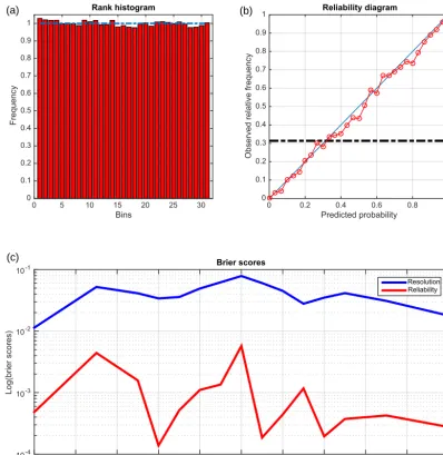
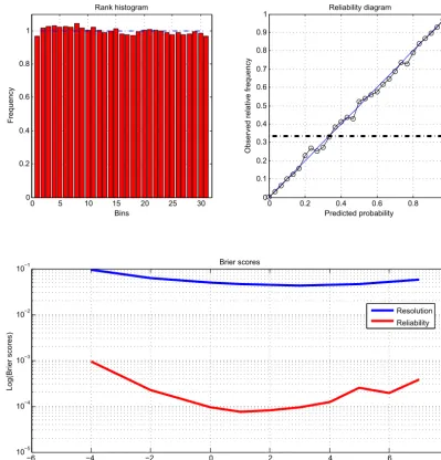
Figure 2.Diagnostics of statistical performance (linear and Gaussian case).(a)Rank histogram for the model variablex.(b)Reliability diagram for the eventE= {x >1.14}(black horizontal dashed–dotted line: frequency of occurrence of the event).(c)Variation with threshold
τ of the reliability and resolution components of the Brier score for the eventsE= {x > τ}(red and blue curves respectively; note the logarithmic scale on the vertical). The diagnostics have been computed over all grid points, timesteps, and realizations, making up a sample of size 7.56×10⁶.
between the values on the blue and green curves, averaged over the whole assimilation window, is equal to 1.414. This is close to
√
2 as can be expected from the linearity of the process and the perturbation procedure defined by Eqs. (7)– (8) (actually, it can be noted that the value
√
2 is itself, in-dependently of any linearity, a test for reliability, since the standard deviation of the difference between two indepen-dent realizations of a random variable must be equal to
√
2 times the standard deviation of the variable itself). The green curve corresponds to the expectation of (what must be) the Bayesian probability distribution, while the red curve cor-responds to a sample expectation, computed overNens
ele-ments. The latter expectation is therefore not, as can be seen on the figure, as accurate an estimate of the truth. The rela-tive difference must be about2N1
ens≈0.017. This is the value obtained here.
For a reliable system, the reduced centred random vari-able, which we denotes, has expectation 0 and variance 1 (see Appendix A). The sample values, computed over all grid points, times, and assimilation windows (which amounts to a set of sizeNx·(Nt+1)·Nwin=7.56×10⁶), areE(s)=0.0035
andVar(s)=1.00.
140 160 180 200 220 240 260 0
100 200 300 400 500 600 700
Histogram Numerical mean Numerical SD
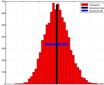
Figure 3.Histogram of (half) the minima of the objective function (Eq. 9), along with the corresponding mean (vertical black line) and standard deviation (horizontal blue line) (linear and Gaussian case).
individual ensembles in the experiment. The top-left panel is the rank histogram. The top-right panel is the reliability diagram relative to the event{x >1.14}, which occurs with frequency 0.32 (black horizontal dashed–dotted line in the diagram). Both panels visually show high reliability (flatness for the histogram, closeness to the diagonal for the reliability diagram), although that reliability is obviously not perfect. More accurate quantitative diagnostics are given by the lower panel, which shows, as functions of the thresholdτ, the two components (reliability and resolution; see Eqs. A4 and A5 respectively) of the Brier score for the events{x > τ}. The re-liability component is about 10−3; the resolution component is about 5×10⁻². A further diagnostic has been made by comparison with an experiment in which the validating truth has been obtained, for each of theNwin windows, from an additional independent(Nens+1)st variational assimilation. That procedure is by construction perfectly reliable, and any difference with Fig. 2 could result only from the fact that the validating truth is not defined by the same process. The reli-ability (not shown) is very slightly improved in comparison with Fig. 2 (this could be possibly due to a lack of full conver-gence of the minimizations). The resolution is not modified. It is known that the minimumJmin=J(xa)of the objec-tive function (Eq. 3) takes on average the value
E(Jmin)=
p
2, (10)
wherep=Nz−Nx has been defined as the degree of over-determinacy of the minimization. This result is true provided the following two conditions are verified: (i) the operator0is linear and (ii) the errorζin Eq. (1) has expectation0and the covariance matrix6used in the objective function (Eq. 3). It is independent of whetherζ is Gaussian or not. But whenζ
is Gaussian, the quantity 2Jminfollows aχ2probability dis-tribution of orderp(for that reason, Eq. 10 is often called the
χ2condition, although it is verified in circumstances where 2Jmindoes not follow aχ2distribution). As a consequence, the minimumJminhas standard deviation
σ(Jmin)=
p
p/2. (11)
In the present case,Nx=40 andNz=(K+1)Nx=440, so
thatp/2=200 and√p/2≈14.14.
The histogram of the minimaJmin(corrected for a mul-tiplicative factor 1/2 resulting from the additional perturba-tions, Eq. 8) is shown in Fig. 3. The corresponding empirical expectation and standard deviation are 199.39 and 14.27 re-spectively, in agreement with Eqs. (10)–(11). It can be noted that, as a consequence of the central limit theorem, the his-togram in Fig. 3 is in effect Gaussian. Indeed the value of negentropy, a measure of Gaussianity that will be defined in the next section, is 0.0012.
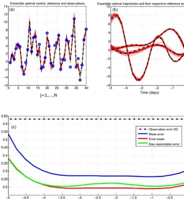
de-Figure 4.Diagnostics relative to the non-linear and Gaussian case, with assimilation over 5 days.(a)and(b)are relative to one particular assimilation window. (a)(horizontal coordinate: spatial positionj) Reference truth at the initial time of the assimilation window (black dashed curve), observations (blue circles), and minimizing solutions (full red curves).(b)(horizontal coordinate: time along the assimilation window) Truth (dashed curve) and minimizing solutions (full red curves) at three points in space.(c)Overall diagnostics of estimation errors (same format as in Fig. 1).
creases (through increased observation error and/or degraded spatial and/or temporal resolution of the observations). Sta-tistical resolution should, on the other hand, be degraded. Ex-periments have been performed to check this aspect (the ex-act experimental procedure is described in Sect. 5). The nu-merical results (not shown) are that both components of the Brier score are actually degraded and can increase by 1 or-der of magnitude. The reliability component always remains much smaller than the resolution component, and the degra-dation of the latter is much more systematic. This is in good agreement with the fact that the degradation of reliability can be due to only numerical effects, such as less efficient mini-mizations.
The above results, obtained in the case of exact theoretical Bayesianity, are going to serve as reference for the evaluation of EnsVAR in non-linear and non-Gaussian situations where Bayesianity does not necessarily hold.
5 Numerical results: the non-linear case
The non-linear Lorenz-96 model (Lorenz, 1996; Lorenz and Emanuel, 1998) reads
dxj
dt = xj+1−xj−2
xj−1−xj+F, (12)
0 5 10 15 20 25 30 0
0.2 0.4 0.6 0.8 1
Bins
Frequency
Rank histogram
0 0.2 0.4 0.6 0.8 1
0 0.1 0.2 0.3 0.4 0.5 0.6 0.7 0.8 0.9 1
Predicted probability
Observed relative frequency
Reliability diagram
−6 −4 −2 0 2 4 6 8
10−5
10−4
10−3
10−2
10−1
Threshold
Log(Brier scores)
Brier scores
Resolution Reliability
Figure 5.Same as Fig. 2, for the non-linear case (for the eventE= {x <1.}, which occurs with frequency 0.33, as concerns the reliability diagram on the top-right panel).
we choose N=40 andF =8. For these values, the model is chaotic with 13 positive Lyapunov exponents, the largest of which has a value of (2.5 day)−1, where 1 day is equal to 0.24 time unit in Eq. (12). This is the definition of “day” we will use hereafter. It is slightly different from the choice made in Lorenz (1996), where the day is equal to 0.2 time unit in Eq. (12). The difference is not critical for the sequel, nor for possible comparison with other works.
Except for the dynamical model, the experimental setup is fundamentally the same as in the linear case. In particu-lar, the model time step 0.25 days (our definition), the ob-servation frequency 0.5 days, and the valuesNens=30 and
Nwin=9000 are the same. The observation error is uncor-related in space and time, with constant variance σ2=0.4
(Rk=σ2I,∀k). The associated standard deviationσ=0.63
is equal to 2 % of the variability of the reference solution (it is because of the different range of variability that the value ofσ has been chosen different from the value in the linear case). We mention again that no cycling is present between successive assimilation windows.
The results are shown on Fig. 4. The top panels are rela-tive to one particular assimilation window. In the left panel, where the horizontal coordinate is the spatial positionj, the black dashed curve is the reference truth at the initial time of the assimilation window, the blue circles are the corre-sponding observations, and the full red curves (Nens=30 of them) are the minimizing solutions at the same time. The right panel, where the horizontal coordinate is time along the assimilation window, shows the truth (dashed curve) and the
differ--6 -4 -2 0 2 4 6 8 Threshold
100
Log(Brier scores)
Impact of the time frequency of observing
-6 -4 -2 0 2 4 6 8
Threshold
100
Log(Brier scores)
Impact of the observation spatial distribution
-6 -4 -2 0 2 4 6 8
Threshold
100
Log(Brier scores)
Impact of the observation error spread (a)
(b)
(c)
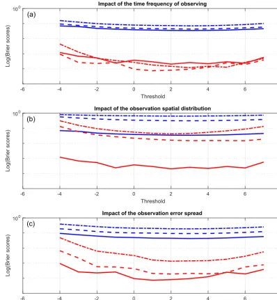
Figure 6.Impact of the informative content of observations on the two components of the Brier score (non-linear case). The format of each panel is the same as the format of the bottom panels of Figs. 2 and 5 (red and blue curves: reliability and resolution components respectively). (a)Impact of the temporal density of the observations. Observations are performed every grid point, with error varianceσ2=0.4; every time step (full curves); and every second and fourth timestep (dashed and dashed–dotted curves respectively).(b)Impact of the spatial density of the observations. Observations are performed every timestep, with errorσ2=0.4; at every grid point (full curves); and every second and fourth grid point (dashed and dashed–dotted curves respectively).(c)Impact of the varianceσ2of the observation error. Observations are performed every second timestep and at every grid point with observation error SDσ=
√ 0.4,2
√
0.4, and 4 √
0.4 (full, dashed, and dashed–dotted curves respectively.
ent points in space. Both panels show that the minimizations reconstruct the truth with a high degree of accuracy.
The bottom panel, which shows error statistics accumu-lated over all assimilation windows, is in the same format as Fig. 1 (note that, because of the different dynamics and ob-servational error, the amplitude on the vertical axis is differ-ent from Fig. 1). The conclusions are qualitatively the same. The estimation error, which is smaller than the observational
error, is maximum at both ends of the assimilation window and minimum at some intermediate time. The ratio between the blue and red curves, equal on average to 1.41, is close to the value
√
2, which, as already said, is in itself an indi-cation of reliability. But a significant difference is that the green curve lies now above the red curve. One obtains a bet-ter approximation of the truth by taking the average of the
assimila-0 1000 2000 3000 4000 5000 6000 7000 8000 9000 0
200 400 600 800 1000 1200 1400 1600 1800
Realizations
Jmin
Jmin
Numerical mean
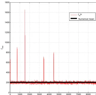
Figure 7. Values of (half) the minima of the objective function for all realizations (non-linear case) (horizontal coordinate: realization number; vertical coordinate: value of the minima).
tion on the raw observations (Eq. 7). This is an obvious non-linear effect. One can note it is fully consistent with the fact that the expectation of the a posteriori Bayesian probability distribution is the variance-minimizing estimate of the truth. The expectation and variance of the RCRV are respectively
E(s)=0.012 andVar(s)=1.047.
Figure 5, which is in the same format as Fig. 2, shows similar diagnostics: rank histogram; reliability diagram for the event{x <1.0}, which occurs with frequency 0.33; and the two components of the Brier score for events of the form
{x > τ}. The general conclusion is the same as in the linear case. High level of reliability is achieved. Actually, the relia-bility component of the Brier score (bottom panel) is now de-creased below 10−3. That improvement, in the present situa-tion where exact Bayesianity cannot be expected, can only be due to better numerical conditioning than in the linear case. The resolution component of the Brier score, on the other hand, is increased.
Figure 6 is relative to experiments in which the informa-tive content of the observations, i.e. their temporal density, spatial density, and accuracy (top, middle, and bottom pan-els respectively), has been varied. Each panel shows the two
0 0.1 0.2 0.3 0.4 0.5 0.6 0.7 0.8 0.9 1
J(
xopt
+
(1-) x
start
)
0 1000 2000 3000 4000 5000 6000 7000 8000 9000
Interpolated quadratic section Objective function section
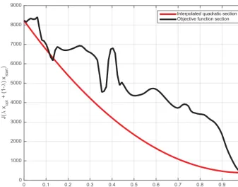
Figure 8.Cross section of the objective functionJiens, for one particular minimization, between the starting point of the minimization and the minimum ofJiens(black curve). Parabola going through the starting point and having the same minimum (red curve).
Figure 7 shows the distribution of (half) the minima of the objective function (it contains the same information as Fig. 3, in a different format). Most values are concentrated around the linear value 200, but a small number of values are present in the range 600–1000. Excluding these outliers, the expec-tation and standard deviation of the minima are 199.62 and 14.13 respectively. These values are actually in better agree-ment with the theoretical χ2 values (200 and 14.14) than the ones obtained above in the theoretically exact Bayesian case (199.39 and 14.27). This again suggests better numeri-cal conditioning for the non-linear situation.
In view of previous results, in particular results obtained by Pires et al. (1996), a likely explanation for the presence of the larger minima in Fig. 7 is the following. Owing to the non-linearity of Eq. (12), and more precisely to the folding which occurs in state space as a consequence of the chaotic character of the motion, the uncertainty in the initial state is distributed along a folded subset in state space. It occasion-ally happens that the minimum of the objective function falls in a secondary fold, which corresponds to a larger value of the objective function. This aspect will be further discussed in the second part of the paper. In any case, the presence of larger minima of the objective function is an obvious sign of non-linearity.
Non-linearity is also obvious in Fig. 8, which shows, for one particular minimization, a cross section of the objective function between the starting point of the minimization and the minimum of the objective function (black curve), as well
as a parabola going through the starting point and having the same minimum (red curve). The two curves are distinctly dif-ferent, while they would be identical in a linear case.
We have evaluated the Gaussian character of univariate marginals of the ensembles produced by the assimilation by computing their negentropy. The negentropy of a probability distribution is the Kullback–Leibler divergence of that dis-tribution with respect to the Gaussian disdis-tribution with the same expectation and variance (see Appendix B). The negen-tropy is positive and is equal to 0 for exact Gaussianity. The mean negentropy of the ensembles is here≈10−3, indicating closeness to Gaussianity (for a reference, the negentropy of the Laplace distribution is 0.072). Although non-linearity is present in the whole process, EnsVAR produces ensembles that are close to Gaussianity.
Experiments have been performed in which the observa-tional error, instead of being Gaussian, has been taken to follow a Laplace distribution (with still the same variance
0 5 10 15 20 25 30 0
0.2 0.4 0.6 0.8 1 1.2
Bins
Frequency
Rank histogram
−5 −4 −3 −2 −1 0
−8 −6 −4 −2 0 2 4 6 8 10
Time (days)
Ensemble optimal trajectories and respective reference solutions
0 0.2 0.4 0.6 0.8 1
0 0.1 0.2 0.3 0.4 0.5 0.6 0.7 0.8 0.9
1 Reliability diagram
Predicted probability
Observed relative frequency
−2 −1 0 1 2 3 4 5 6
10−3 10−2 10−1
Threshold
Log(Brier skill scores)
Brier skill scores
Resolution Reliability
(a) (b)
(c) (d)
Figure 9. (a)Identical with the top-right panel of Fig. 4, repeated for comparison with figures that follow. The other panels show the same diagnostics as in Fig. 5 but performed at the final time of the assimilation windows.(b)Rank histogram.(c)Reliability diagram for the event E= {x >1.33}, which occurs with frequency 0.42.(d)Components of the Brier score for the eventsE= {x > τ}(same format as in the bottom panels of Figs. 2 and 5).
6 Comparison with the ensemble Kalman filter and the particle filter
We present in this section a comparison with results obtained with the ensemble Kalman filter (EnKF) and the particle filter (PF). As used here, those filters are sequential in time. Fair comparison is therefore possible only at the end of the as-similation window. Figure 9 shows the diagnostics obtained from EnsVAR at the end of the window (the top-left panel, identical with the top-right panel of Fig. 4, is included for easy comparison with the figures that will follow).
Compar-ison with Fig. 5 shows that the reliability (as measured by the rank histogram, the reliability diagram, and the reliability component of the Brier score) is significantly degraded. It has been verified (not shown) that this degradation is mostly due not to a really degraded performance at the end of the win-dow, but to the use of a smaller validation sample (by a factor ofNt+1=21, which leads to a sample with size 3.6×10⁵).
updat-0 0.2 0.4 0.6 0.8 1 0
0.1 0.2 0.3 0.4 0.5 0.6 0.7 0.8 0.9 1
Predicted probability
Observed relative frequency
Reliability diagram
−2 −1 0 1 2 3 4 5 6
10−3
10−2
10−1
Threshold
Log(Brier skill scores)
Brier skill scores
Resolution Reliability
0 5 10 15 20 25 30
0 0.2 0.4 0.6 0.8 1 1.2 1.4 1.6
Bins
Frequency
Rank histogram
−5 −4 −3 −2 −1 0
−10 −5 0 5 10 15
Time (days)
EnKF trajectories and respective reference solutions
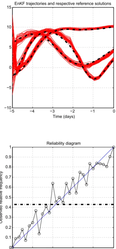
Figure 10.Same as Fig. 9, for the ensemble Kalman filter.
ing the background ensembles, according to the probabil-ity distribution of the observation errors. Spatial localization of the background error covariance matrix has been imple-mented by Schur-multiplying the sample covariance matrix by a squared exponential kernel with length scale 12.0 (the positive definiteness of the periodic kernel has been ensured by removing its negative Fourier components). And multi-plicative inflation with factorr=1.001 has been applied, as in Anderson and Anderson (1999), on the ensemble after each analysis.
Comparison with Fig. 9 shows that the individual ensem-bles, after a warm-up period, tend to remain more dispersed than in EnsVAR (top-left panel). Reliability, as measured by the reliability diagram and the Brier score, is similar to what
it is in Fig. 9. But it is significantly degraded as evaluated by the rank histogram. The ensembles, although they have larger absolute dispersion than in EnsVAR, tend to miss re-ality more often.
Following comments from referees, we have made a few experiments not using localization in the EnKF. The RMSE and the RCRV are significantly degraded, while the rank his-togram and the resolution component of the Brier score are improved. The reliability component of the Brier score re-mained the same. All this is true for both assimilation and forecast. These results, not included in the paper, would de-serve further studies which are postponed for a future work.
−5 −4 −3 −2 −1 0 −15
−10 −5 0 5 10 15
Time (days)
PF trajectories and respective reference solutions
0 0.2 0.4 0.6 0.8 1
0 0.1 0.2 0.3 0.4 0.5 0.6 0.7 0.8 0.9 1
Predicted probability
Observed relative frequency
Brier skill scores
−2 −1 0 1 2 3 4 5 6
10−3 10−2 10−1 100
Threshold
Log(Brier skill scores)
Brier skill scores
Resolution Reliability
0 5 10 15 20 25 30
0 0.2 0.4 0.6 0.8 1 1.2 1.4 1.6
Bins
Frequency
Rank histogram
Figure 11.Same as Fig. 9, for the particle filter.
here is the “Sampling Importance Particle Filter” presented in Arulampalam et al. (2002). Comparison with Fig. 10 shows first that the individual ensembles are still more dis-persed than in EnKF (top-left panel). It also shows a slight degradation of the reliability component of the Brier score (and, incidentally, a significant degradation of the resolu-tion component), but no visible difference on the reliability diagram. Concerning the rank histogram, PF produces un-equally weighted particles, and the standard histogram could not be used. A histogram has been built instead on the quan-tiles defined by the weights of the particles. This shows, as for EnKF, a significant tendency to miss the truth.
The left column of Table 1 shows the mean root-mean-square error in the means of the ensembles as obtained from
Table 1.RMS errors at the end of 5 days of assimilation (left col-umn) and of 5 days of forecast (right colcol-umn) for the three algo-rithms.
Assimilation Forecasting
EnsVAR 0.22 1.49
EnKF 0.24 1.67
PF 0.76 2.63
−5 0 5 −6
−4 −2 0 2 4 6 8
Time (days)
Ensemble optimal trajectories and their respective reference solutions
0 5 10 15 20 25 30
0 0.2 0.4 0.6 0.8 1
Bins
Frequency
Rank histogram
0 0.2 0.4 0.6 0.8 1
0 0.1 0.2 0.3 0.4 0.5 0.6 0.7 0.8 0.9 1
Predicted probability
Observed relative frequency
Reliability diagram
−5 0 5 10
10−3 10−2 10−1 100
Threshold
Log (Brier scores)
Brier scores
Resolution
Reliability
Figure 12.Same as Fig. 9, but at the end of 5-day forecasts. On the top-left panel the horizontal axis spans both the assimilation and the forecast intervals.
Figures 12–14 are relative to ensemble forecasts per-formed, for each of the three assimilation algorithms, from the ensembles obtained at the end of the 5-day assimilations. They are in the same format as Fig. 9 and show diagnostics at the end of 5-day forecasts. One can first observe that the dispersion of individual forecasts (top-left panels) increases, as can be expected, with the forecast range, but much less with the EnsVAR than with EnKF and PF. Reliability, as measured by the Brier score, is slightly degraded in all three algorithms with respect to the case of the assimilations. It is slightly worse for EnKF than for EnsVAR and significantly worse for PF. Resolution is, on the other hand, significantly degraded in all three algorithms. This is associated with the
dispersion of ensembles and corresponds to what could be expected. Concerning the rank histograms, the histogram of EnsVAR, although still noisy, shows no systematic sign of over- or underdispersion of the ensembles. The EnKF and PF histograms both present, as before, what appears to be a significant underdispersion.
−5 0 5 −8
−6 −4 −2 0 2 4 6 8 10 12
Time (days)
Ensemble optimal trajectories and their respective reference solutions
0 5 10 15 20 25 30
0 0.2 0.4 0.6 0.8 1 1.2 1.4
Bins
Frequency
Rank histogram
0 0.2 0.4 0.6 0.8 1
0 0.1 0.2 0.3 0.4 0.5 0.6 0.7 0.8 0.9 1
Predicted probability
Observed relative frequency
Reliability diagram
−5 0 5 10
10−3 10−2 10−1 100
Threshold
Log(Brier scores)
Brier scores
Resolution Reliability
Figure 13.Same as Fig. 12, but for EnKF.
7 The Kuramoto–Sivashinsky equation
Similar experiments have been performed with the Kuramoto–Sivashinsky (K–S) equation. It is a one-dimensional spatially periodic evolution equation, with an advective non-linearity, a fourth-order dissipation term, and a second-order anti-dissipative term. It reads
∂u ∂t +
∂4u ∂x4+
∂2u ∂x2+u
∂u
∂x =0, x∈ [0, L] ∂iu
∂xi(x+L, t )= ∂iu
∂xi(x, t )fori=0,1, . . .,4,∀t >0 u(x,0)=u0(x)
,
(13)
−5 0 5 −10
−5 0 5 10 15
Time (days)
Ensemble optimal trajectories and their respective reference solutions
0 0.2 0.4 0.6 0.8 1
0 0.1 0.2 0.3 0.4 0.5 0.6 0.7 0.8 0.9 1
Predicted probability
Observed relative frequency
Reliability diagram
−5 0 5 10
10−2 10−1 100
Threshold
Log (Brier scores)
Brier scores
Resolution Reliability
0 5 10 15 20 25 30
0 0.2 0.4 0.6 0.8 1 1.2 1.4 1.6
Bins
Frequency
Rank histogram
Figure 14.Same as Fig. 12, but for PF.
WithL=32πand the initial condition
u(x,0)=cosx
16 1+sin
x
16
, (14)
Equation (13) is known to be stiff. The stiffness is due to rapid exponential decay of some modes (the dissipative part) and to rapid oscillations of other modes (the dispersive part). Figure 15, where the two panels are in the same format as Fig. 1, shows the errors in the EnsVAR assimilations, in both a linearized (top panel) and a fully non-linear (bottom panel) cases. The length of the assimilation window, marked as 1 on the figure, is equal to λ1
max ≈7.7 in units of Eq. (13), i.e. a typical predictability time of the system. The shapes of the curves show that the K–S equation has globally more stabil-ity and less instabilstabil-ity than the Lorenz equation. The figure shows similar performance for the linear and non-linear sit-uation. Other results (not shown) are also qualitatively very similar to those obtained with the Lorenz equation: high
re-liability of the ensembles produced by EnsVAR and slightly superior performance over EnKF and PF.
8 Summary and conclusions
Ensemble variational assimilation (EnsVAR) has been imple-mented on two small-dimension non-linear chaotic toy mod-els, as well as on linearized versions of those models.
−1 −0.9 −0.8 −0.7 −0.6 −0.5 −0.4 −0.3 −0.2 −0.1 0 0
0.05 0.1 0.15 0.2
Time
Errors
Linear case
−1 −0.9 −0.8 −0.7 −0.6 −0.5 −0.4 −0.3 −0.2 −0.1 0
0 0.05 0.1 0.15 0.2 0.25 0.3
Nonlinear case
Time
Errors
Observation error SD Mean error Error mean
Observation error SD Mean error Error mean (a)
(b)
Figure 15.Same as Fig. 1, for variational ensemble assimilations performed on the Kuramoto–Sivashinsky equation, i.e. root-mean-square error from the truth along the assimilation window, averaged at each time over all grid points and all realizations, for both the linear and non-linear cases (aandbrespectively).
In view of the impossibility of objectively validating the Bayesianity of ensembles, the weaker property of reliability has been evaluated instead. In the linear and Gaussian case, where theory says that EnsVAR is exactly Bayesian, the re-liability of the ensembles produced by EnsVAR is high, but not numerically perfect, showing the effect of sampling er-rors and, probably, of numerical conditioning.
In the non-linear case, EnsVAR, implemented on temporal windows on the order of magnitude of the predictability time of the systems, shows as good (and in some cases slightly better) performance as in the exactly linear case. Comparison with the ensemble Kalman filter (EnKF) and the particle filter (PF) shows EnsVAR is globally as good a statistical estimator as those two other algorithms.
On the other hand, EnsVAR, at it has been implemented here, is numerically more costly than either EnKF or PF. And the specific algorithms used for the latter two methods
may not be the most efficient. But it is worthwhile to evaluate EnsVAR in the more demanding conditions of stronger non-linearity. That is the object of the second part of this work.
Appendix A: Methods for ensemble evaluation
This Appendix describes in some detail two of the scores that are used for evaluation of results in the paper, namely the re-duced centred random variable and the reliability–resolution decomposition of the classical Brier score. Given a predicted probability distribution for a scalar variablex and a verify-ing observation ξ, the corresponding value of the reduced centred random variable is defined as
s≡ξ−µ
σ , (A1)
whereµ andσ are respectively the mean and the standard deviation of the predicted distribution. For a perfectly reli-able prediction system, and over all realizations of the sys-tem, s, by the very definition of expectation and standard deviation, has expectation 0 and variance 1. This is true in-dependently of whether or not the predicted distribution is always the same. An expectation ofs that is different from 0 means that the system is globally biased. If the expecta-tion is equal to 0, a variance ofsthat is smaller (respectively larger) than 1 is a sign of global overdispersion (respectively underdispersion) of the predicted distribution. One can note that, contrary to the rank histogram, which is invariant in any monotonous one-to-one transformation on the variablex, the RCRV is invariant only in a linear transformation.
We recall the Brier score for a binary eventEis defined by
B=E
h
(p−p0)2
i
, (A2)
where p is the probability predicted for the occurrence of
E in a particular realization of the probabilistic prediction process,p0is the corresponding verifying observation (p0= 1 or 0 depending on whether E has been observed to occur or not), and Edenotes the mean taken over all realizations
of the process. Denoting byp0(p), for any probabilityp, the frequency with whichEis observed to occur in the circum-stances whenphas been predicted,Bcan be rewritten as
B=E
h
(p−p0)2i+Ep0(1−p0). (A3) The first term on the right-hand side, which measures the horizontal dispersion of the points on the reliability diagram about the diagonal, is a measure of reliability. The second term, which is a (negative) measure of the vertical dispersion of the points, is a measure of resolution (the larger the dis-persion, the higher the resolution, and the smaller the second term on the right-hand side). It is those two terms, divided by the constantpc(1−pc), wherepc=E(p0)is the overall observed frequency of occurrence ofE, that are taken in the present paper as measures of reliability and resolution:
Breli=
E(p−p0)2 pc(1−pc)
, (A4)
Breso=
Ep0(1−p0)
pc(1−pc) . (A5)
Both measures are negatively oriented and have 0 as op-timal value.Breli is bounded above by 1/pc(1−pc), while Bresois bounded by 1.
Remark.There exist other definitions of the reliability and resolution components of the Brier score. In particular, con-cerning resolution, the uncertainty termpc(1−pc)(which
depends on the particular eventEunder consideration) is of-ten subtracted from the start from the raw score (Eq. A2). This leads to slightly different scores.
As said in the main text, more on the above diagnostics and, more generally, on objective validation of probabilistic estimation systems can be found in e.g. chap. 8 of the book by Wilks (2011), or in the papers by Talagrand et al. (1997) and Candille and Talagrand (2005).
Appendix B: Negentropy
The negentropy of a probability distribution with density
f (y)is the Kullback–Leibler divergence, or relative entropy, of that distribution with respect to the Gaussian distribution with the same expectation and variance. Denoting byfG(y) the density of that Gaussian distribution, the negentropy can be expressed as
N (f )= Z
f (y)ln
f (y) fG(y)
dy. (B1)
The negentropy is always positive and is equal to 0 if and only if the densityf (y)is Gaussian. As examples, a Laplace distribution has negentropy 0.072, while the empirical negen-tropy of a 30-element random Gaussian sample is≈10−6. In the case of small skewnesssand normalized kurtosisk, the negentropy can be approximated by
N (f )≈ 1
12s 2+ 1
48k
2. (B2)
Author contributions. MJ and OT have defined together the scien-tific approach to the paper and the numerical experiments to be per-formed. MJ has written the codes and run the experiments. Most of the writing has been carried out by OT.
Competing interests. The authors declare that they have no conflict of interest.
Special issue statement. This article is part of the special is-sue “Numerical modeling, predictability and data assimilation in weather, ocean and climate: A special issue honoring the legacy of Anna Trevisan (1946–2016)”. It is a result of a Symposium Honor-ing the Legacy of Anna Trevisan – Bologna, Italy, 17–20 October 2017.
Acknowledgements. This work has been supported by Agence Nationale de la Recherche, France, through the Prevassemble and Geo-Fluids projects, as well as by the programme Les enveloppes fluides et l’environnement of Institut national des sciences de l’Univers, Centre national de la recherche scientifique, Paris. The authors acknowledge fruitful discussions during the preparation of the paper with Julien Brajard and Marc Bocquet. The latter also acted as a referee along with Massimo Bonavita. Both of them made further suggestions which significantly improved the paper.
Edited by: Alberto Carrassi
Reviewed by: Marc Bocquet and Massimo Bonavita
References
Anderson, J. L. and Anderson, S. L.: A Monte Carlo Implementa-tion of the Nonlinear Filtering Problem to Produce Ensemble As-similations and Forecasts, Mon. Weather Rev., 127, 2741–2785, 1999.
Arulampalam, M. S., Maskell, S., Gordon, N., and Clapp, T.: A Tutorial on Particle Filters for Online Nonlinear/Non-Gaussian Bayesian Tracking, IEEE T. Signal Proces., 150, 174–188, 2002. Bannister, R. N.: A review of operational methods of variational and ensemble-variational data assimilation, Q. J. Roy. Meteor. Soc., 143, 607–633, https://doi.org/10.1002/qj.2982, 2017.
Bardsley, J. M.: MCMC-Based Image Reconstruction with Uncer-tainty Quantification, SIAM J. Sci. Comput., 34, A1316–A1332, 2012.
Bardsley, J. M., Solonen, A., Haario, H., and Laino, M.: Randomize-then-Optimize: a method for sampling from poste-rior distributions in nonlinear inverse problems, SIAM J. Sci. Comput., 36, A1895–A1910, 2014.
Berre, L., Varella, H., and Desroziers, G.: Modelling of flow-dependent ensemble-based background-error correlations using a wavelet formulation in 4D-Var at Meteo-France, Q. J. Roy. Meteor. Soc., 141, 2803–2812, https://doi.org/10.1002/qj.2565, 2015.
Bonavita, M., Hólm, E., Isaksen, L., and Fisher, M.: The evolution of the ECMWF hybrid data assimilation system, Q. J. Roy. Me-teor. Soc., 142, 287–303, https://doi.org/10.1002/qj.2652, 2016.
Bowler, N. E., Clayton, A. C., Jardak, M., Lee, E., Lorenc, A. C., Piccolo, C., Pring, S. R., Wlasak, M. A., Barker, D. M., Inverar-ity, G. W., and Swinbank, R.: The development of an ensemble of 4D-ensemble variational assimilations, Q. J. Roy. Meteor. Soc., 143, 785–797, https://doi.org/10.1002/qj.2964, 2017.
Candille, G. and Talagrand, O.: Evaluation of probabilistic predic-tion systems for a scalar variable, Q. J. Roy. Meteor. Soc., 131, 2131–2150, https://doi.org/10.1256/qj.04.71, 2005.
Chavent, G.: Nonlinear Least Square for Inverse Problems, The-oretical Foundations and Step-by-Step Guide for applications, Springer-Verlag, 2010.
Crisan, D. and Doucet, A.: A survey of convergence results on par-ticle filtering methods for practitioners, IEEE T. Signal Proces., 50, 736–746, https://doi.org/10.1109/78.984773, 2002.
Doucet, A., Godsill, A. S., and Andrieu, C.: On Sequential Monte Carlo sampling methods for Bayesian filtering, Stat. Comput., 10, 197–208, 2000.
Doucet, A., de Freitas, J. F. G., and Gordon, N. J.: An introduction to sequential Monte Carlo methods, in: Sequential Monte Carlo Methods in Practice, edited by: Doucet, A., de Freitas, J. F. G., and Gordon, N. J., Springer-Verlag, New York, 2001.
Evensen, G.: Sequential data assimilation in non-linear quasi-geostrophic model using Monte Carlo methods to forecast error statistics, J. Geophys. Res., 99, 10143–10162, 1994.
Evensen, G.: The Ensemble Kalman Filter: theoretical formula-tion and practical implementaformula-tion, Ocean Dynam., 53, 343–367, 2003.
Gordon, N. J., Salmond, D., and Smith, A. F. M.: Novel approach to nonlinear non-Gaussian Bayesian state estimate, IEEE Proc.-F., 140, 107–113, 1993.
Hersbach, H. and Dee, D.: ERA5 reanalysis is in production, ECMWF Newsletter No. 147, 7 pp., 2016.
Houtekamer, P. and Mitchell, H.: Data assimilation using an ensem-ble Kalman filter technique, Mon. Weather Rev., 126, 796–811, 1998.
Houtekamer, P. and Mitchell, H.: A Sequential Ensemble Kalman Filter for Atmospheric Data Assimilation, Mon. Weather Rev., 129, 123–137, 2001.
Isaksen, L., Bonavita, M., Buizza, R., Fisher, M., Haseler, J., Leubecher, M., and Raynaud, L.: Ensemble of Data Assimila-tion at ECMWF, ECMWF Technical Memoranda 636, ECMWF, December 2010.
Jardak, M. and Talagrand, O.: Ensemble variational assim-ilation as a probabilistic estimator – Part 2: The fully non-linear case, Nonlin. Processes Geophys., 25, 589–604, https://doi.org/10.5194/npg-25-589-2018, 2018.
Järvinen, H., Thépaut, J. N., and Courtier, P.: Quasi-continuous vari-ational data assimilation, Q. J. Roy. Meteorol. Soc., 122, 515– 534, 1996.
Jaynes, E. T.: Probability Theory: The Logic of Science, Cambridge University Press, 2004.
Kalman, R. E.: A new approach to linear filtering and prediction problems, J. Basic Eng.-T. ASME, 82, 35–45, 1960.
Kullback, S. and Leibler, R. A.: On Information and Sufficiency, Ann. Math. Statist., 22, 79–86, 1951.
Kuramoto, Y. and Tsuzuki, T.: Persistent propagation of concen-tration waves in dissipative media far from thermal equilibrium, Prog. Theor. Phys., 55, 356–369, 1976.
Le Gland, F., Monbet, V., and Tran, V.-D.: Large sample asymp-totics for the ensemble Kalman Filter, The Oxford handbook of nonlinear filtering, Oxford University Press, 598–631, 2011. Lorenz, E. N.: Predictability: A problem partly solved, Proc.
Sem-inar on Predictability, vol. 1, ECMWF, Reading, Berkshire, UK, 1–18, 1996.
Lorenz, E. N. and Emanuel, K. A.: Optimal sites for supplementary weather observations: simulation with a small model, J. Atmos. Sci., 55, 399–414, 1998.
Liu, Y., Haussaire, J., Bocquet, M., Roustan, Y., Saunier, O., and Mathieu, A.: Uncertainty quantification of pollutant source retrieval: comparison of Bayesian methods with application to the Chernobyl and Fukushima Daiichi accidental releases of radionuclides, Q. J. Roy. Meteor. Soc., 143, 2886–2901, https://doi.org/10.1002/qj.3138, 2017.
Manneville, P.: Macroscopic Modelling of Turbulent Flows, in: Li-apounov exponents for the Kuramoto-Sivashinsky model, edited by: Frisch, U., Keller, J., Papanicolaou, G., and Pironneau, O., Lecture Notes in Physics, Springer, 230 pp., 1985.
Metropolis, N., Rosenbluth, A. W., Rosenbluth, M. N., Teller, A. H., and Teller, E.: Equation of State Calculations by Fast Computing Machines, J. Chem. Phys., 21, 1087–1092, 1953.
Miller, R. N., Carter, E. F., and Blue, S. T.: Data assimilation into nonlinear stochastic models, Tellus A, 51, 167–194, 1999. Nocedal, J. and Wright, S. J.: Numerical Optimization, Operations
Research Series, 2nd edn., Springer, 2006.
Oliver, D. S., He, N., and Reynolds, A. C.: Conditioning perme-ability fields to pressure data, in: ECMOR V-5th European Con-ference on the Mathematics of Oil Recovery, EAGE, 259–269, https://doi.org/10.3997/2214-4609.201406884, 1996.
Pires, C., Vautard, R., and Talagrand, O.: On extending the limits of variational assimilation in nonlinear chaotic systems, Tellus A, 48, 96–121, 1996.
Pires, C. A., Talagrand, O., and Bocquet, M.: Diagnosis and impacts of non-Gaussianity of innovations in data assimilation, Physica D, 239, 1701–1717, 2010.
Robert, C. P.: The Metropolis–Hastings Algorithm, Wiley StatsRef, Statistics Reference Online, 1–15, https://doi.org/10.1002/9781118445112, 2015.
Talagrand, O., Vautard, R., and Strauss, B.: Evaluation of prob-abilistic prediction systems, Proc. ECMWF Workshop on Pre-dictability, 125, 1–25, 1997.
Tarantola, A.: Inverse Problem Theory and Methods for Model Pa-rameter Estimation, SIAM, Philadelphia, 2005.
Trevisan, A., D’Isidoro, M., and Talagrand, O.: Four-dimensional variational assimilation in the unstable subspace and the opti-mal subspace dimension, Q. J. Roy. Meteor. Soc., 136, 387–496, https://doi.org/10.1002/qj.571, 2010.
van Leeuwen, P. J.: Particle filtering in geophysical systems, Mon. Weather Rev., 137, 4089–4114, 2009.
van Leeuwen, P. J.: Nonlinear Data Assimilation in geosciences: an extremely efficient particle filter, Q. J. Roy. Meteor. Soc., 136, 1991–1996, https://doi.org/10.1002/qj.699, 2010.
Van Leeuwen, P. J.: Particle Filters for nonlinear data assim-ilation in high-dimensional systems, Annales de la faculte des sciences de Toulouse Mathematiques, 26, 1051–1085, https://doi.org/10.5802/afst.1560, 2017.