The Onsager–Machlup functional for data assimilation

https://doi.org/10.5194/npg-24-701-2017 © Author(s) 2017. This work is distributed under the Creative Commons Attribution 4.0 License.

The Onsager–Machlup functional for data assimilation

Nozomi Sugiura

Research and Development Center for Global Change, JAMSTEC, Yokosuka, Japan Correspondence to:Nozomi Sugiura ([email protected])

Received: 26 July 2017 – Discussion started: 27 July 2017

Revised: 26 October 2017 – Accepted: 26 October 2017 – Published: 1 December 2017

Abstract.When taking the model error into account in data assimilation, one needs to evaluate the prior distribution represented by the Onsager–Machlup functional. Through numerical experiments, this study clarifies how the prior distribution should be incorporated into cost functions for discrete-time estimation problems. Consistent with previous theoretical studies, the divergence of the drift term is essen-tial in weak-constraint 4D-Var (w4D-Var), but it is not nec-essary in Markov chain Monte Carlo with the Euler scheme. Although the former property may cause difficulties when implementing w4D-Var in large systems, this paper proposes a new technique for estimating the divergence term and its derivative.

1 Introduction

In traditional weak-constraint 4D-Var settings (e.g. Zupan-ski, 1997; Trémolet, 2006), a quadratic cost function is defined as the negative logarithm of the probability for each sample path, which is suitable for path sampling (e.g. Zinn-Justin, 2002). The optimisation problem is naively de-scribed as finding the most probable path by minimising the quadratic cost function. However, the term “the most prob-able path” does not make sense in this context, because the paths are not countable. One should note that the concern is not about ranking the individual path probabilities, but about seeking the route with the densest path population. To de-fine the optimisation problem properly, one should introduce a macroscopic variable φ=φ (t ) that represents a smooth curve, and introduce a measure that accounts for how densely the paths are populated in the-neighbourhood centred atφ, which can be termed “the tube”. Then the problem is defined as finding the most probable tube φ, which represents the maximum a posteriori (MAP) estimate of the path

distribu-tion. Mathematicians pioneering the theory of stochastic dif-ferential equations (SDEs) (e.g. Ikeda and Watanabe, 1981; Zeitouni, 1989) have been aware of this subtle point since the 1980s, and established the proper form of the cost func-tion as the Onsager–Machlup (OM) funcfunc-tional (Onsager and Machlup, 1953) for the tube.

The aim of this work is to organise existing knowledge about the OM functional into a form that can be used to rep-resent model errors in data assimilation, i.e. numerical eval-uation of non-linear smoothing problems.

Throughout this article, we consider non-linear smoothing problems of the form

dxt=f (xt)dt+σdwt, (1)

x0∼N(xb, σb2I ), (2)

(∀m∈M) ym|xm∼N(xm, σo2I ), (3) wheretis time,xis aD-dimensional stochastic process,wis aD-dimensional Wiener process,xb∈RDis the background

value of the initial condition,σb>0 is the standard devia-tion of the background value,ym∈_RDis observational data at timetm,xm=xt_m, tm=mδt,Mis the set of observation times,σo>0 is the standard deviation of the observational data, andσ >0 is the noise intensity. Note that there is no need to distinguish the Ito integral from the Stratonovich in-tegral with regard to the discretisation of the SDE, because the noise intensity is a constant.

1.1 OM functional for path sampling

The model Eq. (1) is discretised with the Euler scheme (with the drift term at the previous time) as

xn=xn−1+f (xn−1)δt+ξn−1, n=1,2,· · ·, N, (4) whereδtis the time increment, and eachξn−1obeysN(0, δt).

Equation (4) can be considered a non-linear mapping F1: ξ 7−→xfrom the noise vectorξ=(ξ0, ξ1,· · ·, ξN−1)T to the state vector x=(x1, x2,· · ·, xN)T. The inverse of the

map-ping is linearised as



   

δξ0 δξ1 .. . δξN−1



   

=



   

1 0 · · · 0 0

−1−δtf0(x1) 1 0 0 ..

. ...

0 0 · · · −1−δtf0(xN−1) 1



   



   

δx1 δx2 .. . δxN



   

, (5)

wheref0is the derivative off, and the Jacobian isDF₁−1= |dξ /dx| =1.

It is also discretised with the trapezoidal scheme (with the drift term at the midpoint) as

xn=xn−1+

f (xn)+f (xn−1)

2 δt+ξn−1, n=1,2,· · ·, N, (6) which defines a mapping F2:ξ7−→x. The inverse of the mapping is linearised as



   

δξ0 δξ1 .. . δξN−1



   

=



    

1−δt

2f 0

(x1) 0 · · · 0 0

−1−δt

2f 0

(x1) 1−δ2tf 0

(x2) 0 0

. . .

. . .

0 0 · · · −1−δt

2f 0

(xN−1) 1−δ2tf 0

(xN) 

    



   

δx1 δx2 .. . δxN



   

, (7)

whose Jacobian is DF₂−1= |dξ /dx| =

QN

n=1

1−(δt/2)f0(xn)

;

exph−(δt/2)PNn=1f

0_(x

n) i

.

Generally, we can assign a measureµ0 to a cylinder set ˆ

≡ ˆ0× ˆ1× · · · × ˆN−1in the noise space using a density gas follows.

µ0()ˆ =

Z

ˆ

0

dξ0

Z

ˆ

1

dξ1· · ·

Z

ˆ

N−1

dξN−1g(ξ0, ξ1,· · ·, ξN−1)

=

Z

ˆ



g(ξ )λ(dξ )=

Z

ˆ



µ0(dξ ), (8)

whereλis the Lebesgue measure onRN. In our case, we can

see that a small area dξ in the noise space is equipped with a measure:

µ0(dξ )=g(ξ )λ(dξ ), g(ξ )≡ 1 (2π δt)N/2e

−1 2δt

PN

n=1ξn2−1_{. (9)}

Suppose we have a cylinder set≡1×2×· · ·×Nin

the state space, where eachn⊂R1is on time slicet=nδt.

Now, the mappingF1(orF2) induces a measure through the change of variables fromξ toxwith respect to the measure

µ0as µi()=

Z

1

dx1

Z

2

dx2· · ·

Z

N

dxN

(g◦F_i−1)(x1, x2,· · ·, xN)DF_i−1

=

Z



µi(dx), i=1,2. (10)

In our case, each mapping assigns the following measure to a small area dxin the corresponding state space:

µ1(dx)≡g(F₁−1(x))DF₁−1λ(dx)= 1

(2π δt)N/2e

−δt 2

PN n=1

_xn−_xn−1

δt −f (xn−1) 2

λ(dx), (11)

µ2(dx)≡g(F₂−1(x))DF₂−1λ(dx)= 1

(2π δt)N/2

e

−δt 2

PN n=1

" xn−_xn−1

δt −f (xn−1 2 )

2 +f0_(xn)

#

λ(dx), (12)

wheref (x_n−1 2)

=f (xn)+f (xn−1)

2 .

Measuresµ1andµ2represent the occurrence probability of the noise seen from the state space, and thus can be used for path sampling.

The change-of-measure argument (Appendix B1) or the path integral argument (e.g. Zinn-Justin, 2002) shows that similar forms are available for time-continuous and multi-dimensional processes, except that the termf0(xt)is

pro-moted to divf (xt).

1.2 OM functional for mode estimate

av-eraging the samples, or the mode of distribution by organ-ising them into a histogram. Still, in some practical appli-cations, we must efficiently find the mode of distribution by variational methods; computationally, this approach is much cheaper than path sampling. For that purpose, we are tempted to use a quadratic cost function for the minimisation. How-ever, we can illustrate a simple example against maximising the path probability (11) to obtain the mode of distribution. Suppose we have a discrete-time stochastic system in R1,

starting fromx0=0, and we move forward two time steps, x1=x0+x02δt+ξ0=ξ0,

x2=x1+x12δt+ξ1=ξ0+ξ02δt+ξ1, (13) where ξ0 and ξ1 obey independent normal distributions N(0, δt). It may be seen as a discrete version of dxt=

x_t2dt+dwt. It is easy to notice that the mode of distribution

(x1, x2)is not(0,0)owing to the non-linear termξ₀2δt. On the other hand, according to the path probability (11),

µ1(dx1dx2)∝exp

"

−δt 2

_x

1−x0 δt

−x₀2 2

+

_x

2−x1 δt

−x₁2

2!#

λ(dx1dx2),

the best trajectory is (x1, x2)=(0,0), which has no noise: (ξ0, ξ1)=(0,0).We expect a path with the highest probabil-ity at(x1, x2)=(0,0), but it is not the route where the paths are most concentrated.

Motivated by this example, we shall investigate a proper strategy to find the route that maximises the density of paths. In this regard, we ask how densely the paths populate in the small neighbourhood of a curveφ=φ (t )in the state space.

Assuming that f and φ are twice continuously dif-ferentiable, we evaluate the density of paths in the

-neighbourhoods around a curve φ connecting points {φn, n=1,2,· · ·, N}with the following integral:

I,δt(φ)= φ1+

Z

φ1−

dx1 φ2+

Z

φ2−

dx2· · · φN+

Z

φN−

dxN

1

(2π δt)N/2

exp

(

−δt 2

N X

n=1

_x

n−xn−1 δt

−f (xn−1)

2)

(14)

=

Z

−

dv1 Z

−

dv2· · · Z

−

dvN 1 (2π δt)N/2

exp

(

−δt 2

N X

n=1

_v

n−vn−1 δt

+φn−φn−1

δt

−f (vn−1+φn−1))2

o

(15)

=

Z

−

dv1 Z

−

dv2· · · Z

−

dvN 1 (2π δt)N/2

exp

(

−δt 2

N X

n=1

_v

n−vn−1 δt

2)

×exp

(

−δt 2

N X

n=1

"

φn−φn−1 δt

−f (vn−1+φn−1)

2

+2

_φ

n−φn−1 δt

−f (vn−1+φn−1)

_vn−vn −1 δt

. (16)

By regardingvnin Eq. (16) as being generated according to

the probability 1

(2π δt)N/2e −δt

2 PN

n=1 _vn−_vn−1

δt 2

, we can interpret the integration as a weighted ensemble averaging of a ran-dom function up to a numerical constant. The sequencevn

can be set as a random walkv0=0, vn=Pnk=1ξk, whereξk

are independent normal random variables obeyingN(0, δt).

For simplicity, we rather assume thatξk takes values±√δt

with 0.5 probability for either one, because Donsker’s the-orem ensures it has the same probability law as the former whenδt is sufficiently small. We suppose

√

δt< so that no step of the random walk escapes from the-neighbourhood. Accordingly, the integral is expressed as the ensemble av-erage with respect to random walks confined in the tube [0, N δt] × [−, ]:

I,δt(φ)∝Ev h

e−J (φ,v)

(∀n)|vn|< i

, (17)

J (φ, v)≡δt 2

N X

n=1

"

φn−φn−1 δt

−f (vn−1+φn−1)

2

+2

_φn−φn

−1 δt

−f (vn−1+φn−1)

vn−vn−1 δt

, (18)

where Ev denotes the ensemble averaging of the random

walks denoted by v, each of which follows the route

(v0, v1,· · ·, vN)and satisfies|vn|< for alln.

Becausevn−1is small, we can apply the expansion f (vn−1+φn−1)=f (φn−1)+f0(φn−1)vn−1+O(v2), (19) wheref0 _{is the derivative off. Let us accept that the}

fol-lowing average containing the higher-order termsO(v2) con-verges (see Eq. B20).

Ev h

ePNn=1O(v2)(vn−vn−1)

(∀n)|vn|< i →0

−−→1. (20) As shown in Appendix B2, the remaining terms in the expo-nent−J (φ, v)are less than O(), except for the following one.

N X

n=1

f0(φn−1)vn−1(vn−vn−1)= N X

n=1

₁

2(vn−1−vn)+ 1

2(vn−1+vn)

(vn−vn−1) (21)

=

N X

n=1

f0(φn−1) 1

2(vn−1−vn) (vn−vn−1) +

N X

n=1

f0(φn−1) 1 2(v

2

n−vn2−1) (22)

= −1 2

N X

n=1

f0(φn−1)ξn2+

1 2

N−1

X

n=1

f0(φ (tn−1))

−f0(φ (tn−1+δt))v2n+

1 2f

0

(φN−1)v2N (23)

= −δt 2

N X

n=1

f0(φn−1)+O(2).

∵ξn= ±pδt, f0(φ (tn−1))−f0(φ (tn−1+δt))=O(δt),

v2_n< 2. (24)

Consequently, we obtain the asymptotic expression for the ensemble average whenis small andδt< 2:

I,δt(φ)∝Ev 

e

−δt 2

PN n=1

_φn−φn−1

δt −f (φn−1)

2

+f0_(φ

n−1)

+O()+PN

n=1O(v2)(vn−vn−1)

(∀n)|vn|< i

(25) →e−

1 2

RT 0

h

(_{φ (t )}˙ −f (φ (t )))2+f0_{(φ (t ))}i_dt

. (26)

Appendix B2 shows that a similar form is available for time-continuous and multi-dimensional processes, except that the termf0(φ (t ))is promoted to divf (φ (t )).

Importantly, the control variable for the optimisation has changed fromxtoφ.

1.3 Probabilistic description of data assimilation Using the OM functional derived in Sect. 1.1 and 1.2 as a model error term, we shall develop a probabilistic description of data assimilation.

Following the derivation in Sect. 2.3 of Law et al. (2015), we can assign each path a posterior probability

P (x|y)∝P (x)P (y|x)=P (x|x0)P (x0)P (y|x)

=

N Y

n=1

P (xn|xn−1)P (x0)

Y

m∈M

P (ym|xm). (27) According to Eq. (2), the prior probability for the initial con-dition is given as

P (x0)∝exp −

|x0−xb|2

2σ_b2 !

, (28)

where |x0−xb|2 represents the squared Euclidean norm

PD

i=1(x0i−xbi)2. According to Eq. (3), the likelihood of the

statexm, given observationym, is

P (ym|xm)∝exp

−|ym−xm| 2

2σ2 o

. (29)

Based on the argument in Sect. 1.1, Eq. (4) has the transi-tion probability at discrete time steps

P (xn|xn−1)∝exp − δt

2σ2

xn−xn−1 δt

−f (xn−1)

2! , (30)

called the Euler scheme, which uses the driftf (xn−1)at the previous time step. Section 1.1 also shows that this transition probability has another expression:

P (xn|xn−1)∝

exp − δt

2σ2

xn−xn−1

δt −f (xn−1₂)

2

−δt

2divf (xn) !

, (31)

f (x_n−1 2)

≡f (xn)+f (xn−1)

2 ,

divf (x)≡

D X

i=1 ∂fi

∂xi(x), (32)

which can be called the trapezoidal scheme because the in-tegral is evaluated with the drift terms at both ends of each interval. The transition probability leads to the prior proba-bilityP (x|x0)of a pathx= {xn}0≤n≤Nas follows:

P (x|x0)∝exp −δt N X

n=1 1 2σ2

xn−xn−1

δt −f (xn−1)

2!

(33)

exp −δt

N X

n=1

"

1 2σ2

xn−xn−1

δt −f (xn−12)

2

+1

2divf (xn)

, (34)

where the “” sign indicates that, ifδt is sufficiently small, the equations on both sides are compatible.

On the other hand, based on the argument in Sect. 1.2, we can also define the probability P (Uφ|φ0) for a smooth tube that represents its neighbouring paths Uφ= n

ω

(∀n)|φn−xn(ω)|< o

:

P (Uφ|φ0)∝exp −δt N X

n=1

"

1 2σ2

φn−φn−1

δt −f (φn−1)

2

+1

2divf (φn−1)

. (35)

The scaling argument for a smooth curve in Appendix A al-lows us to use the drift termf (φ_n−1

2

)instead in Eq. (35):

P (Uφ|φ0)∝exp −δt N X

n=1

"

1 2σ2

φn−φn−1 δt

−f (φ_n−1 2)

+1

2divf (φn−12 )

. (36)

The corresponding posterior probabilities are thus given as follows:

Ppath(x|y)∝exp(−Jpath(x|y)), (37) Jpath(x|y)≡

1 2σ_b2

|x0−xb|2

+X

m∈M

1 2σ2

o

|xm−ym|2+δt N X

n=1

1 2σ2

xn−xn−1 δt

−f (xn−1)

2!

(38)

1

2σ_b2

|x0−xb|2+

X

m∈M

1 2σ2

o

|xm−ym|2

+δt N X

n=1 1 2σ2

xn−xn−1

δt −f (xn−1₂)

2

+1

2divf (xn) !

(39) for a sample path, and

Ptube(Uφ|y)∝P (Uφ|φ0)P (φ0)P (y|Uφ)∝

exp(−Jtube(φ|y)), (40)

Jtube(φ|y)≡ 1 2σ_b2

|φ0−xb|2+

X

m∈M

1 2σ2

o

|φm−ym|2

+δt N X

n=1 1 2σ2

φn−φn−1

δt −f (φn−12)

2

+1

2divf (φn−12)

!

(41)

1

2σ_b2

|φ0−xb|2+

X

m∈M

1 2σ2

o

|φm−ym|2

+δt N X

n=1 1 2σ2

φn−φn−1

δt −f (φn−1) 2

+1

2divf (φn−1) !

, (42) for a smooth tube. Note that different pairs of time-discretisation schemes of the OM functional,

1 2σ2

dx dt −f (x)

2

+1

2div(f ), are nominated for paths and for tubes in Eqs. (38), (39), (41), and (42).

2 Method

2.1 Four schemes for OM

In the argument in Sects. 1.1 and 1.2, the prior probability has a form P (x|x0)∝exp

−δtPNn=1OMg

, where OM isg

the OM functional. As a proof-of-concept described in these sections, we will test all the cases with conceivable combi-nations of the timing of the drift termf (xt)and the presence

or absence of the divergence term. Including those shown in Eqs. (38), (39), (41), and (42), as well as those that are poten-tially incorrect, the possible candidates for the discretisation schemes of the OM functional are as follows, where the sym-bolψrepresents eitherφfor a smooth curve orxfor a sample path.

1. Euler scheme (E) (e.g. Zinn-Justin, 2002; Dutra et al., 2014):

g

OME≡ 1 2σ2

ψn−ψn−1 δt

−f (ψn−1)

2

; (43)

2. Euler scheme with divergence term (ED):

g

OMED≡ 1 2σ2

ψn−ψn−1 δt

−f (ψn−1)

2

+1

2divf (ψn−1); (44)

3. trapezoidal scheme (T):

g

OMT≡ 1 2σ2

ψn−ψn−1 δt

−f (ψ_n−1 2)

2

; (45)

4. trapezoidal scheme with divergence term (TD) (e.g. Ikeda and Watanabe, 1981; Apte et al., 2007; Dutra et al., 2014):

g

OMTD≡ 1 2σ2

ψn−ψn−1

δt −f (ψn−12)

2

+1

2divf (ψn−12), (46)

wheref (ψ_n−1 2)

=(f (ψn)+f (ψn−1))/2. 2.2 Data assimilation algorithms

By using one of the above schemes adopted for the model error term in the cost function, we can apply a data assimila-tion algorithm – either Markov chain Monte Carlo (MCMC) (e.g. Metropolis et al., 1953) or four-dimensional variational data assimilation (4D-Var) (e.g. Zupanski, 1997). Among versions of MCMC, we focus on the Metropolis-adjusted Langevin algorithm (MALA) (e.g. Roberts and Rosenthal, 1998; Cotter et al., 2013). MALA samples the pathsx(k)= {xn(ωk)}₀≤n≤Naccording to the distributionPpathby iterat-ing

x(k+1)=x(k)−α∇Jpath+ √

2αξ, α >0, ξ∼N(0,1)D(N+1), ∇J=

_∂J

∂x T

, (47)

with the Metropolis rejection step for adjustment, to obtain an ensemble of sample paths according to the posterior prob-ability, while 4D-Var seeks the centre of the most probable tubeφ= {φn}0≤n≤N by iterating:

φ(k+1)=φ(k)−α∇Jtube, α >0. (48) Note that if the OM functional of typeOMgED is used, the gradient is of the form

∇_φ

nJtube=

1

σ_b2(φ0−xb)δ0,n+ X

m∈M

1

σ2 o

+ 1

σ2

_φ

n−φn−1 δt

−f (φn−1)

(n >0)

+ δt

σ2 − 1

δt

−

_∂f

∂φn (φn)

T!

φn+1−φn

δt −f (φn)

+δt 2

∂

∂φndivf (φn)

(n < N ), (49)

where_∂φn∂f (φn) T

is an adjoint integration starting from the subsequent term, which is typical in gradient calculations in 4D-Var. In comparison, the term _∂φ∂

ndivf (φn)requires the

second derivative off, which is not typical in 4D-Var, and could be difficult to implement in large dimensional systems. To investigate the applicability of the four candidate schemes in Sect. 2.1, we use them in these algorithms.

The results should be checked with “the correct answer”. The reference solution that approximates the correct answer is provided by a particle smoother (PS) (e.g. Doucet et al., 2000), which does not involve the explicit computation of prior probability. When we have observations only at the end of the assimilation window, the PS algorithm is as follows.

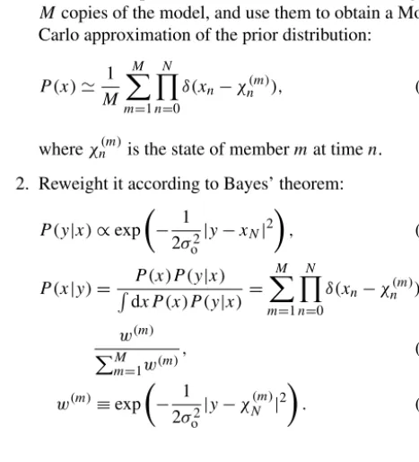
1. Generate samples of initial and model errors, integrate

Mcopies of the model, and use them to obtain a Monte Carlo approximation of the prior distribution:

P (x)' 1

M M X

m=1 N Y

n=0

δ(xn−χ_n(m)), (50)

whereχn(m)is the state of membermat timen.

2. Reweight it according to Bayes’ theorem:

P (y|x)∝exp

− 1 2σ2

o

|y−xN|2

, (51)

P (x|y)=_R P (x)P (y|x) dxP (x)P (y|x)=

M X

m=1 N Y

n=0

δ(xn−χ_n(m))

w(m)

PM

m=1w(m)

, (52)

w(m)≡exp

− 1 2σ2

o

|y−χ_N(m)|2

. (53)

3 Results

3.1 Example A (hyperbolic model)

In our first example, we solve the non-linear smoothing prob-lem for the hyperbolic model (Daum, 1986), which is a sim-ple problem with one-dimensional state space, but which has a non-linear drift term. We want to find the probability distri-bution of the paths described by

dxt =tanh(xt)dt+dwt, xt=0∼N(0,0.16), (54)

subject to an observationy:

y|xt=5∼N(xt=5,0.16), y=1.5. (55) The setting follows Daum (1986). In this case, divf (x)= 1/cosh2(x) imposes a penalty for small x. The total time durationT =5 is divided intoN=100 segments withδt=

5×10−2.

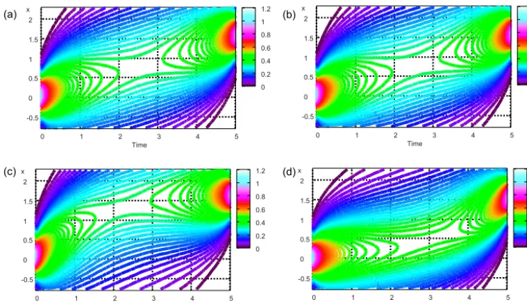
Figure 1 shows the probability densities of paths nor-malised on each time slice,Pt=n(φ)=

R

P (Uφ|y)dφt6=n,

de-rived by MCMC and PS. PS is performed with 5.1×1010 particles. It is clear that MCMC with E or TD provides the proper distribution matched with that of PS; this is also clear from the expected paths yielded by these experiments, as shown in Fig. 2. These schemes correspond to candidates in Eqs. (38) and (39). The expected path by ED bends towards a largerx, which should be caused by an extra penalty for a largerx. The expected path by T bends towards a smallerx, which should be caused by the lack of a penalty for a larger

x.

The results of 4D-Var, which represents the MAP esti-mates, are shown in Fig. 3. ED and TD provide the proper MAP estimate. These schemes correspond to candidates in Eqs. (41) and (42). The expected paths by E and T bend to-wards a smallerφ, which should be caused by the lack of a penalty for a largerφ.

3.2 Example B (Rössler model)

In our second example, we solve the non-linear smoothing problem for the stochastic Rössler model (Rössler, 1976). We want to find the probability distribution of the paths described by



 

 

dx1 =(−x2−x3)dt+σdw1, dx2 =(x1+ax2)dt+σdw2, dx3 =(b+x1x3−cx3)dt+σdw3,

(56)

xt=0∼N(xb,0.04I ), (57)

subject to an observationy:

y|xt=0.4∼N(xt=0.4,0.04I ), (58) where (a, b, c)=(0.2,0.2,6), σ=2, xb= (2.0659834,−0.2977757,2.0526298)T, and y=

(2.5597086,0.5412736,0.6110939)T. In this case, divf (x)=x1+a−c imposes a penalty for large x1. The total time duration T =0.4 is divided into N=800 segments withδt=5×10−4.

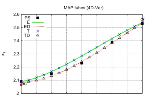
The results by MCMC and 4D-Var for the Rössler model are shown in Figs. 4 and 5, respectively. The state vari-able x1 is chosen for the vertical axes. PS is performed with 3×1012particles. The curve for PS in Fig. 5 indicates

ˆ

φ=argmax_φP (φ|y), whereUrepresents the tube centred at

0 1 2 3 4 5 Time

x

0 0.2 0.4 0.6 0.8 1 1.2

-0.5 0 0.5 1 1.5 2 x

0 1 2 3 4 5 -0.5

0 0.5 1 1.5 2

Time

x x

0 1 2 3 4 5 -0.5

0 0.5 1 1.5 2

Time

x

0 0.2 0.4 0.6 0.8 1 1.2 x

0 1 2 3 4 5 -0.5

0 0.5 1 1.5 2

Time

x

0 0.2 0.4 0.6 0.8 1 1.2 x

(a) (b)

(c) (d)

0 0.2 0.4 0.6 0.8 1 1.2

Figure 1.Probability density of paths derived by MCMC and PS for the hyperbolic model.(a)Reference solution by PS,(b)solution by MCMC with scheme E or TD,(c)solution by MCMC with scheme ED, and(d)solution by MCMC with scheme T.

-0.5 0 0.5 1 1.5 2

0 1 2 3 4 5

x

t

Mean orbits (MCMC)

BG

OBS

PS E ED T TD

Figure 2.Expected path derived by MCMC (hyperbolic model).

Figure 4 shows that, just as for the hyperbolic model, E and TD provide the proper expected path. Figure 5 shows that ED and TD provide the proper MAP estimate.

3.3 Towards application to large systems

When one computes the cost value J (x), the negative log-arithm of the posterior probability, in data assimilation, the value f (x) is explicitly computed by the numerical model while divf (x)is not. If the dimensionDof the state space is large, and f is complicated, the algebraic expression of divf (x)can be difficult to obtain. The gradient of the cost function∇J (x)contains the derivative of f (x), which can be implemented as the adjoint model by symbolic

differenti--0.5 0 0.5 1 1.5 2

0 1 2 3 4 5

x

t

MAP tubes (4D-Var)

BG

OBS

PS E ED T TD

Figure 3. Most probable tube derived by 4D-Var (hyperbolic model).

Table 1.Applicable OM schemes.

with div(f ) without div(f )

Sampling by MCMC Euler scheme X

trapezoidal scheme X MAP estimate by 4D-Var Euler scheme X trapezoidal scheme X

2 2.1 2.2 2.3 2.4 2.5 2.6

0 0.05 0.1 0.15 0.2 0.25 0.3 0.35 0.4

x1

t

Mean orbits (MCMC)

BG

OBS

PS E ED T TD

Figure 4.Expected path derived by MCMC (Rössler model).

2 2.1 2.2 2.3 2.4 2.5 2.6

0 0.05 0.1 0.15 0.2 0.25 0.3 0.35 0.4

x1

t MAP tubes (4D-Var)

BG

OBS

PS E ED T TD

Figure 5.Most probable tube derived by 4D-Var (Rössler model).

4 Conclusions

We examined several discretisation schemes of the OM functional, 1

2σ2

dx dt −f (x)

2

+1

2div(f ), for the non-linear smoothing problem

dxt =f (xt)dt+σdwt,

x0∼N(xb, σb2I ), (∀m∈M) ym|xm∼N(xm, σo2I ), by matching the answers given by MCMC and 4D-Var with that given by PS, taking the hyperbolic model and the Rössler

model as examples. Table 1 lists the discretisation schemes which were found to be applicable, i.e. those expected to con-verge to the same result as the reference solution. These re-sults are consistent with the literature (e.g. Apte et al., 2007; Malsom and Pinski, 2016; Dutra et al., 2014; Stuart et al., 2004).

This justifies, for instance, the use of the following cost function for the MAP estimate given by 4D-Var:

J=|φ0−xb| 2

2σ_b2 + X

m∈M

|φm−ym|2

2σ2 o

+δt N X

n=1 1 2σ2

φn−φn−1

δt −f (φn−1)

2 +1

2divf (φn−1)

!

,

wherenis the time index,δt is the time increment,xbis the background value,σb is the standard deviation of the back-ground value,y is the observational data,σois the standard deviation of the observational data, andσ is the noise inten-sity. However, the divergence term above should be excluded for the assignment of path probability in MCMC.

For application in large systems, the Euler scheme without the divergence term is preferred for path sampling because it does not require cumbersome calculation of the divergence term. In 4D-Var, the divergence term can be incorporated into the cost function by utilising Hutchinson’s trace estimator.

Code availability. The code for data assimilation is available at

Appendix A: Scaling of the terms

Taylor expansion of the f (ψn−1) term around ψ_n−1 2

in scheme E gives

g

OM'

N X

n=1 δt

σ−2

_ψn−ψn

−1 δt

−f (ψ_n−1 2)

−(ψn−ψn−1)

∂f ∂x(ψn−12)

2

+div(f ) )

=δt n

σ−2(noise+shift)2+divergenceo.

noise≡ψn−ψn−1

δt −f (ψn−12),

shift≡(ψn−ψn−1) ∂f

∂x(ψn−12),divergence

≡div(f ),

where we assume order-one fluctuations,σ =O(1),and the symbolψ represents eitherφfor a smooth curve orx for a sample path.

For a sample path of the stochastic process, the scaling is

ψn−ψn−1=O(δ

1 2

t ), which leads to

g

OM=Xδt 

 

 

σ−2 

 noise

2

| {z } δ_t−1

+noise×shift

| {z }

1

+shift2

| {z } δt



 

+divergence

| {z }

1







. (A1)

The shift term induces a Jacobian that coincides with the di-vergence term in TD (Zinn-Justin, 2002).

In the case of a smooth curve, there is no stochastic term, and thus ψn−ψn−1 is the product of a bounded function f (ψn−1)andδt, which results in a value withO(δt). This

leads to

g

OM=Xδt 

 

 

σ−2 

 noise

2

| {z }

1

+noise×shift

| {z }

δt

+shift2

| {z } δ2

t 

 

+divergence

| {z }

1







. (A2)

The shift term is negligible, but the divergence term is not.

Appendix B: Divergence term

B1 Divergence term in a trapezoidal scheme

Consider two stochastic processes (cf. Sect. 6.3.2 of Law et al., 2015):

dxt =f (xt)dt+dwt, x(0)=x0, (B1)

dxt=dwt, x(0)=x0, (B2)

where Eq. (B1) has measure µ and Eq. (B2) has measure

µ0(Wiener measure). By the Girsanov theorem, the Radon– Nikodym derivative ofµwith respect toµ0is

dµ

dµ0 =exp



−

T Z

0

₁

2|f (x)|

2_{dt−f (x)·dx}



. (B3)

If we define F (xT)−F (x0)=R_xxT₀ f (x)◦dx with the Stratonovich integral, then by Ito’s formula,

dF =f·dx+1

2div(f )dt. (B4)

Eliminatingf·dxin Eq. (B3) using Eq. (B4), we obtain

dµ

dµ0 =exp



−

T Z

0 1 2|f (x)|

2_{dt+F (x}

T)−F (x0)

−1 2

T Z

0

div(f )dt 

. (B5)

SubstitutingF (xT)−F (x0)=R₀Tf◦d_dx_tdt,

dµ

dµ0 =exp



−

T Z

0 1 2|f (x)|

2_dt+ T Z

0 f◦dx

dtdt

−1 2

T Z

0

div(f )dt 

. (B6)

If we write the Wiener measure formally as µ0(dx)= exp

−1 2

RT 0

dx dt

2 dt

dx,we get the following from Eq. (B3),

µ(dx)=exp



−

T Z

0 1 2

dx

dt −f (x)

2 dt



dx, (B7)

and the following from Eq. (B6),

µ(dx)=exp 

− T Z

0 1 2

dx dt −f (x)

2

+div(f ) !

dt 

dx, (B8)

where the integrals should be interpreted in the Ito sense and in the Stratonovich sense, respectively.

B2 Divergence term for smooth tube

Letxbe a diffusion process that follows the stochastic dif-ferential equation

dxt =f (xt)dt+dwt, (B9)

where w is a Wiener process. To investigate paths near a smooth curveφ, let us consider the following stochastic pro-cessxt−φ (t )(Ikeda and Watanabe, 1981; Zeitouni, 1989): d(xt−φ (t ))=(f (xt−φ (t )+φ (t ))− ˙φ (t ))dt+dwt. (B10) This means that if a driftf is applied to the Wiener process, and the reference frame is shifted byφ, the processxt−φ (t )

which has the driftf (· +φ)− ˙φis obtained. The weight rel-ative to the Wiener measure can be calculated by Girsanov’s formula as follows.

I(φ)≡

P (kx−φk_T < ) P (kwk_T < )

=_E  exp   T Z 0

f (wt+φ (t ))− ˙φ (t )

·dwt−

1 2 T Z 0

f (wt+φ (t ))− ˙φ (t ) 2 dt  

kwkT < i

, (B11)

where the expectation is taken with respect to the Wiener processwconditioned tokwk_T ≡sup0<t <T|wt|< .We are

going to evaluate the terms containingwtin the exponent on the RHS of Eq. (B11).

1. If we assumeφ is a twice continuously differentiable function, then by applying Ito’s product rule toφ (t )˙ ·wt, and using(∀t )|wt|< ,

T Z 0 ˙

φ (t )·dwt = ˙

φ (T )·wT−

T Z

0

wt· ¨φ (t )dt

≤A1, (B12)

whereA1is a positive constant independent of. 2. If we assumef is a twice continuously differentiable

function, then by using(∀t )|wt|< ,

T Z 0

f (wt+φ (t ))· ˙φ (t )dt−

T Z

0

f (φ (t ))· ˙φ (t )dt

≤A2, (B13)

whereA2is a positive constant independent of. 3. In the similar manner as in 1,

T Z 0

|f (wt+φ (t ))|2dt−

T Z

0

|f (φ (t ))|2dt

≤A3, (B14)

whereA3is a positive constant independent of.

4. The evaluation ofR₀Tf (wt+φ (t ))·dwt is as follows. a. By applying Taylor’s expansion tof (wt+φ (t )),

T Z

0

f (wt+φ (t ))·dwt= T Z

0

f (φ (t ))·dwt

+

T Z

0

(wt· ∇)f (φ (t ))·dwt+

T Z

0

O(w2)·dwt. (B15)

b. By applying Ito’s product rule towt·f (φ (t )), and

using(∀t )|wt|< , T

Z

0

f (φ (t ))·dwt=wT·f (φ (T ))

− T Z 0 X i,j wi_t∂fi

∂xj

(φ (t ))φj(t )˙ dt=O(). (B16)

c. Regarding the second term on the RHS of Eq. (B15), we see that

T Z

0

(wt· ∇)f (φ (t ))·dwt+1 2

T Z

0

∇ ·f (φ (t ))dt

= T Z 0 X i,j ∂fi ∂xj

(φ (t ))wj_tdw_ti+1 2 T Z 0 X i,j δij ∂fi ∂xj

(φ (t ))dt

= T Z 0 X i,j ∂fi ∂xj(φ (t ))

wj_tdwi_t+1 2δijdt

= T Z 0 X i,j ∂fi

∂xj(φ (t ))dζ j i

t , (B17)

whereζ_tj i=Rt 0w

j

s ◦dwis(Stratonovich integral).

By applying evaluations (1)–(4) to Eq. (B11), we obtain

I(φ)=exp  − 1 2 T Z 0

f (φ (t ))− ˙φ (t ) 2

dt−1

2 T Z

0

∇ ·f (φ (t ))dt   ×_E  exp 

O()+O(2)+ T Z 0 X i,j ∂fj ∂xi(φ (t ))dζ

j i t + T Z 0

O(|w|2)·dwt 



kwkT < 

. (B18)

On pages 450–451 in Ikeda and Watanabe (1981), it is shown that E  exp  c T Z 0 X i,j ∂fj ∂xi(φ (t ))dζ

j i t  

kwkT< 

 →0

−−→1 (∀c),

E 

exp 

c T Z

0

O(|w|2)·dwt 



kwkT < 

 →0

−−→1 (∀c),

(B20) and it is obvious that

E

h

expcO()+cO(2)

kwkT < i →0

−−→1 (∀c). (B21) They also showed that if

E h

exp caj

kwkT < i _→0

−−→1 (∀c) (B22)

forj=1,2,· · ·, J, then

E "

exp

J X

j=1 aj

!

kwkT < #

→0

−−→1. (B23)

By applying this to Eqs. (B20), (B19), and (B21), we deduce from Eq. (B18) that

I(φ) →0 −−→

exp 

− 1 2

T Z

0

f (φ (t ))− ˙φ (t ) 2

dt−1

2 T Z

0

∇ ·f (φ (t ))dt 

. (B24)

From evaluation (4), we also have that

E 

exp 

 T Z

0

f (wt+φ (t ))·dwt 



kwkT < 



→0 −−→exp



−

1 2

T Z

0

divf (φ (t ))dt 

. (B25)

Equation (B25) serves as an evaluation formula for the di-vergence term along φby ensemble calculation if we inter-pret the expectation as an ensemble average:

lnE 

exp 

 T Z

0

f (wt+φ (t ))·dwt 



kwkT < 

 →0 −−→

−1 2

T Z

0

divf (φ (t ))dt. (B26)

The ensemble can be generated by using a Wiener process limited to the small areakwk_T < . Taking the derivative of Eq. (B26) with respect toφi(t ), we also obtain the formula

for evaluating the derivative of the divergence term alongφ, as follows.

E h

∇f (φ+w)·dwexpR₀Tf (φ+w)·dw

kwkT < i

E h

expR₀Tf (φ+w)·dw

kwkT < i

→0 −−→ −1

2∇(divf )dt, (B27)

where (∇f (φ+w),dw)=P j

∂fj(φ+w)

∂φi dwj can be

calcu-lated using the adjoint model ∇f (φ+w). Although these evaluation formulas (B26) and (B27) illustrate the meaning of the divergence term, they seem too expensive to be used in the 4D-Var iterations.

Appendix C: Estimator for the divergence term

Cost functions in Eqs. (42) and (41) utilise the derivative of the drift termf (x), and thus the gradient of the term con-tains the second derivative off (x), whose algebraic form is difficult to obtain in high-dimensional systems. Here, we pro-pose an alternative form using Hutchinson’s trace estimator (Hutchinson, 1990), which approximates the trace of matrix

E[ξTAξ] =tr(A) using a stochastic vector whose

compo-nents are independent, identically distributed stochastic vari-ables that take value±1 with probability 0.5.

A realisation of the cost function is given as ˆ

Jtube(φ|y)= 1 2σ_b2

|φ0−xb|2+

X

m∈M

1 2σ2

o

|φm−ym|2

+δt N X

n=1 1 2σ2

φn−φn−1

δt −f (φn−1)

2

+1 2ξ

T n−1b

−1

f (φn−1+bξn−1)−f (φn−1)

, (C1)

wherebis a small number. Note thatJˆtube(φ|y)is a stochastic variable that satisfies

E h

ˆ

Jtube(φ|y)

i

=Jtube(φ|y). (C2) If the adjoint off is at hand, the gradient of the stochastic cost function is given as

∇_φnJˆtube(φ|y)= 1

σ_b2(φ0−xb)δ0,n+ X

m∈M

1

σ2 o

(φm−ym)δm,n

+ 1

σ2

φn−φn−1

δt −f (φn−1)

(n >0)

+ δt

σ2 − 1

δt

−

_∂f

∂φn (φn)

T!_φ

n+1−φn δt

−f (φn)

(n < N )

+δt 2

"

∂f ∂φn

(φn+bξn) T

b−1ξn−

∂f ∂φn

(φn) T

b−1ξn #

.

(n < N ) (C3)

Competing interests. The author declares that she has no conflict of interest.

Acknowledgements. The author is grateful to the referees for their

comments which helped improve the readability of the paper. This work was partly supported by MEXT KAKENHI Grant-in-Aid for Scientific Research on Innovative Areas JP15H05819. All the numerical simulations were performed on the JAMSTEC SC supercomputer system.

Edited by: Zoltan Toth

Reviewed by: two anonymous referees

References

Apte, A., Hairer, M., Stuart, A. M., and Voss, J.: Sampling the pos-terior: An approach to non-Gaussian data assimilation, Phys. D, 230, 50–64, https://doi.org/10.1016/j.physd.2006.06.009, 2007. Cotter, S. L., Roberts, G. O., Stuart, A., and White, D.: MCMC

methods for functions: modifying old algorithms to make them faster, Stat. Sci., 28, 424–446, 2013.

Daum, F.: Exact finite-dimensional nonlinear filters, IEEE T. Au-tomat. Contr., 31, 616–622, 1986.

Doucet, A., Godsill, S., and Andrieu, C.: On sequential Monte Carlo sampling methods for Bayesian filtering, Stat. Comput., 10, 197– 208, 2000.

Dutra, D. A., Teixeira, B. O. S., and Aguirre, L. A.: Maximum a posteriori state path estimation: Discretization limits and their interpretation, Automatica, 50, 1360–1368, 2014.

Giering, R. and Kaminski, T.: Recipes for adjoint code construction, ACM Transactions on Mathematical Software (TOMS), 24, 437– 474, 1998.

Hutchinson, M. F.: A stochastic estimator of the trace of the in-fluence matrix for laplacian smoothing splines, Commun. Stat. Simulat., 19, 433–450, 1990.

Ikeda, N. and Watanabe, S.: Stochastic Differential Equations and Diffusion Processes, vol. 24 of North-Holland Mathematical Li-brary, chap. VI.9, North-Holland, 1981.

Law, K., Stuart, A., and Zygalakis, K.: Data Assimilation, Springer, 2015.

Malsom, P. J. and Pinski, F. J.: Role of Ito’s lemma in sampling pinned diffusion paths in the continuous-time limit, Phys. Rev. E, 94, 042131, https://doi.org/10.1103/PhysRevE.94.042131, 2016. Metropolis, N., Rosenbluth, A. W., Rosenbluth, M. N., Teller, A. H., and Teller, E.: Equation of state calculations by fast computing machines, J. Chem. Phys., 21, 1087–1092, 1953.

Onsager, L. and Machlup, S.: Fluctuations and ir-reversible processes, Phys. Rev., 91, 1505, https://doi.org/10.1103/PhysRev.91.1505, 1953.

Roberts, G. O. and Rosenthal, J. S.: Optimal scaling of discrete ap-proximations to Langevin diffusions, J. R. Stat. Soc. B, 60, 255– 268, 1998.

Rössler, O.: An equation for continuous chaos, Phys. Lett. A, 57, 397–398, https://doi.org/10.1016/0375-9601(76)90101-8, 1976. Stuart, A. M., Voss, J., and Wilberg, P.: Conditional Path Sampling

of SDEs and the Langevin MCMC Method, Commun. Math. Sci., 2, 685–697, 2004.

Trémolet, Y.: Accounting for an imperfect model in 4D-Var, Q. J. Roy. Meteor. Soc., 132, 2483–2504, https://doi.org/10.1256/qj.05.224, 2006.

Zeitouni, O.: On the Onsager–Machlup functional of diffusion pro-cesses around non C2 curves, Ann. Probab., 17, 1037–1054, 1989.

Zinn-Justin, J.: Quantum Field Theory and Critical Phenomena, chap. 4.6, Oxford University Press, 4th Edn., 2002.