www.ocean-sci.net/8/19/2012/ doi:10.5194/os-8-19-2012
© Author(s) 2012. CC Attribution 3.0 License.
Ocean Science
The vertical structure of oceanic Rossby waves: a comparison of
high-resolution model data to theoretical vertical structures
F. K. Hunt1, R. Tailleux2, and J. J.-M. Hirschi3
1Ocean and Earth Science, National Oceanography Centre Southampton, University of Southampton, Southampton, UK
2Department of Meteorology, University of Reading, Reading, UK 3National Oceanography Centre, Southampton, UK
Correspondence to: F. K. Hunt ([email protected])
Received: 20 April 2011 – Published in Ocean Sci. Discuss.: 13 May 2011
Revised: 30 September 2011 – Accepted: 12 December 2011 – Published: 13 January 2012
Abstract. Tests of the new Rossby wave theories that have been developed over the past decade to account for discrep-ancies between theoretical wave speeds and those observed by satellite altimeters have focused primarily on the surface signature of such waves. It appears, however, that the surface signature of the waves acts only as a rather weak constraint, and that information on the vertical structure of the waves is required to better discriminate between competing theories.
Due to the lack of 3-D observations, this paper uses high-resolution model data to construct realistic vertical structures of Rossby waves and compares these to structures predicted by theory. The meridional velocity of a section at 24◦S in the Atlantic Ocean is pre-processed using the Radon transform to select the dominant westward signal. Normalized profiles are then constructed using three complementary methods based respectively on: (1) averaging vertical profiles of velocity, (2) diagnosing the amplitude of the Radon transform of the westward propagating signal at different depths, and (3) EOF analysis. These profiles are compared to profiles calculated using four different Rossby wave theories: standard linear theory (SLT), SLT plus mean flow, SLT plus topographic fects, and theory including mean flow and topographic ef-fects. Our results support the classical theoretical assump-tion that westward propagating signals have a well-defined vertical modal structure associated with a phase speed inde-pendent of depth, in contrast with the conclusions of a recent study using the same model but for different locations in the North Atlantic. The model structures are in general surface intensified, with a sign reversal at depth in some regions,
no-tably occurring at shallower depths in the East Atlantic. SLT provides a good fit to the model structures in the top 300 m, but grossly overestimates the sign reversal at depth. The ad-dition of mean flow slightly improves the latter issue, but is too surface intensified. SLT plus topography rectifies the overestimation of the sign reversal, but overestimates the am-plitude of the structure for much of the layer above the sign reversal. Combining the effects of mean flow and topog-raphy provided the best fit for the mean model profiles, al-though small errors at the surface and mid-depths are carried over from the individual effects of mean flow and topogra-phy respectively. Across the section the best fitting theory varies between SLT plus topography and topography with mean flow, with, in general, SLT plus topography performing better in the east where the sign reversal is less pronounced. None of the theories could accurately reproduce the deeper sign reversals in the west. All theories performed badly at the boundaries. The generalization of this method to other lati-tudes, oceans, models and baroclinic modes would provide greater insight into the variability in the ocean, while bet-ter observational data would allow verification of the model findings.
1 Introduction
Rossby wave issue that was prompted by the pioneering study by Chelton and Schlax (1996). However, the nature of satellite observations also means that improved theories of Rossby wave propagation have focused so far only on the surface signature of such waves, with little being known on how such theories would perform on the predictions of the vertical structure of such waves for lack of suitable ob-servations. Thus, Tailleux and McWilliams (2001) showed how two physically different theories for Rossby waves, one based on the bottom-pressure compensated theory (which in effect accounts for the effect of rough bottom topography but no background mean flow) and that of the mean flow theory of Killworth et al. (1997) in a flat bottom ocean both were able to reproduce observed phase speeds with approximately the same degree of scatter while being based on fundamen-tally different physical principles. As shown in the present paper, these two theories however predict significantly differ-ent vertical structures for the Rossby waves, suggesting that insights into the actual vertical structure of observed Rossby waves may help in discriminating between different theories. Rossby waves play a critical role in the climate system, acting as a large scale adjustment mechanism for ocean basins to buoyancy forcing (Pedlosky, 1979; Gill, 1982), in-fluencing the intensification (Anderson and Gill, 1975; An-derson and Killworth, 1977; Deser et al., 1999) and position (Taguchi et al., 2005) of western boundary currents and pro-viding a possible source of variability in the Atlantic Merid-ional Overturning Circulation (Hirschi et al., 2007). Rossby waves are also associated with quasi-periodic climate cy-cles, such as the El Ni˜no-Southern Oscillation (Picaut et al., 1997).
The interaction of the displacement of density gradients and the transport of energy by Rossby waves is important in all these processes; however, the understanding of these vi-tal oceanic and climatic phenomena is hindered by a lack of knowledge of the vertical structure of Rossby waves. These density adjustments provide a link in the feedback between the atmospheric forcing of the ocean and the oceanic forc-ing of the atmosphere, but their slow speed delays the trans-mission of these forcings between ocean regions by years to decades. This can potentially be exploited to predict the seasonal to decadal behaviour of the system, but requires more than a surface understanding. While the vertical struc-ture is unknown the reliability of the results of seasonal and longer-term climate models remains uncertain because their representation of the full structure of Rossby waves cannot be validated. Additionally, Rossby wave characteristics may change with a changing climate (Fyfe and Saenko, 2007), the effects and feedbacks of which cannot be fully appreciated from a surface-only perspective.
Typical investigations of Rossby waves based on linear theory decompose the wave into an infinite number of verti-cal “normal modes”, and their analogous forms in WKB the-ory, and assume that the phase speed is independent of depth. This produces vertical waveforms such as the barotropic
mode and the first and second baroclinic modes. Com-monly observations of Rossby waves are interpreted as the first baroclinic mode, prompting a search for factors that could increase the speed of this mode to match the enhanced speeds calculated from satellite observations (Killworth et al., 1997); however, as noted by Tailleux (2003), topogra-phy may slow down the barotropic mode enough as to make its phase speed close to observed ones. The assumption that distinct modes of propagation still persist in the presence of a nonzero background mean flow, topography, nonlinearities, and diabatic processes, and that these are characterized by a vertically-coherent structure with a well-identified propaga-tion speed independent of depth has been widespread so far, but still remain to be fully validated for lack of suitable obser-vational data, although some attempts at doing so have been recently developed as reviewed below.
Previous sub-surface or in-situ observations of Rossby waves have often been restricted to a single, or a few, depth levels and thus limited in their ability to resolve the full 3-D structure. However recent hydrographic measurements have been able to provide some insight. For example, in Hagen (2005), transects of the top 1000 m of the Northeast Atlantic were shown to exhibit significant undulations in po-tential density surfaces, decreasing in amplitude with depth to become almost insignificant below 250 dbar at 10◦N and below 500 dbar at 21◦N, suggesting surface intensification. Vertical structures found by decomposition of the data into eigenfunctions yielded surface intensification of the waves that was more prominent the further north the section and which reduced in magnitude with depth, slightly increasing in speed at the ocean bottom and showing no reversal of ve-locity in the profile, contrary to the expectations from stan-dard linear theory for the first baroclinic mode.
ARGO profiling floats provide a hope of a widespread method for detecting the structure of Rossby waves below the surface. Chu et al. (2007) used data from ARGO floats in the North Atlantic to extract vertical profiles of Rossby waves. They found that the second baroclinic mode was al-ways dominant, with the contributions of other modes ge-ographically variable. This produced profiles with a sub-surface maximum at approximately 1000 m and a secondary maximum in the region of 100 m with no reversal at depth, in concurrence with the results of Hagen (2005). Overall these studies support Chelton and Schlax (1996)’s conclusions that the standard linear theory for Rossby waves is inadequate to account for the properties of actual signals.
in a high-resolution z-coordinate model on selected isopy-cnal surfaces in the North-Atlantic Ocean and found a sys-tematic slow down of the simulated waves with depth, in contrast with the assumption made in most Rossby wave theories that Rossby waves propagate as vertically-coherent structures with a phase speed independent of depth. A com-parison of theoretical profiles of meridional velocity to those generated by a high resolution model of the Pacific by Aoki et al. (2009) found a surface intensified wave from the model data that was comparable to theoretical vertical structures that included the effects of mean flow and topography. Fur-thermore they found the fit improved with the addition of finite wavelength effects.
In the present study, we seek to develop further insights into the issue by using 3 different methods to generate em-pirical vertical structures of Rossby wave propagation in the Atlantic Ocean using velocity anomalies from the same high-resolution numerical model as used in Lecointre et al. (2008). Unlike in the latter study, however, the velocity anomalies are not projected on isopycnal surfaces, but retained in their orig-inal z-coordinate system. Moreover, we then seek to com-pare the empirical vertical structures obtained with those pre-dicted by the standard and extended Rossby wave theories, similarly as in Aoki et al. (2009), to evaluate their success, and determine whether the performances of any given theory extend to the whole water column.
Section 2 describes how vertical structures are constructed from the model data and how the theoretical structures are determined. Section 3 presents the structures identified and compares them to theory, while Sect. 4 discusses the results and their context. Section 5 draws conclusions from the study and gives recommendations for further research.
2 Method
This model’s ability to produce realistic simulations of oceanic Rossby waves has been tested with observed and simulated surface phase speeds and shows good agreement (Lecointre et al., 2008). The model also performs well in a comparison between observed and simulated eddy kinetic energy (Penduff et al., 2004), which is important considering the possibility of interpreting the westward propagating sig-nals as eddies rather than waves (Chelton et al., 2007). The good agreement between observed and simulated character-istics of baroclinic wave and eddy activities in the sea surface height suggest that it is reasonable to assume that the degree of realism achieved for the surface signature of the variabil-ity also pertain to its vertical structure, which motivates the use of such a model for the present study.
The method and technique developed in this study to in-vestigate the vertical structure of westward propagating sig-nals is illustrated for a particular longitudinal section. Specif-ically, a section at 24◦S is chosen for investigation due to strong Rossby wave propagation in this region and the range
42
1
2
Figure 1. Bottom topography of section at 24o S.
3
Longitude (degrees)
Depth (m)
−40 −30 −20 −10 0 10
0 1000 2000 3000 4000 5000
Fig. 1. Bottom topography of section at 24◦S.
of bottom topography at this location, including the conti-nental slope, which is relatively gentle; the abyssal plane, which is flat; the Mid-Atlantic Ridge, which has some sharp topography; and the Walvis Ridge, which forms a very sharp topographic barrier in the east (see Fig. 1 for section topog-raphy). This allows the influence of bottom topography on the vertical structures to be evaluated in different conditions. In order to investigate the possible importance of the par-ticular methodology used, three different methods were used to construct empirical vertical structures from the meridional velocity component, respectively based on:
1. using the Radon-filtered meridional velocity; 2. using the amplitude of the Radon transform; 3. using empirical orthogonal functions (EOFs).
The underlying motivation for using these three different methods was to contrast the structures found using the more traditional and established method based on EOFs with sim-pler and more experimental methods involving less process-ing of the raw data. Their agreement (and disagreement) pro-vides insights into the nature of the data, as it is not known a priori what the “true” vertical structure should be. Indeed, even though one might expect the EOF-based method to be superior, it is important to note that there is no theoretical justification or mathematical proof that this should be neces-sarily the case. For instance, it is well known that the vertical modal structures of the generalized linear theory in presence of background mean flow and topography are not orthogonal for the natural inner-product serving to construct the EOFs.
speed. This procedure is repeated for all depth levels. For depth levels that intersect topography the longitudes occu-pied by the topography are set to zero and the Radon trans-form still applied to the entire section. This does not affect the result of the Radon transform as it is basically a summa-tive process and so not affected by additional zeros, however the proportion of the section occupied by water necessarily decreases with depth so the Radon transform is based on less data as the depth increases. It was occasionally found that the dominant speed at a particular level would differ from that exhibited by the surface level; in general, however, the Radon power would nevertheless exhibit a secondary peak corre-sponding to the dominant surface speed, in which case the Gaussian filter would therefore be applied to the secondary peak, rather than to the dominant peak, in order to isolate a vertical Rossby wave structure associated with vertically co-herent propagation, as is usually assumed in WKB theories of Rossby wave propagation. This procedure was repeated for two sub-domains representing the east and west Atlantic basins, spanning−37.75◦to−16.42◦, down to 4000 m and
−9.91◦ to 4.42◦, down to 4200 m respectively, to find the dominant phase speed in each basin. The Radon analysis of the Western and Eastern Atlantic basins suggests that the dominant phase speed does not vary appreciably in longi-tude. This motivates the use of a Gaussian filter centred on a common phase speed and justifies carrying out the analysis over the full Atlantic basin. Moreover, as neither the western nor the eastern sections intercept topography while still lead-ing to a dominant phase speed similar to that obtained over the full section, the analysis suggests that our handling of the topography does not impact the results. Each of the meth-ods constructs profiles that are normalized by their absolute maximum to produce profiles that are easily comparable both between methods and with the theoretical profiles.
The first method constructs vertical profiles of meridional velocity from the back-transformed and filtered data at each time and longitude, which are each normalized by their ab-solute maximum. The profiles are then averaged over time to produce an average profile for each longitude (creating a meridional section of vertical structures), or averaged over time and longitude to produce a single average profile repre-sentative of the section. In general, the vertical structure ob-tained by averaging the normalized vertical structures does not necessarily vary between−1 and 1, and therefore has to be renormalized.
In order to illustrate the range of vertical structures spanned, the standard deviation (SD) of the individual nor-malized profiles is added to and subtracted from the mean profile. This provides a typical “envelope” of possible val-ues. As the focus is on the vertical structures, the standard deviation profiles are renormalized to bring their absolute maximum to unity, in order to make all profiles compara-ble. The resulting structures can be compared to the mean to discover how the structure might vary within the data. This process is repeated for each of the following methods.
In the second method, the vertical structures are estimated directly from the Gaussian-filtered Radon transform before it is back-transformed. Specifically, a vertical profile is con-structed from the amplitude of the filtered Radon transform at each depth of the model, which is then normalized, av-eraged and re-normalized as in the previous method. The standard deviation is also calculated and applied to the mean in the manner described above. This method yields a vertical profile pertaining to the entire longitudinal section that the Radon is applied to, and therefore does not vary with longi-tude by construction, unlike the other methods.
The third method uses empirical orthogonal functions (EOFs) to determine the structures in the back-transformed filtered velocity data, i.e. not on the full meridional velocity data, but only on the part of the meridional velocity anoma-lies associated with westward propagation at the dominant speed, as described above. EOF analysis is conducted on the time series at each longitude, using MATLAB’s SVD func-tion (for more informafunc-tion about EOFs and their calculafunc-tion see Hannachi et al., 2007). The structure represented by the first EOF accounts on average for 72 % of the variance in the data (maximum 91 % (over rough/sharp topography), mini-mum 58 % in the flatter regions), therefore the first EOF was taken to be the representative structure in the data. When the data is reconstructed using the first EOF there is a vertical structure defined for each location at each time and the data is then treated in the same way as the normalized velocity method by normalization, averaging and re-normalization. The standard deviation is again treated as above.
The Radon amplitude method is associated with the least data processing, as it is performed on the data before it is back-transformed, and the EOF analysis is associated with the most data processing. This makes it possible to see how each added level of processing affects the data, with similar-ities across the different methods bringing re-assurance that methodological aspects do not introduce biases (at least in any significant way) to the empirically determined vertical structures.
salinity fields to calculate profiles of buoyancy frequency squared (N2). The theoretical basis for these scenarios is presented below.
The Rossby wave theory is based on the quasi-geostrophic vorticity equation (see Pedlosky (1979) for derivation): ∂ ∂t− ∂ψ ∂y ∂ ∂x+ ∂ψ ∂x ∂ ∂y "
∇2ψ+βy+ ∂
∂z f2 N2 ∂ψ ∂x !#
=0 (1) where: t= time, x= eastward coordinate, y= northward coordinate, z= vertical coordinate, ψ= geostrophic stream function,f= Coriolis parameter,β=north/south gradient of f,N2= buoyancy frequency.
The influence of the background meridional velocity can be neglected due to its limited impact on the phase speed (Killworth et al., 1997), therefore the geostrophic stream function can be written as:ψ= −U (z)y+φ (x,y,z,t ), to de-scribe wave-like perturbations to the background flow. When the stream function is substituted into the above equation and linearized with respect to φ the result, from Aoki et al. (2009), is:
∂ ∂t+U
∂ ∂x
"
∇2φ+ ∂
∂z f2 N2 ∂φ ∂z !# + " β− ∂ ∂z f2 N2 ∂U ∂z !# ∂φ
∂x=0 (2)
The wave solution of the above equation is taken as φ=
8(z)exp[i(kx+ly−σ t )], where 8(z) is the amplitude, which yields:
(U−c) "
−K28+ d
dz f2 N2 d8 dz !# + " β− d
dz f2 N2 dU dz !#
8=0 (3)
where:c=σ
k andK
2=k2+l2.
The boundary conditions for this equation at the surface and the bottom determine the vertical structure and phase speed.
The standard linear theory (Rossby, 1939; Gill, 1982) as-sumes a rigid lid (i.e. the vertical velocity vanishes at the sur-face and bottom) and no mean flow with a flat bottom. These assumptions simplify Eq. (3) to give:
d dz f2 N2 d8 dz ! + −β
c−K 2
8=0 (4)
using boundary conditions of:w∝d8
dz =0 atz=0,−H.
This equation and boundary conditions can be used to de-termine the vertical structure of the wave through an eigen-value problem. There are an infinite number of vertical modes of increasing complexity, however the mode of inter-est here is the first baroclinic mode. This theory is referred to as the “no mean flow, flat bottom theory” denoted “SLT”.
If the effects of the mean flow on the meridional compo-nent of the local potential vorticity is included then the equa-tion becomes:
(U−c) " d dz f2 N2 d8 dz !# + " β− d
dz f2 N2 dU dz !#
8=0 (5)
with boundary conditions of:(U−c)d8dz−dU
dz8=0
atz=0,−H.
This theory is referred to as “mean flow, flat bottom the-ory” denoted “U-Flat” and is the type of problem investi-gated by Killworth et al. (1997).
Bottom pressure decoupling or compensation is a theory put forward by Tailleux and McWilliams (2001) to account for the influence of topography whereby the waves are sur-face intensified and nearly insensitive to the bottom. This theory gives a profile using the boundary conditionsφ=0 at z= −H with the above equation. This theory is the “mean flow, bottom pressure decoupling theory” denoted “U-BPD” and, withU=0, the “no mean flow, bottom pressure decou-pling theory” denoted “BPD”.
The model profiles are compared to the theoretical pro-files using the root mean square error (RMSE). The lower the RMSE value the smaller the error between the profiles and so the better the fit. The RMSE is calculated according to:
RMSE=
s P
(xt−xm)2
n (6)
where xt= theoretical profile, xm= model profile and n= number of points in the profile.
The correlation between the RMSE and different variables can help highlight possible causes of the errors between the model sections and theoretical sections. The variables com-pared to the section RMSEs are: the mean flow,U; the unfil-tered meridional velocities,v; the filtered meridional velocity anomalies; the buoyancy frequency,N2; and the topography. A correlation can either be positive (the RMSE increases as the value of the variable increases) or negative (the RMSE in-creases as the value of the variable dein-creases) and the closer to one the correlation coefficient (R) is the stronger the cor-relation. It is calculated using Eq. (7). The significance of the correlation is tested at the 99 % confidence level using a t-test.
R= n
P
xtxm− P xt P
xm r
h nP
xt2− P
xt2i hnP x2
m− P
xm2i
(7)
3 Results
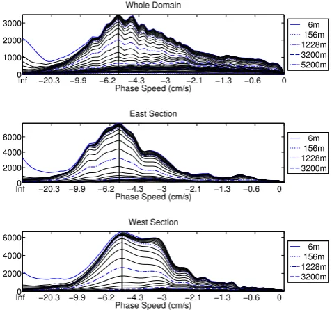
The amplitude of the Radon transform of the meridional ve-locity anomalies at 24◦S before filtering is shown in Fig. 2a at a number of selected depths; each line is normalized by its maximum so that the lines are on the same scale, as the am-plitude decreases with depth. Figure 3a shows the same data without normalization. The phase speed at which the am-plitude is maximum (corresponding to the signal selected by the filter) is indicated with a vertical black line and it is clear that while the maximum of every layer does not necessarily lie on this line, there is always at least a local maximum in the same location. This vertical coherence extends through-out the water column. This is the location chosen to apply the Gaussian filter and corresponds to selecting a wave speed of 5.6 cm s−1. Figure 3 clearly shows several other peaks in the Radon transform, these are excluded from the data by the filter. The second, third and fourth peaks for the whole do-main correspond to phase speeds of 4.8 cm s−1, 4.1 cm s−1 and 3.7 cm s−1respectively.
When split into East Atlantic and West Atlantic sections the same vertical coherence is seen; (see Figs. 2 and 3) with very similar phase speeds identified (shown by the vertical black lines), with the dominant phase speed in the east at 5.5 cm s−1and 5.3 cm s−1in the west. This justifies selecting a single phase speed to filter for the entire basin.
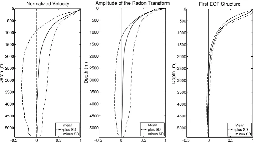
The means of the model profiles constructed using the three different methods, shown by the solid lines in Fig. 4, display some striking similarities as well as some differ-ences. The structure is consistently surface intensified, the Radon amplitude profile being most so, showing decreasing amplitude with depth, becoming zero, or near zero at the bot-tom. The EOF profile decreases most rapidly of the three below 1000 m, showing a very small sign reversal below about 2900 m, while the normalized velocity profile reaches zero amplitude around 4000 m, becoming briefly negative, whereas the Radon amplitude profile remains positive for the entire depth, only reaching zero at the bottom.
The envelope of the profiles obtained from the addition and subtraction of one standard deviation provides an insight into the variety of structures that make up the mean and are shown in Fig. 4 by the dashed lines. In all three cases they show that there are likely to be profiles in some locations that have a quite significant sign reversal occurring between 900 and 2000 m, although it is less pronounced in the EOF case. The normalized velocity and Radon amplitude +1 SD profiles indicate that there are also locations that see no sign reversal.
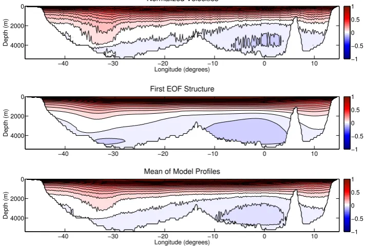
The longitudinal changes in structure obscured by the mean profiles are striking, as shown in Fig. 5. There is a significant deepening of the depth of sign reversal from east to west and eastwards of the Walvis Ridge, with the sign re-versal disappearing in places westwards of between 30 and 35◦W. The EOF section is significantly smoother than the normalized velocity section as the variance not explained by
Inf −20.3 −9.9 −6.2 −4.3 −3 −2.1 −1.3 −0.6 0 0
0.5 1
Phase Speed (cm/s) Whole Domain
6m 156m 1228m 3200m 5200m
Inf 0 −20.3 −9.9 −6.2 −4.3 −3 −2.1 −1.3 −0.6 0 0.5
1
Phase Speed (cm/s) East Section
6m 156m 1228m 3200m
Inf 0 −20.3 −9.9 −6.2 −4.3 −3 −2.1 −1.3 −0.6 0 0.5
1
Phase Speed (cm/s) West Section
6m 156m 1228m 3200m
Fig. 2. The normalized amplitude of the Radon transform with
phase speed for (a) the whole domain, (b) the East Atlantic and (c) the West Atlantic. Black vertical lines indicate the dominant phase speed.
Inf −20.3 −9.9 −6.2 −4.3 −3 −2.1 −1.3 −0.6 0 0
1000 2000 3000
Phase Speed (cm/s) Whole Domain
6m 156m 1228m 3200m 5200m
Inf 0 −20.3 −9.9 −6.2 −4.3 −3 −2.1 −1.3 −0.6 0 2000
4000 6000
Phase Speed (cm/s) East Section
6m 156m 1228m 3200m
Inf 0 −20.3 −9.9 −6.2 −4.3 −3 −2.1 −1.3 −0.6 0 2000
4000 6000
Phase Speed (cm/s) West Section
6m 156m 1228m 3200m
Fig. 3. The non-normalized amplitude of the Radon transform with
phase speed for (a) the whole domain, (b) the East Atlantic and (c) the West Atlantic. Black vertical lines indicate the dominant phase speed.
−0.5 0 0.5 1 0
500
1000
1500
2000
2500
3000
3500
4000
4500
5000
Normalized Velocity
Depth (m)
mean plus SD minus SD
−0.5 0 0.5 1
0
500
1000
1500
2000
2500
3000
3500
4000
4500
5000
Amplitude of the Radon Transform
Depth (m)
Mean plus SD minus SD
−0.5 0 0.5 1
0
500
1000
1500
2000
2500
3000
3500
4000
4500
5000
Depth (m)
First EOF Structure
Mean plus SD minus SD
Fig. 4. Normalized vertical profiles from the model data with their normalized±1 standard deviation (SD) profiles. (a) The normalized velocity method, (b) the amplitude of the Radon transform method and (c) the EOF method.
more rapidly with depth than is seen in the normalized velocity profiles. The average of these two sections is used for comparison with the theoretical sections and is shown in the bottom panel of Fig. 5.
The sections illustrate that the structures found by the ad-dition and subtraction of the standard deviation from the mean profile are representative of the range of structures in the section and so form a simple and succinct way to display the variability within the section.
The vertical profiles obtained from the four different theo-ries and their standard deviations, are shown in Fig. 6 along-side those profiles obtained from the model data. The SLT shows a steady decrease in amplitude with depth resulting in a sign reversal at between 1000 and 1500 m, and remains negative throughout the water column, even for the structures taking account of the SD, albeit with a very small shift to-wards zero with depth although values remain significantly negative at the bottom. TheU-Flat profile is more surface in-tensified than the SLT profile, with the amplitude decreasing quickly in the surface layer, slowing to a more gradual reduc-tion below around 200 m. A sign reversal occurs for all three structures between 1000 and 1400 m and maintains a more or less constant negative value with depth, although the plus SD structure remains much closer to zero, while the minus SD structure reaches negative values similar to those in the SLT profiles. This theory shows the biggest range of structures within the data. The BPD structures display a slow but steady decease in amplitude with depth, not reaching zero until af-ter 2500 m, which is considerably deeper than the SLT and
U-Flat profiles, after which both the mean and SD structures remain extremely close to zero. TheU-BPD profiles show a very similar rapid surface decline to that seen in theU-Flat structures, although the following slow down in rate of de-cline is greater in this case, being more characteristic of the BPD structures, again not reaching zero until after 2500 m and continuing very close to zero for the remaining depth.
Longitude (degrees)
Depth (m)
Normalized Velocities
−40 −30 −20 −10 0 10
0
2000
4000
−1 −0.5 0 0.5 1
Depth (m)
First EOF Structure
−40 −30 −20 −10 0 10
0
2000
4000
−1 −0.5 0 0.5 1
Longitude (degrees)
Depth (m)
Mean of Model Profiles
−40 −30 −20 −10 0 10
0
2000
4000
−1 −0.5 0 0.5 1
Fig. 5. Longitudinal sections showing the model profiles. (a) The normalized velocity method, (b) the EOF method, and (c) the mean of (a)
and (b) i.e. the mean model section. Contour interval is 0.05.
−0.5 0 0.5 1
0
500
1000
1500
2000
2500
3000
3500
4000
4500
5000
Depth (m)
SLT
mean plus SD minus SD Normalized V Radon Amplitude EOF
−0.5 0 0.5 1
0
500
1000
1500
2000
2500
3000
3500
4000
4500
5000
Depth (m)
U flat
mean plus SD minus SD Normalized V Radon Amplitude EOF
−0.5 0 0.5 1
0
500
1000
1500
2000
2500
3000
3500
4000
4500
5000
Depth (m)
BPD
mean plus SD minus SD Normalized V Radon Amplitude EOF
−0.5 0 0.5 1 0
500
1000
1500
2000
2500
3000
3500
4000
4500
5000
Depth (m)
U BPD
mean plus SD minus SD Normalized V Radon Amplitude EOF
Fig. 6. Theoretical vertical profiles with their normalized±1 standard deviation (SD) profiles (black curves). (a) Standard linear theory, (b) mean flow with a flat bottom, (c) no mean flow with topography and (d) mean flow and topography. The grey lines are the same in each panel and show the model profiles for the 3 methods as a comparison.
The decrease from the surface is too slow and steady in the BPD profile and consequently the fit above about 1700 m is poor, however the fit below this depth is very good, although it does not permit the sign reversals seen in the model pro-files however small. TheU-BPD profiles agree much more closely with the model profiles, although the decrease is too rapid in the top few hundred meters then too slow down to
1500 m, however the discrepancies are not very large, while the agreement is excellent at depth.
−0.5 0 0.5 1 0
500
1000
1500
2000
2500
3000
3500
4000
4500
5000
Mean Model Profiles
Depth (m)
Mean Model Normalized V Radon Amplitude EOF
−0.5 0 0.5 1
0
500
1000
1500
2000
2500
3000
3500
4000
4500
5000
Depth(m)
Theoretical Profiles
SLT U Flat BPD U BPD
−0.5 0 0.5
0
500
1000
1500
2000
2500
3000
3500
4000
4500
5000
Theoretical Profiles minus Mean Model Profile
Depth (m)
SLT−model U Flat−model BPD−model U BPD−model
Fig. 7. Comparison of model and theoretical profiles. (a) Model profiles including a mean profile that is the mean of the profiles from the 3
methods, (b) theoretical profiles and (c) the theoretical profiles minus the mean model profile.
different locations within the profile, with its largest errors above 1500 m. It is clear theU-Flat theory is consistently poor because of the negative offset seen in Fig. 6. At depth the BPD and the U-BPD perform similarly well, but BPD overestimates to a greater degree above 2000 m.
To objectively identify which theoretical profile best fits the model data the RMSE is used. Table 2 displays the RMSE of each of the theoretical profiles compared to each of the model profiles and compared to the mean of the model profiles. In all cases the theory with the best fit (lowest RMSE) wasU-BPD, while the worst fit (highest RMSE) the-ory was SLT;U-Flat was second worst and BPD was second best.
To look at the longitudinal changes in vertical structure predicted by theory, sections across the basin can be structed (see Fig. 8). The SLT section has a reasonably con-stant depth positive layer, which shallows slightly over topo-graphic obstacles, and a strong sign reversal with depth, as seen in the single profiles, which becomes more pronounced as the water becomes shallower. TheU-Flat section is much more longitudinally variable, as might be expected from the inclusion of a longitudinally varying mean flow, which is also suggested by the larger range of structures in the SD pro-files (Fig. 6b). The surface positive layer is shallower than the SLT positive layer and reduces in amplitude much more rapidly at the surface, as the individual profiles showed. In common with the SLT section, sign reversals are stronger over topography, however this is much more variable in the U-Flat section and tends to be displaced to the west of to-pographic obstacles, while the positive layer can be seen to shallow to their east. The structure to the east of the Walvis ridge is very different to the rest of the basin being highly surface intensified with a slight sign reversal at depth. The positive layer of the BPD section is deeper than either the
SLT orU-Flat sections and is largely uniform in depth. There is no sign reversal. TheU-BPD section again has a positive layer deeper than the SLT orU-Flat sections, but is mostly shallower than the BPD section and is longitudinally vari-able, although perhaps less so thanU-Flat, as is suggested by the smaller range of structures shown by theU-BPD SD profiles in Fig. 6d. The positive layer deepens west of to-pography such as the eastern boundary and the Walvis Ridge and to a smaller extent the Mid-Atlantic Ridge and shallows to the east of topography seen at the Walvis Ridge, the Mid-Atlantic Ridge and the western boundary, however there is no associated intensification of sign reversal as seen in the U-Flat section. Similarly to theU-Flat section, the structure is different to the east of the Walvis Ridge, being more sur-face intensified until close to the eastern boundary when the structure becomes more similar to that of the main basin. The magnitude of the sign reversal remains constant throughout the basin and is only slight.
Longitude (degrees)
Depth (m)
SLT
−40 −30 −20 −10 0 10
0
2000
4000
−1 −0.5 0 0.5 1
Longitude (degrees)
Depth (m)
U Flat
−40 −30 −20 −10 0 10
0
2000
4000
−1 −0.5 0 0.5 1
Longitude (degrees)
Depth (m)
BPD
−40 −30 −20 −10 0 10
0
2000
4000
−1 −0.5 0 0.5 1
Longitude (degrees)
Depth (m)
U BPD
−40 −30 −20 −10 0 10
0
2000
4000
−1 −0.5 0 0.5 1
Fig. 8. Theoretical sections. (a) Standard linear theory, (b) mean flow with a flat bottom, (c) no mean flow with topography and (d) mean
flow and topography. Contour interval is 0.05.
Table 1. Specifics of the CLIPPER model configuration used to generate the data.
Model Parameter Value
Domain Atlantic Ocean 20◦N to 60◦S
Horizontal resolution 1/6◦on a MERCATOR grid
Vertical resolution 42 geopotential levels (max resolution 12 m at the surface, min resolution 200 m at depth) Temporal resolution 5 day averages
Model run 10 yr
Bottom topography Resolution of between 1 and 12 km (Smith and Sandwell, 1997)
Forcing Daily ECMWF ERA15 reanalysis (Barnier, 1998)
Output variables used Zonal velocity (u), Meridional velocity (v), Salinity (S), Temperature (T)
to the west of topography in the theory but not in the model, however there is no corresponding change in error for the shallowing of the positive layer to the east of topography as this is somewhat the case in the mean model profile, although not to the same degree as theU-Flat displays. The majority of the error in the BPD section is in the surface layer where the slowdown is too slow and steady compared to the model,
Table 2. The root mean square error of the theoretical profiles
com-pared to each model profile and the mean model profile.
Normalized Radon First Mean
Velocities Amplitude EOF Model
SLT 0.22 0.23 0.19 0.21
U-Flat 0.19 0.16 0.17 0.17
BPD 0.07 0.13 0.07 0.09
U-BPD 0.04 0.06 0.06 0.04
deep positive layer and too shallow positive layer occur to the west and east respectively. There is also a large error at the eastern boundary where the surface layer is too deep. The overestimation at the surface corresponds to the deepening of the surface layer west of topography seen in the theoretical section that is not representative of the model section. There is an area of very good agreement with the model at depth to the west of the Walvis Ridge. It is in a similar location to the area of good fit in the BPD section, although it does not extend as far up the water column as in the BPD section. Common to all sections is an area of underestimation in the west below the surface layer. This results from the inability of all the theories to reproduce the deepening of the positive layer in the west in the model sections, with the error being largest in the SLT section and least in the BPD section for this problem.
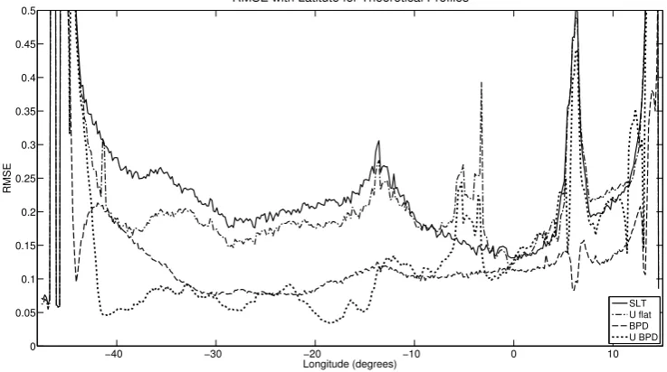
RMSE of the theoretical structure compared to the mean model structure at each longitude can be used to quantita-tively determine the quality of the fit between model and the-ory and is shown in Fig. 10. All the theories perform very badly at the boundaries, which may be due to the shallow water column and/or the rapidly changing gradients; however the behaviour of more interest is that in deep water regions. The SLT andU-Flat theories have very similar RMSE, with SLT more often having a higher RMSE i.e. a worse fit, al-though, particularly in the east, there are locations where the U-Flat has the higher RMSE. The BPD andU-BPD RMSEs are also similar, being generally lower than the SLT and U-Flat RMSEs, withU-BPD providing the best fit in the west while BPD generally provides a better fit in the east. BPD has the most consistent RMSE across the basin. Overall the theories including mean flow do better in the west than the no mean flow counterparts for the same topographic condition, however the situation is reversed in the east.
The RMSE can also be examined over depth, see Fig. 11, this provides an idea of the variability of the goodness of theoretical fit across the basin at each depth, effectively sum-marizing the errors seen in Fig. 9. Both theories including topography show very little error below 1500 m, however U-BPD shows a rapid increase in RMSE above that depth, con-sistent with Fig. 9d where alternating under and over estima-tion can be seen in this depth range. This gives a different
impression than when the theoretical profiles are subtracted from the model profiles (Fig. 7c), asU-BPD is the best the-ory over much of this depth range. BPD however performs well at the very surface, but has an increase in RMSE be-tween 200 and 1000 m associated with the too gentle surface intensification. SLT has a large RMSE at depth, which im-proves towards the surface, resulting in the lowest RMSE of all the theories in the 200 to 1000 m depth range, consistent with Fig. 9a. The RMSE of theU-Flat theory is intermedi-ate betweenU-BPD and SLT at depth and similar, although larger than,U-BPD at the surface. The addition of topogra-phy reduces the RMSE at depth, while the inclusion of mean flow increases the RMSE at the surface.
As made clear from the theoretical section, the vertical modal structures depend by construction on the zonal mean flow U, the buoyancy frequency N2, and the total ocean depthH, which all vary with longitude.
To investigate which factors might be influencing the er-rors, the correlation and the coefficient of determination (R2) is calculated between different variables and the section RM-SEs (Tables 3 and 4). The variables compared to the RMRM-SEs are: U, rawv, filteredv anomalies,N2, and topography. A significant correlation at the 99 % confidence level is found between the RMSE of all theories withU, raw v,N2 and topography. The significant correlations are all negative (i.e. the error increases as the value of the variable decreases) ex-cept forN2. The strongest correlations occur between the RMSE of all theories withUand topography, and addition-ally forU-Flat andU-BPD withN2.
TheR2 value indicates how much of the variance in the RMSEs can be accounted for by the variables. Particularly high values are again found for the correlations between all theories withUand topography, with the highest values for U-Flat withN2 and topography and betweenU-BPD with N2.
4 Discussion
Longitude (degrees)
Depth (m)
SLT minus Model Mean
−40 −30 −20 −10 0 10
0
2000
4000
−1 −0.5 0 0.5 1
Longitude (degrees)
Depth (m)
U Flat minus Model Mean
−40 −30 −20 −10 0 10
0
2000
4000
−1 −0.5 0 0.5 1
Longitude (degrees)
Depth (m)
BPD minus Model Mean
−40 −30 −20 −10 0 10
0
2000
4000
−1 −0.5 0 0.5 1
Longitude (degrees)
Depth (m)
U BPD minus Model Mean
−40 −30 −20 −10 0 10
0
2000
4000
−1 −0.5 0 0.5 1
Fig. 9. Theoretical sections (Fig. 8) minus the mean model section (Fig. 5c). (a) Standard linear theory minus the mean model section, (b)
mean flow with a flat bottom minus the mean model section, (c) no mean flow with topography minus the mean model section, and (d) mean flow and topography minus the mean model section. Contour interval is 0.05.
−40 −30 −20 −10 0 10
0 0.05 0.1 0.15 0.2 0.25 0.3 0.35 0.4 0.45 0.5
RMSE
Longitude (degrees)
RMSE with Latitute for Theoretical Profiles
SLT U flat BPD U BPD
Table 3. Correlation coefficient between the root mean square
er-rors of the theoretical sections compared to the model section for different variables. Correlations significant at 0.01 are in bold.
SLT U-Flat BPD U-BPD
RMSE RMSE RMSE RMSE
U −0.5 −0.6 −0.5 −0.6
Unfilteredv −0.4 −0.3 −0.4 −0.4
Filteredv 0.1 −0.1 0.1 0.0
N2 0.3 0.9 0.3 0.7
Topography −0.7 −0.8 −0.7 −0.8
this study the Radon transform was applied to a whole lat-itudinal section meaning the response is an amalgamation of the behaviours across the basin, while Lecointre et al. (2008) adopted a more localized approach, so it is possible that the assumption of a phase speed constant with depth is not ap-propriate in some individual locations or regions, but that as a generalized large scale approximation it is still valid. Al-ternatively, it is possible that the difference between our re-sults and those of Lecointre et al. (2008) simply stems from them using an automatic procedure for selecting peaks in the Radon transform that emphasizes criteria based on compar-isons with theoretical phase speeds and amplitude rather than vertical coherence. As discussed in this paper, it is clear that in the deep ocean, the dominant phase speed in the Radon transform is often different than at depths above. In some in-stances, the amplitude of the peak associated with the domi-nant surface phase speed may be small enough that it could easily be missed by an automatic detection procedure. In order to address the issue of vertical coherence more rigor-ously, what is needed is some form of statistical method that would test whether a given peak in the Radon transform can be regarded as statistically significant. In this paper, such tests were based solely on visual inspection, so that more work is needed to provide a more rigorous statistical basis to the approach. This is something that needs further investiga-tion and clarificainvestiga-tion to ensure assumpinvestiga-tions have a physical basis and are appropriate to the scale of investigation.
It is difficult to assess the realism of the vertical structures obtained from the model because of the lack of observations with a good vertical resolution (the very motivation for the study!), let alone observations coincident with the region of interest, and so confidence in the structures mainly comes from the similarities between the profiles constructed using different methods and the model’s proven ability to produce realistic Rossby waves (Lecointre et al., 2008) as well as pro-ducing recognizable first baroclinic forms.
The vertical structure found by Chu et al. (2007) used tem-perature data from ARGO floats in the North Atlantic and as a result is quite different to those found here with a pro-nounced sub-surface maximum at 1500 m and zero
ampli-Table 4. Coefficient of Determination (R2)for each of the root mean square errors of the theoretical sections compared to the mean model section for different variables.
SLT U-Flat BPD U-BPD
RMSE RMSE RMSE RMSE
U 0.24 0.36 0.23 0.39
Unfilteredv 0.24 0.10 0.22 0.19
Filteredv 0.01 0.01 0.01 0.00
N2 0.09 0.79 0.09 0.51
Topography 0.49 0.64 0.49 0.64
tude at the surface. Their findings showed a large contribu-tion from the second baroclinic mode in the structure, but did display a similarity to theU-BPD profile with an inver-sion seen in the top 200 m, which is not seen in the model profiles here. Hagen (2005) investigated the structure in the top 1000 m in the North Atlantic using dynamic depths and found the first baroclinic mode dominated while the second mode could be neglected where assumption of a flat bot-tom was reasonable but would have a significant contribution where topography is sharp. Here the second baroclinic mode was explicitly excluded to concentrate on the first baroclinic mode, although it does seem plausible that the second mode could be influential in this data, particularly because of the rough topography, as the second peak in the Radon trans-form is very comparable in amplitude to the peak selected and if, tentatively, interpreted as corresponding to the sec-ond mode would certainly contribute significantly to the sig-nal. This analysis could easily be repeated for the additional peaks seen in the Radon amplitude, which may provide fur-ther insight as to the skill of the theories.
in the northern rather than southern hemisphere, and if lati-tude alone were the influential factor the behaviour would be symmetric about the equator, resulting in comparable struc-tures. Local factors, such as topography, stratification and flow regimes, may act to mask such latitudinal dependence and are likely to be the main source of the discrepancies; but it is difficult to determine from the sparse data.
The resolution of the longitudinal structure of the verti-cal structure of Rossby waves is novel, illustrating the vari-ability across the basin, however since this is currently not achievable observationally the realism of these variations are unknown, although they still provide an interesting insight since just as the surface characteristics vary across the basin so would the underlying structures be expected to.
The longitudinal structure of the vertical profiles is not simple to explain. Similar patterns of deepening in the west are not seen in the density field of the model output, or the individual temperature and salinity fields. There is a slight shallowing of the pycnocline, thermocline and halocline in the east, however the scale of the variation is not compara-ble to that seen in the vertical profiles or at an equivalent depth. Nor does the structure reflect the bottom topography. The structures within the velocity fields also do not reflect the longitudinal structure. The case of this intense deepen-ing in the west is not only difficult to explain but is also not captured by any of the theoretical sections and examinations of hydrographic sections at similar latitudes also present no “real world” candidate for the cause of deepening. The use of un-validated model structures means it is unclear whether it is the theories or the model that is lacking in accurately describing the longitudinal structure.
The failings of the theoretical profiles compared to the model profiles are very similar in nature to those found by Aoki et al. (2009), who applied alternative methods to model data to determine the vertical structure of Rossby waves in the Pacific Ocean. Vertical structures were constructed us-ing model data from the Earth Simulator OGCM (OFES) and compared to the same four theoretical scenarios used here, although the effects of a finite wavelength were in-cluded, which is not considered here. In common with the findings here, using both mean flow and topography gener-ated the best fitting vertical profile, as shown by the profile RMSEs (Table 2) and qualitatively by their Fig. 8, however the surface fit of their mean flow and topography theory is better than that of the U-BPD profile as there is no inver-sion in the top 200 m, although they both show a common region of worse fit between 500 and 1000 m. The better fit seen with their mean flow and topography theory and model profile may be due to the inclusion of finite wavelengths, which needs much more investigation and consideration, or alternatively could be due to the model used representing Rossby waves in a different way to the CLIPPER model. Their standard theory produced a similar gross overestima-tion of the sign reversal at depth, as did including just mean flow, although to a lesser extent, which also produced the
too fast slow down at the surface seen in theU-Flat profiles. Their bottom pressure decoupling theory also displayed the too gradual reduction in amplitude with depth apparent in the BPD profile. Additionally the depths of the theories ap-proaching or passing zero are very comparable. The main contrasts between the Aoki et al. (2009) structures and those presented here is an obvious surface layer above 400 m af-ter which the amplitude remains constant for approximately 200 m down the water column, which is very different from the smooth reductions in amplitude presented here, although this is probably due to the differing density structures of the two oceans.
The RMSEs indicate that none of the theories are really adequately describing the model structures and in addition reveal that in different locations different theories are per-forming best, in general in the westU-BPD performs best, while in the east BPD is best, suggesting some aspects of the different theories are more appropriate for different loca-tions, possibly related to their differing conditions such as to-pography, velocities, density structure etc. It is clear however that with consistently the highest RMSEs (Table 2, Figs. 10 and 11), as has been discovered at the surface (e.g. Chelton and Schlax, 1996; Fu and Chelton, 2001), the standard linear theory is inadequate, except in the top 300 m of the vertical structure, where it performs the best (Figs. 6a, 9a and 11). Why this is the case is unclear as the assumptions seem no more valid in this layer than the rest of the water column.
The inclusion of topography is clearly the biggest factor in improving the agreement between model and theory as the BPD andU-BPD theories vie for lowest RMSE across the section (Fig. 10) while the improvement in RMSE of the in-dividual profiles from the SLT on the inclusion of topography (BPD) on average more than halves the RMSE, in compari-son to the inclusion of mean flow (U-Flat) resulting in a re-duction of less than 20 % from the SLT RMSE on average. The addition of mean flow to the topography (U-BPD) on av-erage improves the RMSE from the BPD RMSE by the same amount as between the SLT RMSE and the U-Flat RMSE suggesting that the improvements from mean flow and to-pography are additive and do not interact to effect the pro-file. This additive property only appears to hold on average for the vertical profiles. When Fig. 10, showing the RM-SEs for the sections, is examined it is clear the RMRM-SEs of U-Flat and BPD do not combine to produce the form of the U-BPD RMSE curve. In this case the effects of topography and mean flow do appear to interact differently at different locations affecting the skill of the theory at each point. How-ever the dominance of topography over mean flow in terms of improving the fit may be due to the location of the section as it has been suggested that equatorwards of 30◦mean flow may be less influential (e.g. Colin de Verdiere and Tailleux, 2005; Aoki et al., 2009).
0 0.2 0.4 0.6 0
500
1000
1500
2000
2500
3000
3500
4000
4500
5000
Depth (m)
RMSE with Depth for Theoretical Profiles
SLT U flat BPD U BPD
Fig. 11. Root mean square error of the theoretical sections
com-pared to the mean model section as a function of depth.
variability in error above 1500 m, further emphasising the dependence of the best theory with location. The source of the errors for each theory can be investigated by examining the correlation between different variables and the RMSEs. One of the highest correlations was found between all the-ories and the topography, with the relationship for thethe-ories including mean flow being slightly stronger, suggesting that while topography is the most important factor in reducing the RMSEs there are still shortcomings in how it is incorporated as shallower water increases the errors, leading to peaks in RMSE over the mid-Atlantic Ridge and Walvis Ridge. The R2analysis indicates that the topography could be account-ing for between 49 and 64 % of the error suggestaccount-ing this is an area that needs greater investigation and theoretical attention. The correlation between the mean flow and the RMSE is slightly weaker than for the topography but could still explain between a quarter and a third of the error, with higher values for theU-Flat andU-BPD cases. In this case since the major-ity of the zonal velocmajor-ity in this section is westward (i.e. nega-tive) the correlation coefficient indicates that the stronger the current the worse the error. This reinforces the importance of including mean flow but again its representation may need further investigation.
The vertical density structure as represented byN2 also has a strong correlation with the error, in particular for those theories including mean flow where extremely strong corre-lation is indicated by a correcorre-lation coefficient of 0.9 for the U-Flat theory. This indicates that the higher the value of
N2the higher the errors. In fact in the case ofU-FlatN2 could explain up to 79 % of the error variance, while it could explain around half the error in theU-BPD case, in severe contrast to a mere 9 % explained for the SLT and BPD theo-ries. Why stability of the water column would have a greater influence on the errors when mean flow is included is unclear. Interestingly the statistically significant correlation be-tween the RMSE and the unfiltered velocity suggests that the filtering may need to exclude less of the velocity data in or-der to capture the entirety of the variability within this mode. This could be aided in future by using the methodology of Aoki et al. (2009) that defines the region to filter by examin-ing the frequency-wavenumber spectrum of the data to select the signals that correspond to the theoretical dispersion rela-tions. The error this accounts for is between 19 and 24 %, ex-cept forU-Flat where it only accounts for 10 %. The addition of meridional velocity to the mean flow theoretical calcula-tions has been shown to produce little improvement to the agreement between theoretical and observed phase speeds (Killworth et al., 1997), although the effect on the 3-D struc-ture was not considered. This might explain why the percent-age of the error explained is relatively small for theU-Flat theory, while the higher value when topography is included with the mean flow may be due to topographic influence on the velocity. Including the meridional velocity may well pro-duce improvements in the way theory describes the vertical structure, however this is not simple as a finite meridional wave number would need to be defined, which could intro-duce further errors as it is generally poorly defined.
This study has focussed on how adaptations of linear the-ory affect the realism of the vertical structure they predict, however it must be noted that there are several other ap-proaches to Rossby waves, besides linear theory, for exam-ple, Paldor et al. (2007) examine non-quasigeostrophic ef-fects and Isachsen et al. (2007) investigate basin modes. The applicability of these theories could be investigated in future when more fully developed and generalized to 3-D.
its relevance, and suggests that the surface signature alone is not sufficient for that purpose.
5 Conclusions
– There is evidence to suggest that the assumption of a phase speed constant with depth is justified and may be valid for all modes, although further investigation is needed to confirm if this is the case for both local and large scales, as well as for other latitudes,
– using three different methods surface intensified vertical structures were identified, with some regions experienc-ing sign reversals at depth,
– the longitudinal structure revealed markedly different structures in the east and west Atlantic, with the west showing areas of no sign reversal or deep sign reversal, contrasted to the east where sign reversal consistently occurred between 1000 and 2000 m,
– the standard linear theory does not adequately describe the vertical structure because it grossly overestimates the amplitude of the sign reversal at depth, however a good fit is provided for the top 300 m,
– the addition of mean flow to the standard theory im-proves the agreement between model and theory by slightly reducing the overestimation of sign reversal at depth, but is too surface intensified leading to an under-estimation of the amplitude of the structure above the sign reversal,
– the addition of the effects of bottom topography to the standard theory gives an improved fit to both the stan-dard theory and the stanstan-dard theory plus mean flow by a more successful description of the structure at depth, however the surface structure reduces in amplitude too slowly consequently overestimating the amplitude of the structure above the sign reversal,
– combining the effects of mean flow and topography pro-vided the best fit for the individual model profiles, al-though an initial slight underestimation of the amplitude in the surface layer followed by a slight overestimation at mid depths are carried over from the individual ef-fects of mean flow and topography respectively, – over the length of the section the best fitting theory
varies between only topography and topography with mean flow, with, in general, topography only perform-ing better in the east,
– none of the theoretical profiles reproduce the deepening of the sign reversal in the west, although whether this is a shortcoming of the theories or the model, or both, is unknown due to lack of observational data,
– the generalization of this method to other latitudes, oceans, models and baroclinic modes would provide a greater insight into the variability in the ocean, while better observational data would allow verification of the model findings,
– additional theoretical considerations include the ef-fects of finite wavelengths, zonal propagation, non-quasigeostrophic effects and baroclinic instability along with the use of a wider range of measures of theoretical success than surface phase speed.
Acknowledgements. We are grateful to Paolo Cipollini for his
advice on the Radon method. Comments from two anonymous reviewers helped to improve the manuscript. R. T. acknowledges partial financial support from CNES.
Edited by: M. Hecht
References
Anderson, D. L. and Gill, A. E.: Spin-up of a stratified ocean, with application to upwelling, Deep-Sea Res. , 22, 583–596, 1975. Anderson, D. L. and Killworth, P. D.: Spin-up of a stratified ocean,
with topography, Deep-Sea Res., 24, 709–732, 1977.
Aoki, K., Kubokawa, A., Sasaki, H., and Sasai, Y.: Mid-latitude Baroclinic Rossby wave in a high-resolution OGCM Simulation, J. Phys. Oceanogr., 39, 2264–2279, 2009.
Barnier, B.: Forcing the Ocean, in: Ocean Modelling and Parame-terization, : Kluwer Academic Publishers, The Netherlands, 45– 80, 1998.
Chelton, D. B. and Schlax, M. G.: Global observations of Rossby waves, Science, 272, 234–238, 1996.
Chelton, D. B., Schlax, M. G., Samelson, R. M., and de Szoeke, R. A.: Global observations of large oceanic eddies, Geophys. Res. Lett., L15606, doi:10.1029/2007GL030812, 2007.
Chu, P. C., Ivanov, L. M., Melnichenko, O. V., and Wells, N. C.: On long baroclinic Rossby waves in the tropical North Atlantic observed from profiling floats, J. Geophys. Res. – Oceans , 112, C05032, doi:10.1029/2006JC003698, 2007.
Cipollini, P., Quartly, G. D., Challoner, P. G., Cromwell, D., and Robinson, I. S.: Remote sensing of extra-equatorial planetary waves, in: Manual of Remote Sensing Remote Sensing of Ma-rine Environment, editeb by: Gower, J. F., American Society for Photogrammetry and Remote Sensing, Bethesda MD, USA, 6, 61–84, 2006.
Colin de Verdiere, A. and Tailleux, R.: The Interaction of a Baro-clinic Mean FLow with Long Rossby Waves, J. Phys. Oceanogr., 35, 865–879, 2005.
Deans, S. R.: The Radon Transform and some of its applications, John Wiley, 1983.
Deser, C., Alexander, M. A., and Timlin, M. S.: Evidence for a Wind-Driven Intensification of the Kuroshio Current Extension from the 1970s to the 1980s, J. Climate, 12, 1697–1706, 1999. Fu, L.-L. and Chelton, D. B.: Large-scale ocean circulation.
Fyfe, J. C. and Saenko, O. A.: Anthropogenic speed-up of oceanic planetary waves, Geophys. Res. Lett., 34, L10706, doi:10.1029/2007GL029859, 2007.
Gill, A. E.: Atmosphere-Ocean Dynamics: Academic Press, San Diego 1982.
Hagen, E.: Zonal Wavelengths of Planetary Rossby Waves Derived from Hydrographic Transects in the Northeast Atlantic Ocean?, J. Oceanogr., 61, 1039–1046, 2005.
Hannachi, A., Jolliffe, I. T., and Stephenson, D. B.: Empirical or-thogonal functions and related techniques in atmospheric sci-ence: A review, Int. J. Climatol., 27, 1119–1152, 2007
Hirschi, J. J.-M., Killworth, P. D., and Blundell, J. R.: Subannual, seasonal and interannual variability of the North Atlantic merid-ional overturning circulation, J. Phys. Oceanogr., 37, 1246–1256, 2007.
Isachsen, P. E., LaCasce, J. H., and Pedlosky, J.: Rossby wave insta-bility and apparent phase speeds in large ocean basins, J. Phys. Oceanogr., 37, 1177–1191, 2007
Killworth, P. D. and Blundell, J. R.: The Dispersion Relation for Planetary Waves in the Presence of Mean Flow and Topography, Part II: Two-Dimensional Examples and Global Results, J. Phys. Oceanogr., 35, 2110–2133, 2005.
Killworth, P. D., Chelton, D. B., and de Szoeke, R. A.: The Speed of Observed and Theoretical Long Extratropical Planetary Waves, J. Phys. Oceanogr., 27, 1946–1966, 1997.
Lecointre, A., Penduff, T., Cipollini, P., Tailleux, R., and Barnier, B.: Depth dependence of westward-propagating North Atlantic features diagnosed from altimetry and a numerical 1/6◦model, Ocean Sci., 4, 99–113, doi:10.5194/os-4-99-2008, 2008. Paldor, N., Rubin, S., and Mariano, A. J.: A consistent theory for
linear waves of the shallow-water equations on a rotating plane in midlatitudes, J. Phys. Oceanogr., 37, 115–128, 2007. Pedlosky, J.: Geophysical Fluid Dynamics, Springer-Verlag, New
York 1979.
Penduff, T., Barnier, B., Dewar, W. K., and O’Brien, J. J.: Dynam-ical Response of the Oceanic Eddy Field to the North Atlantic Oscillation: A Model-Data Comparison, J. Phys. Oceanogr., 34, 2615–2629, 2004.
Picaut, J., Masia, F., and du Penhoat, Y.: An advective-reflective conceptual model for the oscillatory nature of the ENSO, Sci-ence, 277, 663–666, 1997.
Radon, J.: ¨Uber die Bestimmung von Funktionen durch ihre In-tegralwerte langs Gewisser Mannigfaltigkeiten, Berichte Sach-sische Akademie der Wissenschaften, Leipzig, Math.-Phys., 69, 262–267, 1917.
Rhines, P. B.: Edge-, bottom-, and Rossby waves in a rotating strat-ified fluid, Geophys. Fluid Dynam., 1, 273–302, 1970.
Rossby, C.-G. A.: Relation between variations in the intensity of the zonal circulation of the atmosphere and the displacements of the semi-permanemt centres of action, J. Mar. Res., 2, 38–55, 1939. Samelson, R. M.: Surface-intensified Rossby waves over rough
to-pography, J. Mar. Res., 50, 367–384 1992.
Smith, W. H. and Sandwell, D. T.: Global seafloor topography from satellite altimetry and ship depth soundings, Science, 277, 1957– 1962, 1997.
Taguchi, B., Xie, S.-P., Mitsudera, H., and Kubokawa, A.: Response of the Kuroshio Extension to Rossby Waves Associated with the 1970s Climate Regime Shift in a High-Resolution Ocean Model, J. Climate, 18, 2979–2995, 2005.
Tailleux, R.: Comment on: The Effect of Bottom Topography on the Speed of Long Extratropical Planetary Waves, J. Phys. Oceanogr., 33, 1536–1541, 2003.
Tailleux, R. and McWilliams, J. C.: The Effect of Bottom Pressure Decoupling on the Speed of Extratropical, Baroclinic Rossby Waves, J. Phys. Oceanogr., 31, 1461–1476, 2001.
Treguier, A. M., Reynaud, T., Pichevin, T., Barnier, B., Molines,J. M., de Miranda, A. P., Messager, C., Beismann, J. O., Madec, G., Grima, N., Imbard, M., and Le Provost, C.: The CLIPPER Project: High resolution modelling of the Atlantic, International WOCE Newsletter, 36, 3–5, 1999.