www.ocean-sci.net/11/719/2015/ doi:10.5194/os-11-719-2015
© Author(s) 2015. CC Attribution 3.0 License.
Global representation of tropical cyclone-induced short-term ocean
thermal changes using Argo data
L. Cheng1, J. Zhu1, and R. L. Sriver2
1International Center for Climate and Environment Sciences, Institute of Atmospheric Physics, Chinese Academy of Sciences, Beijing, China
2Department of Atmospheric Sciences, University of Illinois, Urbana-Champaign, IL, USA Correspondence to: J. Zhu ([email protected])
Received: 30 October 2014 – Published in Ocean Sci. Discuss.: 9 December 2014 Revised: 20 August 2015 – Accepted: 31 August 2015 – Published: 18 September 2015
Abstract. Argo floats are used to examine tropical cyclone (TC) induced ocean thermal changes on the global scale by comparing temperature profiles before and after TC pas-sage. We present a footprint method that analyzes cross-track thermal responses along all storm tracks during the period 2004–2012. We combine the results into composite repsentations of the vertical structure of the average thermal re-sponse for two different categories: tropical storms/tropical depressions (TS/TD) and hurricanes. The two footprint com-posites are functions of three variables: cross-track distance, water depth and time relative to TC passage. We find that this footprint strategy captures the major features of the upper-ocean thermal response to TCs on timescales up to 20 days when compared against previous case study results using in situ measurements. On the global scale, TCs are responsible for 1.87 PW (11.05 W m−2)of heat transfer annually from the global ocean to the atmosphere during storm passage (0– 3 days). Of this total, 1.05±0.20 PW (4.80±0.85 W m−2)
is caused by TS/TD and 0.82±0.21 PW (6.25±1.5 W m−2)
is caused by hurricanes. Our findings indicate that ocean heat loss by TCs may be a substantial missing piece of the global ocean heat budget. Changes in ocean heat content (OHC) after storm passage are estimated by analyzing the tem-perature anomalies during wake recovery following storm events (4–20 days after storm passage) relative to pre-storm conditions. Results indicate the global ocean experiences a 0.75±0.25 PW (5.98±2.1 W m−2)heat gain annually for hurricanes. In contrast, under TS/TD conditions, the ocean experiences 0.41±0.21 PW (1.90±0.96 W m−2)ocean heat loss, suggesting the overall oceanic thermal response is par-ticularly sensitive to the intensity of the event. The ocean heat
uptake caused by all storms during the restorative stage is 0.34 PW.
1 Introduction
Tropical cyclones (TCs) provide an effective mechanism to transport heat, mass and nutrients in the ocean, while also exchanging enthalpy with the atmosphere. Multiple lines of evidence from previous observational and modeling studies indicate that these relatively small-scale and transient events can influence large-scale dynamical processes in both the ocean (Emanuel, 2001; Sriver and Huber, 2007) and the at-mosphere (Camargo and Sobel, 2005; Hart, 2011; Jansen et al., 2010; Sriver and Huber, 2010)
the ocean than in the atmosphere. On synoptic scales, TC-induced cooling at the surface via enhanced mixing can limit TC intensification (e.g., Ginis, 2002).
Understanding the ocean’s response to TCs on various spatial and temporal scales is an ongoing area of active re-search. Since the 1950s, ocean vessels, moorings, and air-craft have been observing ocean conditions in TC-affected regions, which has assisted in building the basic framework for understanding how the ocean responds to TC forcing (Black and Dickey, 2008; Price, 1981, 1983; Price et al., 1994; Shay and Elsberry, 1987; Shay et al., 1989). The re-sponse of the upper ocean to TC forcing is typically charac-terized by surface cooling in the storm wake and subsurface warming caused by a variety of oceanic and atmospheric pro-cesses, including generation of near-inertial internal oscilla-tions, geostrophic advection, Ekman pumping, and surface fluxes. Previous studies analyzing the ocean response to TCs have generally been limited by the availability of observa-tions and/or focus on a limited number of storms, resulting in storm-to-storm variations (Bell et al., 2012; Cione and Uhlhorn, 2003; Lin et al., 2009a, b). Until recently, these lim-itations in data coverage have prevented a global-scale per-spective of how TCs affect the ocean.
Previous efforts to quantify the impact of TCs on upper ocean heat content (OHC) have relied primarily on near-surface observations (Sriver and Huber, 2007; Sriver et al., 2008; Jansen et al., 2010) and altimetry sea level data (Mei et al., 2013), inferring a redistribution of heat via vertical mix-ing. Because there is a relatively firm theoretical understand-ing of the ocean’s response to TC wind forcunderstand-ing (Price, 1981), global sea-surface temperature (SST) fields from satellites and reanalysis serve as the basis for first-order estimates of TC impacts, because they offer global coverage and rela-tively high spatial and temporal resolution. But, these meth-ods come along with fundamental assumptions about the in-terior ocean response. For example, Sriver and Huber (2007) assume that the upper 50 m depth ocean is cooled homoge-neously within TC cold wakes, reflecting the temperature change observed at the surface, and all cooling is achieved through vertical mixing. Given these assumptions, they es-timate that 0.2–0.4 PW of heat is transported into the ocean interior globally. Using improved methodologies, several ad-ditional observational studies have generally supported this result (Jansen et al., 2010; Sriver et al., 2008; Mei et al., 2013).
A key uncertainty missing in the above studies is the effect of enthalpy exchange at the air–sea interface (Emanuel, 1991, 1999). Typically these fluxes are estimated by measuring the humidity near the sea surface using mooring instruments and calculating the latent heat flux according to a parameterized bulk equation. A so-called drag coefficient is needed to ap-proximate the efficiency of heat transfer, which is one of the sources of uncertainties in the high-wind weather con-ditions (Powell et al., 2003). Another source of uncertainty arises due to the spatial and temporal variations in humidity,
temperature and wind speed under highly chaotic wind con-ditions, since the winds undergo rapid changes in direction and magnitude in TC conditions (Wright et al., 2001). Ad-ditionally, the effect of sea spray must also be taken into ac-count, since it represents an efficient mechanism transporting enthalpy in the air–sea boundary layer under strong winds. These uncertainties make the direct measurements of the air– sea fluxes difficult, and thus it is perhaps necessary to ac-cumulate large numbers of measurements to achieve statis-tically significant results. Despite these limitations, studies have shown that the air–sea heat fluxes within TCs are on the order of 2 to 3 times greater than the background heat fluxes in quiescent conditions (D’Asaro, 2003; Lin et al., 2009). These studies improve the understanding of the air–sea heat exchange by TCs, but global-scale estimates are difficult.
Following the surface drag methods, Trenberth and Fa-sullo (2007) use a high-resolution model to examine the TC-induced water and energy budgets on the global scale. Their estimate of heat flux is based on an empirical relationship between heat flux and wind speed (Trenberth et al., 2007). They find that 0.17 PW heat is released from the ocean to the atmosphere within 400 km of the storm center, and 0.58 PW within 1600 km.
These previous studies suggest that TCs induce a sub-stantial amount of heat exchange between the atmosphere, oceanic mixed layer, and upper thermocline; thus, these events may play an important role in influencing global heat budgets and climate. However, comprehensive global esti-mates of air–sea exchanges, ocean interior thermal changes, and net effects on OHC have not yet been estimated using global, vertically resolved ocean observations.
A key difficulty in quantifying the global distribution of TC-induced oceanic thermal response is the lack of all-weather observations with sufficient horizontal, vertical and temporal coverage and resolution. Since the year 2000, Argo profiling floats have provided a global network of in situ ocean surface and subsurface observations (von Schuckmann and Le Traon, 2011; Willis et al., 2009). The profiles mea-sure water temperature and salinity from the surface (∼5 m) to∼2000 m depth, even under extreme weather conditions such as TCs. Since 2004, the Argo system has maintained a global array network with a resolution of about 3 by 3◦ in space similar to the XBT-based system (Freeland et al., 2009). However, the main advantage of the Argo system over previous observational systems is that the floats are more evenly distributed in space and time over the ocean and can observe conditions from greater depths.
from a series of Argo data near the storm. These results sup-port the reliability of Argo observations in severe weather conditions. More recent work examining TC-induced ocean heat content changes in the western Pacific (Park et al., 2011) represents the first attempt to investigate systematically the TC-induced ocean thermal changes on a basin scale using Argo data. While the authors do identify a TC signature in the Argo data, the TC-induced subsurface temperature response is sensitive to the season in which TCs occur. Furthermore, the TC-induced effect is difficult to separate from the back-ground variability, particularly for weak storms.
Here we present a new method to examine global TC– ocean interactions using Argo data that examines all storms globally and characterizes the global mean of the cross-track ocean response to TCs using a footprint method that fol-lows along the storm tracks. We categorize the TC events into two separate groups: tropical storms/tropical depressions (TS/TD) and hurricanes. In addition, we separate the ocean’s response into two stages: the forced stage (0–3 days relative to storm passage) and the recovery stage (4–20 days rela-tive to storm passage). We use this technique to analyze TC-induced ocean thermal responses and latent heat fluxes on a global scale, accounting for regional variability in back-ground ocean conditions. The paper is organized as follows. We describe the data and footprint methodology in Sect. 2. We present the results and discussion in Sect. 3. We discuss the caveats of the method in Sect. 4, and Sect. 5 outlines the main conclusions.
2 Data and methods 2.1 Data
Argo floats drift freely at a fixed pressure (usually 1000 m depth and occasionally at 1200 and 1500 m) for about 9– 10 days. After this period, the floats descend rapidly to a profiling pressure (usually 2000 m deep) and then rise, col-lecting near-instantaneous profiles of pressure, temperature, and salinity data on their way to the surface (within a span of about 2 h). The floats remain at the surface for less than 1 day, transmitting the data collected via a satellite link back to a ground station and allowing the satellite to determine their surface positions. The floats then sink again to a park-ing depth of∼1000 m and repeat the cycle.
Argo data are available on the website of the National Oceanographic Data Center/Global Argo Data Repository. In this study, we use Argo data from January 2004 to De-cember 2012 (downloaded on October 2013). We discard all the profiles in the so-called grey list (Willis et al., 2009), within which the Argo floats with pressure drift error are listed. Both delayed mode (data available several months af-ter passing careful quality control processes) and real-time mode (data available to users within a 2-day time frame) data are used where available, and Argo quality control flags are used to eliminate spurious measurements. We apply an
addi-tional boundary check as follows. If a temperature anomaly within 200 to 1000 m from a pair (discussed in more detail in Sect. 2.2) is larger than 2◦C (or smaller than−2◦C), the anomaly is labeled “spurious”. If there are more than five “spurious” labels from a single pair, the pair is rejected and all of the “spurious” anomalies are removed. This is a widely used quality control process and helps to get rid of the spikes and anomalous profiles.
Tropical cyclone information comes from the NOAA’s Tropical Prediction Center “best track” data set (http:// weather.unisys.com/). The data set contains 6-hourly records of maximum wind speeds, pressure and location. We collect all TC tracks globally between January 2004 and December 2012, totaling 885 events.
2.2 Composite footprint method
We introduce a footprint method that averages all of the TC-induced cross-track (i.e., perpendicular to the storm’s direc-tion of modirec-tion) ocean temperature changes. Argo pairs are selected to compare temperature profiles before and after storm passage according to the following criteria.
1. The pre-storm Argo profile is within−12 to−2 days before storm passage and the post-storm Argo profile is within 0 to 20 days after storm passage. The 20-day limit is selected because SST changes are largely restored to pre-storm conditions within 20 days after storm passage. Furthermore, it is increasingly difficult to separate TC effects from the seasonal cycle of SST on timescales longer than 20 days. Data within−2 to 0 days prior to storm passage are not used as pre-storm reference profiles, since they may be affected by TC processes (e.g., increased heat fluxes ahead of storms) and horizontal advection (Huang et al., 2009).
more than 0.2◦ away from its original position on the timescales of our TC analysis. Thus, the maximum 0.2◦ spatial constraint largely filters these floats from our re-sults, so that we do not contaminate the TC analysis with transient effects of larger-scale dynamics.
3. All of the Argo pairs are within 8◦relative to the center of the storm track, perpendicular to the storm’s direc-tion of transladirec-tion. Thus, 16◦is assumed to be the maxi-mum cross-track scale of the area affected by TCs. This constraint is a first-order assumption, and we will an-alyze the horizontal scale of the globally averaged TC response extensively in the results section. Additional information about the composite footprint method can be found in Appendix A.
The footprint method outlined above features several key methodological limitations, which include (i) neglecting along-track TC-induced ocean variability; (ii) lack of Argo float comparisons within individual storms due to poor sam-pling at these spatial and temporal scales; and (iii) the ef-fect of background ocean variability at specific sampled loca-tions, which is difficult due to the sparseness of the floats and the frequency of the measurements. A sensitivity test on the effect of background variability is presented in Appendix B, indicating that there is no significant systematic bias induced by background variability when using the footprint method. 2.3 Estimation of ocean heat content changes during
0–3 days after storm passage
Since the air–sea exchanges in the TC affected regions within 0–3 days of the storm passage are dominated by TC effects, which are several times larger than the background air–sea heat exchanges, it is reasonable to assume that the net ocean heat change within the TC-affected regions during this pe-riod is totally induced by TCs. Our choice of 3 days is to, at least partially, average out any float drift caused by iner-tial oscillations. This strategy is based on the notion that the ocean must be the energy source of a storm, so the total heat loss in the ocean during the storm is transported to the air as air–sea heat flux during the storm passage (0–3 days). The averaged OHC change is calculated as follows (in Watts):
QATSTD=Ltrack−TSTD[ dist=8
Z
dist= −8 1
T3 days
δt=3
Z
δt=0
depth=1200
Z
depth=0
ρcpFTSTD(dist,depth, δt )ddepthdδtddist]/Tyear,
QAHur=Ltrack−Hur[ dist=8
Z
dist= −8 1
T3 days
δt=3
Z
δt=0
depth=1200
Z
depth=0
ρcpFHur(dist,depth, δt )ddepthdδtddist]/Tyear, where cp is heat capacity of seawater ∼4186 J kg−1◦C; ρ is density of seawater, which is calculated using Argo salin-ity, pressure and temperature measurements before the storm;
Tyearis the duration of one calendar year in seconds, to cal-culate an annual mean; andLtrack−TSTD andLtrack−Hur are averaged track length within 1 year, about 1.4×10⁸m and 8.3×10⁷m for TS/TD and hurricanes, respectively, which are obtained by averaging the track length from 2004 to 2012. We choose the time period between 0 and 3 days, be-cause it likely captures the majority of the air–sea heat ex-change during storm passage. However, other mechanisms may also influence air–sea heat flux in this time period, such as storm-induced cooling via mixing and wave generation. TC-induced surface cooling can cause a reversal of surface fluxes in the days following storm passage, which marks the transition between the forcing stage and the recovery stage. Some studies suggest fluxes may reverse sign around 2 days after TC passage (Dare and McBride, 2011; Lloyd and Vec-chi, 2011). The exact timing of this reversal depends on many factors, such as storm intensity, translation speed and re-gional conditions, and the best choice is unclear in a global context. We performed sensitivity tests of the TC response to different choices of the time length (0–2, 0–2.5, 0–3.5 and 0–4 days), and the results (not shown) and interpretations are generally consistent for all timescales.
2.4 Estimation of air–sea fluxes during TC passage We examine the air–sea heat transfer rate in the TC-affected regions by averaging air–sea heat flux as follows (in W m−2):
HTSTD=QATSTD/(Ltrack−TSTD×R), HHur=QAHur/(Ltrack−Hur×R),
whereRis the cross-track size of the TC-affected region that is set to be 16◦ (±8◦across the track). The other variables are consistent with QATSTDand QAHur.
2.5 Estimation of ocean heat content changes during 4–20 days after storm passage
Figure 1. Count of TC-affected pairs in each 0.5◦ distance bin from−8◦to 8◦ across the storm track for two footprint compos-ites: TS/TD in the upper panel, hurricanes in the bottom panel. The statistics are conducted in two time periods: 0–3 days on the left, 4–20 days on the right.
We calculate OHC changes using (in Watts)
QNTSTD=Ltrack−TSTD[ dist=8
Z
dist= −8 1
T17 days
δt=20
Z
δt=4
depth=1200
Z
depth=0 ρcpFTSTD(dist,depth, δt )ddepthdδtddist]/Tyear,
QNHur=Ltrack−Hur[ dist=8
Z
dist= −8 1
T17 days
δt=20
Z
δt=4
depth=1200
Z
depth=0 ρcpFHur(dist,depth, δt )ddepthdδtddist]/Tyear,
where T17 days is the duration of 17 days in seconds. The other variables are the same as those in calculating QATSTD and QAHur.
Limitations of this methodology include the following. 1. The OHC changes induced by TCs are averaged within
4 to 20 days after storm passage, which approximately represents the restoration stage. However, the ocean changes may not be fully restored during this time inter-val. As noted previously, we choose this time period be-cause TC signals are difficult to separate from the back-ground seasonal cycle on longer timescales.
2. The internal waves generated by TCs induce fluctua-tions in temperature, which could potentially bias our results. However, we hypothesize that these wave ef-fects average to zero because we are using a large num-ber of Argo pairs (∼4410).
3 Results and discussion
Here we present the three-dimensional footprint maps for two time intervals, 0–3 and 4–20 days referenced to storm passage. The 0–3-day interval represents about two inertial periods and reflects the direct ocean response to storm forc-ing (Sanford et al., 2011). We choose 3 days as an upper limit to the forced stage based on the following methodological constraints, limitations and uncertainties: (1) TC track infor-mation is every 6–12 h, and Argo data may be offset by sev-eral hours due to their ascent speed; together these effects can lead to observational offsets of up to 1 day; and (2) the iner-tial period changes rapidly with latitude in TC-affected re-gions (from 1 to 3 days). Considering these uncertainties, we choose 3 days as an approximation of the forced stage on the global scale, which represents the initial period of the TCs’ influence on upper-ocean properties. We have conducted ad-ditional sensitivity tests to the choice of forced stage time interval using −1 to 2 days relative to storm passage, and the results are generally consistent with the results presented here.
After 4 days, the ocean typically begins recovering to pre-storm and/or climatological conditions. While this restora-tion period can persist from weeks to months (Mei et al., 2013; Mei and Pasquero, 2013), this analysis averages the thermal response between 4 and 20 days after storm pas-sage to estimate the mean ocean response during the recovery stage. Anomalies for both forced and recovery stages are ref-erenced to pre-storm conditions as discussed in the methods section.
The amount of data for each footprint composite for the two time periods is shown in Fig. 1. In the upper 100 m, the number of measurements is generally more than 30 in each 0.5◦ box, except near the storm center. The measurements generally decrease with depth, especially deeper than 1000, 1200 and 1500 m (parking depths).
3.1 The 0–3-day footprint of ocean thermal changes During storm passage, in the so-called forcing stage (Price et al., 1994), the cyclonic winds generally pump cold wa-ter up to the surface near the storm eye (Ekman pumping) and generate divergent currents in the upper ocean. To com-pensate for the upwelling, downwelling away from the track occurs over a large area, appearing as ocean warming in the subsurface regions. Meanwhile, the strong and sudden distur-bance of storm winds generates near-inertial horizontal cur-rents (Shay and Elsberry, 1987) whose vertical shear leads to cold-water entrainment at the base of the mixed layer.
a
b
a
b
c
b
a
d
Figure 2. The 0–3-day averaged thermal changes (relative to pre-storm conditions) as a function of depth and distance, in TC track coordinates. (a) TS/TD, between+5 and−5◦from the track center; the dashed contour interval is 0.1◦C, and the solid black contours isolate the 90 % confidence interval of the signals. The standard er-ror of the footprint is presented in (b). (c) is the 0–3-day footprint for hurricanes, between±7◦from the track center, the dashed con-tour interval is 0.2◦C, and the solid black contours isolate the 90 % confidence interval of the signals. The standard error of the footprint is presented in (d). The unit is◦C.
on the right side of the track (in track coordinates). A much weaker pattern is found on the opposite side, supporting the asymmetry of the ocean response documented previously in the literature. These near-surface cooling signals have uncer-tainties (standard errors in Fig. 2b, d) with magnitudes of less than 40 % of the signals. The rightward-biased cooling in the track coordinate system near the surface is also found in pre-vious studies (left side in the Southern Hemisphere) (Dare and McBride, 2011; Price, 1981, 1983; Sanford et al., 2011; Dickey et al., 1998) due to the stronger vertical shear in the right side of the track. This mechanism contributes∼80 % of the SST response (Price et al., 1994). Another cooling mech-anism besides the shear instability is the turbulence also gen-erated by wind stress (Chan and Kepert, 2010). Both are irre-versible processes that produce mixed-layer deepening. The mixing transports heat vertically from the sea surface to the subsurface, appearing as a subsurface warming correspond-ing to the near-surface coolcorrespond-ing, which is apparent in Fig. 2 with a peak at∼50–100 m.
Figure 2 shows a subsurface (30–200 m) cooling within 1◦of the track, and a subsurface warming on both sides of the track between±2 and 4◦from the storm center, consis-tent with previous results (e.g., Price, 1981; Sanford et al., 2011). These warming signals contain relatively large uncer-tainties (the standard error ranges from 40 to 100 % of the absolute value of the signals) compared with surface signals, partly because they occur within the thermocline that exhibits
−8 −7 −6 −5 −4 −3 −2 −1 0 +1 +2 +3 +4 +5 +6 +7 +8 −1.2
−1 −0.8 −0.6 −0.4 −0.2 0 0.2 0.4
Distance (degree)
Temperature anomaly (
oC)
TS/TD 0−20m Hurricane
TS/TD 0−1200m Hurricane 0−1200m TS/TD
Hurricane 0−20m
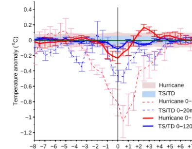
Figure 3. The 0–3-day averaged temperature change as function of distance across the cyclone center for hurricanes (red) and TS/TD (blue), in TC track coordinates. The values are smoothed using a three-point (1.5◦) moving filter. Light blue shading shows the 90 % confidence interval of background noise based on null-hypothesis analyses for TS/TD, and the light pink shading is for hurricanes. Surface temperature anomalies are presented as the thin curves, and the thick curves show 0–1200 m averaged temperature changes. The error bars are 1 SD, which is calculated as follows: 90 % percent of pairs are randomly selected, and then we calculate the thermal anomalies of these pairs. This process is repeated 200 times, so 200 samples of thermal anomalies are obtained, and the SD is calculated from thermal anomalies of these 200 samples.
higher variability. Our composite analysis of the response from Argo floats confirms that there is an Ekman pumping effect in the upper ocean (upper 200 m), in that we observe a residual vertical motion within 1◦of the storm track, appear-ing as a net column-averaged coolappear-ing near the storm center, along with downwelling outside the storm center (Fig. 2a and b). It is also possible that instantaneous wind erosion plays a role in addition to upwelling (Jacob and Shay, 2003; James et al., 2011) for the upper ocean changes (upper 200 m), in particular during slower storms that produce weaker near-inertial velocity responses. Despite smoothing out of near-inertial oscillations, the resultant subsurface warming is observable. At depths greater than 200 m, we find a weak cooling sig-nal near the storm center and weak warming away from the storm. The weak cooling near the storm center (between−1 and+1◦) is significant down to 400 m for hurricanes and 200 m for TS/TD. These signals have large uncertainties, with standard errors up to 100 % of the signals (Fig. 2d). The causes of these deep ocean responses are beyond the scope of this study, but they may be linked to vertically propagat-ing waves (Ascani et al., 2010; Sriver et al., 2013). Compar-ison of the TC thermal response with background oceanic variability indicates that the major structure of TC-induced thermal changes is significant compared with the background variability, as highlighted by black lines in Fig. 2a, c.
to storm passage (Fig. 3), and we highlight the different char-acteristics of the response of the upper ocean (0–20 m) versus the entire column depth. Near the surface (0–20 m), for hur-ricanes, the cooling spreads to a large area of±5◦from the storm center, with a peak around∼ −1.1◦C. In contrast, for TS/TD, we observe less cooling over a smaller area (a peak of∼ −0.5◦C). The sea surface anomalies estimated by Argo observations are consistent with other SST observations pre-sented by multiple previous studies (Lloyd and Vecchi, 2010, 2011; Mei and Pasquero, 2013).
For the response of the entire ocean column, TS/TD gener-ally cause cooling between−1 and+3◦in storm coordinates, implying that the dominant mechanism affecting column-integrated temperature changes in TS/TD-affected regions is surface fluxes. The wind-driven entrainment itself does not change the ocean heat content of the whole water column, instead re-distributing the heat vertically via mixing. Ocean currents also advect mass and heat from their origin to differ-ent locations, but do not change the net ocean heat contdiffer-ent. Therefore, if there is a net ocean heat content change over a TC-affected region, it must be via the ocean–atmosphere sur-face heat fluxes. A significant heat flux is also found in pre-vious studies (Bell et al., 2012; Lin et al., 2009b; Mcphaden, 2009), and we expand on this discussion in the next section.
For hurricanes, the water column experiences a cooling within ±2◦of the storm center, and stronger warming near between +2 and +4◦ along the right side of the track (in track coordinates). Both cold and warm peaks are significant at the 90 % confidence level according to the null-hypothesis tests (see Appendix C). This implies that there is a net heat transport from the storm center to the right side of the storm relative to the storm’s direction of motion. The magnitude of column-averaged cooling (within +2◦ of the storm center) is greater than the warming along the right side (+2∼4◦); thus, the net effect is a cooling of the upper ocean through enhanced surface fluxes.
3.2 Estimate of air–sea heat flux
Here we calculate a global estimate of air–sea heat exchange during TCs by integrating the ocean heat differences within storm-affected regions during a 3-day interval surrounding storm passage. We assume that during this period, the net column-integrated ocean heat loss is caused by heat trans-fer from the ocean to the atmosphere. We use the foot-print methodology, which has two spatial dimensions: ver-tical depth and cross-track distance relative to the storm’s direction of motion. Thus, the footprint represents a two-dimensional insulated box that is±8◦across the storm track relative to the storm center and 1200 m deep, with an open-ing at the air–sea interface. The heat exchange between the box and its surroundings occurs only at the surface.
To test whether assumptions about the footprint hold, par-ticularly related to insulation from horizontal advection at the sides of the box and vertical heat exchange at the base, we
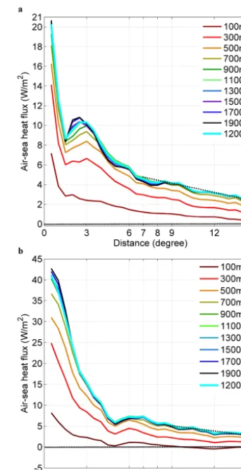
Figure 4. Estimates of air–sea heat flux within TC with different footprint domain sizes (horizontal and depth) for (a) TS/TDs and (b) hurricanes. The results of 1200 m are highlighted in cyan.
calculate the box-averaged air–sea heat flux at different hor-izontal and vertical spatial scales, ranging from dx= ±1◦to ±15◦(with 0.5◦increment) and dz=100 m to 1900 m (with 200 m increment). As shown in Fig. 4, the averaged air– sea heat flux stabilizes for dx>∼6◦. The decreasing trend for dx>∼7◦ is a “dilution” effect, which is caused by en-larging the box size while the OHC change within a TC-affected region remains unchanged. Note this effect is gen-erally linear for large dx, which is expected since the depth is held constant. In the vertical direction, the air–sea flux esti-mates are unchanged for dzgreater than 700 m (correspond-ing to dx>∼5◦). This result suggests the method requires at least ±7◦ and 700 m in order for the insulated box as-sumption to be considered valid. Thus, we use a terminal depth dz=1200 m based on the availability of data in the upper ocean (a large portion of Argos stop near 1200 m), and dx=8◦.
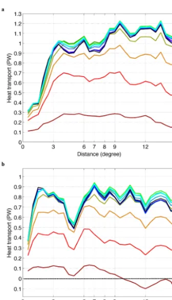
cal-Figure 5. The impacts of domain size on global annual heat trans-fer from the ocean to the atmosphere by TCs for (a) TS/TDs and (b) hurricanes. The colors are the same as those in Fig. 4.
culate the total global air–sea heat exchange in Fig. 5. Given the methodology described previously, the integrated heat transport should converge to the total TC contribution, as we increase the domain size. Consistent with Fig. 4, this con-vergence occurs for dx>∼6◦. For TS/TD, heat exchange continues to increase to dx> 9◦. However, this increase is probably not caused by TCs given the large spatial scale. Therefore, we estimate the global annual air–sea heat ex-change during TCs to be 1.05 and 0.82 PW for TS/TD and hurricanes, respectively. The total heat transfer is 1.87 PW annually, which represents the total heat loss from ocean to atmosphere during the forced stage (0–3 days).
The global air–sea fluxes derived in Fig. 4 correspond to 584 W m−2 for TS/TD and 761 W m−2 for hurricanes, when averaging fluxes within storm-affected regions (±8◦ across the track). These values are consistent with previ-ously published case study estimates, such as the mooring observations during the category-4 hurricane Nargis (Lin et al., 2009; Mcphaden et al., 2009), which estimated storm-induced air–sea fluxes of ∼400–900 W m−2. Furthermore, our global estimates are consistent to first order with the estimated heat required to bring the troposphere into ther-modynamic equilibrium (Emanuel, 1991) with the ocean of ∼108J m−2, which is equivalent to∼3 W m−2annually over the global ocean basin. This estimate generally agrees
0 50 100 150-60 -30 0 30 60
Watts/m^2
a. b.
-1 0 1-60 -30 0 30 60
Watts/m^2
c. d.
Figure 6. Geographical pattern of air–sea heat flux caused by TCs. (a) Globally integrated heat flux caused by TCs calcu-lated using Argo float data (W m−2). (b) Zonally averaged TC-induced heat flux (red curve), compared with the annual climatol-ogy (1990–2010) of air–sea latent heat flux (black curve) derived from NCEP/NCAR reanalysis (Kalnay et al., 1996). (c) Surface flux (positive upward) along storm tracks for climatological conditions during the period 1990–2010 (W m−2), derived from NCEP/NCAR reanalysis using storm tracks from 1990 to 2010. The plot represents the background air–sea flux contribution to the Argo analysis using the 20-year daily climatology. (d) Zonal average of the climatolog-ical net surface heat fluxes shown in (c).
a
b
Figure 7. Frequencies of tropical cyclones per year affecting 1◦ by 1◦grid boxes, when the TC-affected region is assumed to be (a)±1◦from the track center and (b)±8◦from the track center.
The geographical patterns of the TC-induced air–sea heat fluxes are presented in Fig. 6, using spatial and temporal av-eraging consistent with our global estimates. We find signif-icant spatial variability in the flux estimates, with the largest fluxes occurring in regions with the most TC activity (i.e., the northwestern Pacific). These results indicate that the zon-ally averaged TC contribution to the total annual air–sea en-thalpy flux budget may be as large as ∼9.1 W m−2, with peak values of around 20 W m−2at latitudes experiencing the most TCs. These fluxes could account for as much as∼10 % of the total annual ocean latent heat flux (90–110 W m−2) (Trenberth et al., 2009) derived using NCAR/NCEP reanaly-sis (Kalnay et al., 1996), shown as the black curve in Fig. 6b. As a simple check of the TC contributions of net sur-face fluxes, we compare the results from Argo data to the background surface fluxes using the NCEP/NCAR reanal-ysis. Specifically, we calculate the net climatological air– sea heat fluxes along TC tracks using NCEP/NCAR reanal-ysis for the same Argo sampling criteria (dx=8◦, dt=0– 3 days). However, these climatological fluxes represent the daily averages over a 23-year period (1990–2012), rather than from specific TC days. In other words, the plot shows the surface fluxes along storm tracks for non-TC conditions. The NCEP/NCAR reanalysis product generally predicts a net oceanic heat uptake in background climatological conditions during TC seasons (Fig. 6c). In the absence of TCs, typical conditions would favor a net ocean heat uptake on the order of 1 W m−2zonally averaged across the global ocean. This background warming signal is of opposite sign to the TC ef-fect, which tends to cool the ocean through enhanced surface fluxes during the forcing stage.
Figure 6a shows a prominent peak in air–sea heat flux in the western Pacific Ocean, reaching values as large as 65 W m−2. Because this region experiences the most TC
ac-
W/m2
Figure 8. Geographical distribution of air–sea heat flux caused by TCs. We assume each grid box can only be affected by one storm within a 20-day window.
tivity, this peak is probably due to more TC occurrences rel-ative to other regions.
In Fig. 7a and b, we present the frequency at each 1◦by 1◦ grid box that is affected by TCs per year, given the affected regions (cross-track distance) defined to be±1 and±8◦ rel-ative to the storm center. As expected, the figure shows a higher frequency of TC occurrences in grid boxes as we in-crease the size of the affected region. For example, in the western and eastern Pacific Ocean, between 1 and 1.5 storms pass directly through a single 1◦by 1◦grid box annually, but this activity can contribute as many as 12∼14 storms affect-ing the same grid boxes when we increase the TC-affected region to±8◦.
To check whether the peak in heat flux is caused by in-creased frequency of TCs, we assume that one grid box can be affected by only one storm within 20 days. The annual air–sea heat fluxes for this method are presented in Fig. 8, showing that the peak fluxes in the northwestern Pacific de-crease to 30 W m−2, while the overall fluxes in the other basins are relatively unaffected (to within∼5–10 W m−2). Since the nature of air–sea heat exchanges is complicated by the close proximity of storms in active TC regions, such as in the northwestern and northeastern Pacific, our geographical map of air–sea heat flux should be regarded as a first-order approximation.
hurri-c
a b
d
Figure 9. Two-hundred estimates of heat transport (in a and c) and air–sea heat flux (in b and d) based on 200 randomly selected sam-ples of pairs. (a) and (b) are estimates under TS/TD conditions and (b) and (c) for hurricanes. The mean of 200 estimates is highlighted in blue for TS/TD and in red for hurricanes. Error bars represent the standard error.
canes (Fig. 9a, c), which is equivalent to ∼20 and∼25 % of the total estimates for TS/TD and hurricanes, respectively. Including these uncertainties, our estimates of air–sea heat flux during the TC forcing stage (0–3 days relative to storm passage) are 1.05±0.20 PW (4.8±0.85 W m−2)for TS/TD and 0.82±0.21 PW (6.25±1.5 W m−2)for hurricanes.
3.3 The 4–20-day footprint of ocean thermal changes After storm passage, radiative forcing and ocean currents tend to restore the storm-induced surface anomalies. Past studies show that upocean thermal anomalies can per-sist on the order of 10–20 days (Price et al., 2008), 20– 30 days (Dare and McBride, 2011), or even longer than 30 days (Mei et al., 2013; Mei and Pasquero, 2013; Park et al., 2011). Differences in timescales likely depend on differ-ences in regional and seasonal ocean conditions (i.e., when and where TCs occur). Surface cooling is typically restored within 20 days according to satellite observations (Hart et al., 2007a), while thermal effects within the ocean interior may persist on inter-seasonal timescales (Jansen et al., 2010; Park et al., 2011). The mechanical energy is dispersed by contin-uous mixing near the surface and within the thermocline, as well as propagating internal waves to the larger ocean basin (Shay et al., 1989), with a delay of about 5–10 days (Price et al., 1983).
a b
c d
Figure 10. Vertical profile of the 4–20-day averaged ocean ther-mal changes (referenced to pre-storm conditions) from the track center for (a) TS/TD between+5 and−5◦and (c) hurricanes be-tween+7 and−7◦. The dashed contour interval in black is 0.1◦C for TS/TD and 0.2◦C for hurricanes. The solid black contours de-note the signals that are significant at the 90 % confidence interval. (b) and (d) show the standard error of the estimations corresponding to (a) and (c), respectively. The unit is◦C.
Figure 11. Vertical temperature change averaged within the−6 to +6◦ range from the storm center during the recovery stage (4– 20 days) relative to pre-storm conditions. Blue and red lines repre-sent TS/TD and hurricanes, respectively. Also plotted are the 90 % confidence intervals in the null-hypothesis test (light blue and light pink shading for TS/TD and hurricanes, respectively). The light blue and pink curves show the mean background noise in TS/TD and hurricane subsets, respectively. The error bars represent the SDs, which are calculated by using the method as presented in Fig. 3.
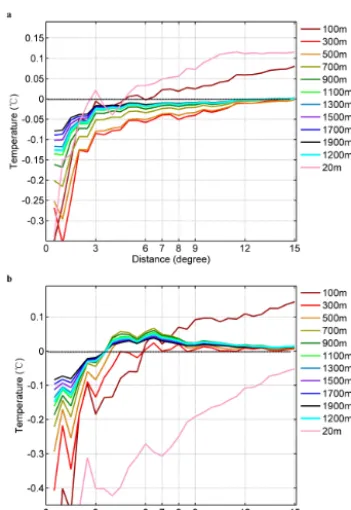
Figure 12. Column-averaged temperature anomalies within 4– 20 days after tropical cyclones, relative to pre-storm conditions, as a function of the horizontal box size across the storm track (from ±1◦to±15◦) for (a) TS/TD and (b) hurricanes. The colors are dif-ferent vertical sizes of the TC-affected box from 100 to 1900 m. The results for the box with 1200 m depth are highlighted in cyan.
relative to pre-storm conditions (Fig. 10), which is represen-tative of the ocean conditions in the restorative stage. Weak cooling still dominates the subsurface (100–200 m) response near the storm center. But, the standard error can be 100– 150 % of the signal, maybe because of the longer time win-dow (17 days in total). This weaker subsurface cold anomaly compared with the 0–3-day response implies that cooling caused by upwelling is being restored after storm passage, and this signal may be associated with the geostrophic ridge that develops in the wake of a storm following the disper-sion of near-inertial waves (Geisler, 1970). In addition, the near-surface cold anomaly along the right side of the storm is still apparent during this restoration stage, thus pointing to the persistence of the TC signal.
Figure 10 shows persistent warm anomalies between 20 and 200 m along both the right and left sides of the storm tracks, which are greater in magnitude than the observed forced stage response (0–3 days), with typical standard error (as a percentage of the TC signal) of 30–70 % for TS/TDs and 30–90 % for hurricanes. However, we do not find similar temperature anomaly structures in the background variabil-ity for high TC activvariabil-ity basins (e.g., western Pacific), even when extending the background pair selection criteria to 40 and 60 days.
b a
Figure 13. Two-hundred estimates (in cyan) of 0–1200 m column-averaged temperature as a function of distance across the storm track, based on randomly sampling 90 % of the Argo pairs for (a) TS/TD and (b) hurricanes, respectively. The mean and SDs are highlighted as the red line and error bars.
Figure 11 shows the vertical profile of the spatially aver-aged (−6 to+6◦) thermal response during the TC recovery stage relative to pre-storm conditions. We find that vertical mixing and upwelling/downwelling induces significant cool-ing near the surface (0–20 m depth) and subsurface warm-ing within the upper thermocline (50–200 m) for both TS/TD and hurricanes. The signals deeper than 200 m exhibit rela-tively weak cooling, and they are only significant for hurri-canes near the storm center. As noted by previous studies, deep ocean (below 400 m) thermal responses are rarely ob-served. One observation down to 530 m (Price, 1981) shows a large oscillation with amplitude about 30 m at the depth of 530 m after 10 days of storm passage. A study using a moor-ing observation (Brink, 1989) observed a TC-induced tem-perature oscillation at depths around 1000 m. Because of the lack of observations, further modeling and theoretical studies are needed to understand the response of the interior ocean to extreme surface wind forcing below 200 m.
3.4 Estimates of OHC changes after storm
stage. Temperature anomalies are plotted in Fig. 12 as a func-tion of the spatial and vertical extents of the TC footprint. Within 3◦of the storm center, both TS/TD and hurricanes in-duce column-averaged cooling at all depths. The cooling ef-fect decreases for increasing footprint size, approaching zero for TS/TD and a warming for hurricanes. This result suggests that upwelling and heat loss to the atmosphere near the storm center are partly (for TS/TD) or fully (for hurricanes) com-pensated by post-storm surface fluxes. Furthermore, when the footprint size is larger than 8–9◦, the absolute value of the average temperature anomalies decreases, which is again attributable to the “dilution” effect as discussed in the pre-vious section. The temperature anomalies also converge for increasing depth, when the footprint is greater than 3◦. Thus, we use a cross-track length scale of∼8◦and a depth scale of 1200 m to quantify the TC-induced upper ocean thermal re-sponse during the restorative stage. The average temperature anomalies for these footprint length scales are+0.039◦C for hurricanes and−0.0125◦C for TS/TD.
The annual contribution of the TC-induced OHC changes is calculated by multiplying the ocean temperature changes by yearly averaged track lengths. This method is based on our results that the averaged ocean thermal change over all storms between post-storm and pre-storm conditions is 0.039 and−0.0125◦C for hurricanes and TS/TD, respectively. The positive values indicate heat gained by the ocean. These es-timates correspond to a global annual flux contribution of ∼5.98 W m−2(0.75 PW) for hurricanes and∼ −1.90 W m−2 (−0.41 PW) for TS/TDs, where the positive values represent oceanic heat convergence.
Our results suggest that weak storms (TS/TD) tend to cool the ocean, while hurricanes tend to warm the ocean, when considering both storm-induced and post-storm fluxes. The difference in the ocean response may be due to the relatively weak vertical ocean mixing and surface cooling induced by TS/TD compared to hurricanes. For TS/TD, the OHC change is likely driven by the storm-induced enthalpy fluxes during passage. Because weaker storms typically cause less vertical mixing and thus less significant cold wakes following storms, there will be less post-storm heat flux into the ocean dur-ing the wake recovery stage. Conversely, strong events (hur-ricanes) induce more vertical mixing and surface cooling, which leads to more heat flux into the ocean during the re-covery stage and thus oceanic heat convergence. This finding supports previous results using altimetry (Mei et al., 2013) and simplified approaches based on sea-surface temperature changes (Sriver and Huber, 2007 and Jansen et al., 2010).
Similar to calculating the uncertainties of 0–3-day OHC change, the 200 estimates of TC-induced OHC changes are shown in Fig. 13. We choose the uncer-tainty to be equivalent to the SD of the average tem-perature change for spatial extent of 8◦ and 1200 m, consistent with the heat flux estimate. This uncertainty equates to ±0.0063◦C for TS/TD and ±0.0143◦C for hurricanes, which represents ∼50 % and 36 % of the
estimated OHC changes for TS/TD and hurricanes, re-spectively. Considering this uncertainty, our estimates of TC-induced thermal changes are −0.0125±0.0063◦C for TS/TD and 0.0390±0.0143◦C for hurricanes. Equivalently, these estimates correspond to global annual heat flux of −0.41±0.21 PW (−1.90±0.96 W m−2)for all TS/TD, and 0.75±0.25 PW (5.98±2.1 W m−2)for all hurricanes, where the positive values denote an oceanic heat convergence.
These findings indicate the total TC contribution to the global ocean heat convergence is estimated to be 0.34 PW annually in the 2004–2012 periods, which reflects an ocean heat gain from the atmosphere due to all storms.
4 Caveats
The methodology presented here contains several key caveats and limitations. One outstanding question relates to the accu-racy of the no-TC pairs in capturing the interannual variabil-ity in the timing of events. In other words, given that years with tropical cyclones are likely to have different position-ing/intensity of major atmospheric circulation patterns such as subtropical highs, one could expect to see a Rossby wave response from such shifts resulting in potentially anomalous trends at depth. To address this issue, we conducted the fol-lowing test.
TC-affected pairs are subdivided into two subsets: one contains data from 2004 to 2008 and the other from 2009 to 2012. We subdivide storms to analyze the sensitivity of our footprint results to different spatial patterns of storm lo-cations. The results for TS/TD and hurricane 4–20-day foot-prints are presented in Fig. 14, both compared with the 2004– 2012 results in black contours. In the figure, the main pattern is similar for the two time periods, with only some strength differences of the signals. In addition to this test, we calculate footprints of the background pairs for the two periods (not shown), and the differences are within the limit of insignif-icant noise. Results support the notion that the background signals can be mostly smoothed out by using a footprint strat-egy when averaging over large amounts of data with variant time and spatial distributions.
Figure 14. The 4–20-day averaged ocean thermal changes detected by using data from two year periods: 2004–2008 in the left panel and 2009–2012 in the right panel, shown in colors. The black con-tours are the result when using all of the data from 2004 to 2012, the same as the contours in Fig. 10. The results of hurricanes are pre-sented in the top panel and the bottom panel for TS/TD. The unit is◦C.
Ocean stratification varies regionally, which can in turn pose problems for estimating global averages of ocean re-sponses to TCs. To quantify the effect of regional variabil-ity, we calculate TC-induced ocean thermal changes within 4–20 days within three ocean basins separately: the Pacific Ocean, Indian Ocean and Atlantic Ocean. Note that we also subdivide the Pacific basin into separate regions – west-ern/eastern/southern Pacific). Figure 15 shows the results in the footprint composite format. Key findings include that (i) the global-averaged thermal footprint pattern (Fig. 10c) is generally consistent with the pattern in the Pacific Ocean, especially in the western Pacific (Fig. 15a, d), since there are ∼2500 pairs from the Pacific Ocean (or roughly∼60 % of the total number of pairs globally); and that (ii) although the footprints within the Atlantic and Indian oceans have large uncertainties, key characteristics of the general patterns are robust, such as ocean cooling near the storm center from the surface to subsurface (0–200 m) and subsurface warm-ing along both sides of the track (Fig. 15e, f). However, only 25 and 15 % of the Argo pairs globally are sampled from the Indian Ocean and Atlantic Ocean, respectively; thus, phys-ical interpretations are limited by the relative lack of data. In the eastern Pacific, the ocean responses seem to be differ-ent from other regions, which appears cooling at the left side of TCs as shown in Fig. 15b. This difference may be due to the lack of data in this region, indicating that our method is insufficient to reconstruct the local responses to TCs.
a
c
b
f d
e
Figure 15. Ocean thermal changes induced by hurricanes within 4–20 days after storm passage for individual ocean basins: (a) in the western Pacific Ocean, (b) in the eastern Pacific Ocean, (c) in the southern Pacific Ocean, (d) in the Pacific Ocean, (e) in the In-dian Ocean, and (f) in the Atlantic Ocean. The black contours are the global-averaged hurricane-induced ocean thermal changes in 4– 20 days, which are the same as those in Fig. 10c. The unit is◦C.
5 Conclusions
We use Argo data to create a global representation of TC-induced changes in upper ocean temperature, using a new footprint method to create a composite analysis of the ver-tical profile of the cross-track ocean temperature response for two distinct timescales (0–3 and 4–20 days relative to storm passage) and categories (TS/TD and hurricanes). We find this method is capable of capturing the main character-istics of TC-induced ocean variability related to cross-track and intensity variations, as well as the differences in the re-sponse due to the choice of timescales (e.g., forcing versus recovery).
uncer-b a
Figure 16. (a): the annual TC-induced ocean heat loss via air–sea heat flux in 0–3 days (blue line) and the ocean heat content changes after storms (in 4–20 days) (red line). The positive values show the ocean heat gain. The linear trend of the ocean heat gain is presented in pink, and the trend is 0.046×10²²J yr−1. (b): yearly averaged track lengths for both TS/TD (blue) and hurricanes (in red).
tainty of our estimate is about 20 % for TS/TD and 25 % for hurricanes.
Recent in situ, remotely sensed and reanalyzed air–sea heat flux products (Smith et al., 2011) have faced challenges in closing the ocean heat budget. These analyses show a global oceanic heat gain of 20–30 W m−2(Josey et al., 1999), while the global mean heat flux is ∼0.5 W m−2 from ob-served variations in OHC. Our observational results suggest that TCs may provide a potential mechanism (heat flux in a high wind regime) for filling this gap.
After storm passage, ocean conditions in TC-affected gions experience a recovery process to at least partially re-store upper-ocean conditions pre-storm or climatological val-ues through enhanced air–sea fluxes leading to ocean heat convergence. This recovery stage lasts much longer than the forcing stage during the storm passage. We estimate the changes in a timescale of 4–20 days relative to pre-storm conditions, which implicitly includes fluxes during the forced stage. On this timescale, around ∼0.75 PW (5.98 W m−2)
of heat is transferred annually from the atmosphere to the ocean for hurricanes, which represents an ocean heat gain after storms. However, TS/TD exhibit an opposite response,
∼ −0.41 PW (1.90 W m−2), representing an ocean heat loss for weaker events. We estimate the uncertainty to be about 50 % of our estimates for TS/TD and 35 % for hurricanes. The opposite sign of OHC changes after storm (4–20 days) for weak and strong storms implies that the impact of these events on the upper ocean is sensitive to the intensity. This result also suggests that additional atmospheric heating due to anthropogenic warming may potentially increase the rate of TC-induced ocean heat uptake, since research suggests the number of strong TCs may increase with continued warming (Bender et al., 2010; Knutson et al., 2010).
To assess the TC contribution to historical trends in the ocean heat uptake, we calculate the total air–sea heat flux in each year from 1970 to 2010, by assuming that each TS/TD transfers 6.25 W m−2 and each hurricane transfers 4.8 W m−2 heat from the TC-affected region to the atmo-sphere during 0–3 days after storm. The annual heat flux is shown in Fig. 16 in blue. The figure shows a maximum at-mospheric heating of∼12×1022J during 1996∼1997 and a generally larger signal between 1988 and 1998, which is due to more TC activity during these years. As suggested in Trenberth and Fasullo (2007), the El Niño activity during these years (three between 1990 and 1995 and a large event in 1997–1998) may be at least partially responsible for this boost of TC activity in the western Pacific.
Figure 16 also shows the accumulated TC-induced OHC changes in recovery stages (4–20 days) relative to pre-storm conditions. We assume the OHC change is −1.9 W m−2 for TS/TD and 5.98 W m−2 for hurricanes (a positive value shows a heat gain by the ocean). OHC changes show that TC-induced ocean heat convergence has been increasing since 1970. This OHC change is likely due to the increase in the fraction of strong storms during the past 40 years (Knutson et al., 2010). The linear trend of TC-induced ocean heat uptake is about 0.046×10²²J yr−1, which is 11 % of global ocean heat uptake of the uppermost 2000 m during the past 55 years (∼0.42×10²²J yr−1) (Levitus et al., 2012).
Appendix A: The composite footprint method
As discussed in Sect. 2.2, we introduce a footprint method that averages all of the TC-induced cross-track (i.e., perpen-dicular to the storm’s direction of motion) ocean temperature changes. We define TC-induced ocean thermal changes cal-culated from Argo pairs using the functional form
dTa1=dTa1(ID,dist,track,depth, δt ),
where ID identifies the particular storm, dist is the distance between the observation location and the track center perpen-dicular to the storm’s direction of motion (the cross-track dis-tance in the storm coordinate system), track denotes the spa-tial location of an Argo pair related to a TC track (the along-track distance in the storm coordinate system), depth denotes the vertical depth of the temperature anomalies, and δt is the time difference between the observing time of the TC-affected Argo profile and the time of the nearest track center. We define the positive values of dist to be consistent with the asymmetric inertial response (to the right in the North-ern Hemisphere and to the left in the SouthNorth-ern Hemisphere), referred to as TC-track coordinates (Price et al., 2008).
To create a composite representation of the average ocean response, we reduce the five-dimensional function dTa1to a three-dimensional function by averaging the anomalies over all TC conditions corresponding to two predefined categories (TS/TD and hurricanes). We define a track-averaged foot-print of ocean thermal changes over all tracks, and we sepa-rate the events into two distinct categories: TS/TD and hurri-canes. Track locations with maximum wind speeds less than 63 knots are categorized as TS/TD, and all others are catego-rized as hurricanes (this hurricane category represents con-ditions when a TC is in hurricane status). The footprint is represented as
FTSTD(dist,depth, δt )=
ID=nTSTD
X
ID=1
dTa1(ID,dist,track,depth, δt )dtrack
nTSTD(dist,depth, δt ),
FHur(dist,depth, δt )=
ID=nHur
X
ID=1
dTa1(ID, dist, track, depth, δt )dtrack
nHur(dist,depth, δt ).
In these equations, the dTa is the observational
temper-ature anomaly. The number of the tempertemper-ature anomalies at each dist, depth and δt is denoted as nTSTDandnHurfor TS/TD and hurricanes, respectively.
We construct the three-dimensional footprints by grouping temperature anomalies from TS/TD and hurricanes, respec-tively, with dimensions dist containing 0.5◦bins from−8 to +8◦across the track,δt containing 0.5-day bins from 0 to 20 days, and depth containing 10 m bins from 5 to 1000 m and 50 m bins from 1000 to 2000 m. In each grid box, av-erages of the temperature anomalies are calculated by using temperature anomalies from this box and 14 other adjacent
Figure A1. Tracks of tropical cyclones from January 2004 to De-cember 2012, associated with the distribution of Argo pairs used in the paper. The colors of the tracks indicate the categories of tropical cyclone–tropical depression (TD; yellow), tropical storm (TS; or-ange), and category 1–5 cyclones (denoted by red, magenta, purple, blue, and black from categories 1 to 5, respectively). The locations of Argo pairs are dotted in two colors: cyan dots are the pairs lo-cated at the right side of the corresponding TC track, and green dots are the pairs located on the left side of the track. We analyze 885 tracks and a total of 4410 Argo pairs.
bin boxes (in time and dist, dimensions between−0.5 and 0.5 days, and−1 to 1◦relative to the given box).
We use this strategy to capture the main variability of the ocean response and to avoid potential biasing caused by the uneven distribution of Argo pairs in space and time. Key points of this methodology include (1) categorizing the events into weak and strong events/conditions, and (2) focus-ing on the cross-track temperature response, usfocus-ing a footprint technique that neglects along-track variability. Point (2) re-flects the assumption about the importance of the asymmetric cross-track thermal response compared to along-track direc-tions, which has been noted in numerous previous case stud-ies (Black and Dickey, 2008; Deal, 2011; Price et al., 2008). However, recent studies (Jaimes and Shay, 2010; James et al., 2011) suggest ocean variability along the track can sub-stantially modulate the ocean cooling response to TC forc-ing and distort the temperature anomaly in the wake of the storm, which can be important within western boundary cur-rents and associated geostrophic vortices. As a first step to determining TC effects on upper ocean thermal structure on a global scale, we focus primarily on the cross-track ocean response.
As stated previously, our methodology requires the dis-tance between two Argo profiles in a pair to be less than 0.2◦. However, we do not require the pre-storm and post-storm measurements to be recorded from the same float. This criterion is in contrast to recent regional analysis using Argo data (Park et al., 2011), which stipulated the constraints that two profiles are to be measured by the same Argo float in order to reduce the float-to-float calibration difference, and the maximum distance between measurements is to be less than 200 km. In the current study,∼80 % of the pre-storm and post-storm measurements are from the same float.
Figure A2. Locations of TC-affected Argo pairs with colors show-ing the cross-track distances of their locations relative to the cor-responding storm track. Positive values indicate pairs to the right (left) side of the track in the Northern Hemisphere (Southern Hemi-sphere).
Figure A3. Histograms of the Argo float pairs for different statis-tics: (a) storm category, (b) time after storm passage (0.5-day bin), (c) distance from the storm center (0.5◦bin), and (d) depth (10 m bin). In (c), a positive distance represents the right (left) side of the track in the Northern Hemisphere (Southern Hemisphere), and a negative distance represents the left (right) side in the Southern Hemisphere (Northern Hemisphere).
to December 2012, highlighting the global coverage of the Argo pairs in TC-affected regions (4410 total pairs). Tropi-cal cyclones have preferred locations and directions of mo-tion. For example, TCs in the northwestern Pacific move to the northwest between 10 and 20◦N and northeast between 20 and 40◦N. This preferred storm location and direction of motion result in coastal pairs in the northwestern Pacific located on the left side of the tracks, while the pairs away from the coast are typically located on the right side of the tracks. In the northeastern Pacific, TCs generally move to the northwest, leading to a clear distribution of right-side pairs in 20–40◦N and left-side pairs in 0–20◦N. Similarly, in the northern Atlantic, the distribution of TCs leads to the left-side pairs mainly being distributed between 0–15 and 40– 50◦N. But, in the Indian and southern Pacific oceans, the left- and right-side pairs mix together. These preferred lo-cations of TCs and the resulting distributions of Argo pairs (Fig. A2) can affect the geographical patterns of the TC-induced oceanic response.
The distributions of Argo pairs are presented in Fig. A3 for the category, observation time (relative to storm pas-sage), depth, and distance from storm center. Fig. A3 reflects several key features of the methods and analysis, including (1) the uneven distribution of the data and (2) the larger num-ber of Argo pairs for the TS/TD conditions than for hurri-canes (TS/TD conditions are much more common). (3) The
number of Argo pairs decreases with time (e.g., we sample more pairs between 0 and 10 days after storm passage com-pared to between 10 and 20 days). (4) We obtain the least number of pairs near storm centers. Point (4) may be due, in part, to unreliable Argo measurements associated with severe conditions near storm centers (bad profiles) and/or strong horizontal currents (∼100 cm s−1) advecting the floats away from the storm centers. To check whether there are some systematic differences (i.e., drifting) in horizontal distance between the two profiles in a pair, we calculate the horizon-tal difference between the two profiles as in Appendix D. In both geographical coordinates and track coordinates, we find no significant effects of drifting.
Appendix B: Estimation of background variability in Argo pairs
Isolating the TC-induced thermal changes using Argo floats is difficult, because biases can arise due to changes in the thermal structure of the background ocean state. These bi-ases can be caused by many processes such as the seasonal cycle, meso-scale signals and large-scale spatial variability. Here we employ a test to examine potential biases and quan-tify background errors related to our footprint method de-scribed in the previous sections. Background noise is esti-mated by using Argo pairs under quiescent conditions (i.e., without TCs), hereafter denoted as NoTC pairs.
Our methodology for analyzing background variability is outlined in the following steps.
1. We collect all Argo profiles during January 2004– December 2012 for which there are no TCs within±8◦ distance of their location and−50 to +5 days relative to storm passage. These profiles are denoted as NoTC profiles.
2. Background Argo pairs are formed by using these NoTC profiles. The sampling strategy is the same as the TC pairs. One Argo pair consists of two Argo pro-files, which are within 0.2◦and 20 days. Twenty days is set here to make this timescale comparable with the timescale of the typical TC response. We tested the sen-sitivity of the analysis to the choice of timescale by also analyzing variability out to 40 days. The results were consistent for both timescales.
collected across all years corresponding to storm track locations and timing of events (within a given year). This sampling strategy provides a consistent method for analyzing background variability, by comparing Argo pairs from the same regions and times of year during storm (TC pairs) and non-storm (NoTC pairs) condi-tions.
4. To frame the background signals into the context of our footprint method, the NoTC pairs obtained in step (3) are converted to a background footprint (denoted as the NoTC-TSTD footprint and the NoTC-Hur foot-print for TS/TD and hurricanes, respectively). To sum-marize the method, each TC footprint bin, for exam-pleFTSTDwith a bin denoted by (dist, depth,δt ), con-tainsnTC-affected pairs with geographical locations of (lati, loni) i=1 :n. The NoTC-TSTD footprint
(NoTC-Hur footprint) at the same bin (dist, depth, δt )is cal-culated by selecting m NoTC pairs according to the locations of TC-affected pairs. If there exists a NoTC pair within 2◦to (lati, loni), this NoTC pair is selected
to calculate the NoTC-TSTD footprint (dist, depth,δt )
(NoTC-Hur footprint (dist, depth,δt )). In the construc-tion of the background footprint,mis set ton. In this case, we define background variability at a single loca-tion in terms of one NoTC pair. Using one NoTC pair corresponding to a given TC pair enables strict compar-ison between the two data sets. Otherwise, the method will yield more weight to individual pairs from loca-tions with low TC activity (e.g., where there are many NoTC pairs compared to TC pairs). However, we have performed additional tests using all of the pairs from step (3), and the results are generally consistent with the constraints employed here.
By using the background pairs selected as above, both the NoTC-TSTD footprint and NoTC-Hur footprint are obtained according to the footprint method proposed in the previous section. In this case, the background signals can be directly comparable to the TC footprint (FTSTDandFHur).
In total, 13 701 pairs are collected after step (3) is ducted. All the Argo profiles are under the same quality con-trol procedures as the TC-affected Argo profiles discussed in the previous section. Figure B1a and b display the total num-ber of TC pairs and NoTC pairs in each 4◦ by 8◦grid box. The spatial distribution of NoTC pairs is generally consistent with the TC-affected pairs.
The errors and biases due to the presence of background variability are quantified using two independent methods de-scribed in the following subsections. We first conduct a gross check on background error, and we quantify the background error using the footprint method.
a
b
Figure B1. Counts of the (a) NoTC pairs and (c) TC-affected pairs in each 4◦by 8◦grid box.
B1 Gross check
By applying a gross check, we are aiming to check the mag-nitude of the global-averaged background signals and the size of the background uncertainties in TC-affected regions and seasons. We also compare the error with a standard Argo accuracy of ∼0.005◦C. We define the temperature differ-ences of these NoTC pairs as background noise (dBTa)using
the functional form
dBTa=dBTa(time, δt,depth, lat, lon),
where time denotes the Julian day of the reference Argo pro-file;δt is the time difference between the two Argo profiles in each pair; lat and lon denote the spatial locations of a pair; and depth is the depth of a temperature anomaly. These anomalies are collected in two maps to test for any systemat-ical temporal or spatial biases in background pairs:
Back-Map1(depth)=
day2
Z
day1 δtn Z
δt1 lat2 Z
lat1 lon2 Z
lon1
dTa1(day, δt,depth, lat, lon)dlondlatdδtdday/n(depth),
Back-Map2(δt )=
day2
Z
day1
depthn
Z
depth1
lat2 Z
lat1 lon2 Z
lon1
dTa1(day, δt,depth, lat, lon)dlondlatddepthdday/n(δt ).
where n(depth) and n(δt ) denote the number of pairs for each depth and eachδt, respectively. In Back-Map1, all of the background temperature anomalies are grouped into bins representing 5 m thickness between 0 and 2000 m in depth. In Back-Map2, temperature anomalies are grouped into tem-poral bins of size 0.5 days between 0 and 20 days.
a
b
b
a
Figure B2. Background ocean temperature variability as a function of depth and time. (a) Mean (green curve) and 1 SD (green shading) of background variability as a function of depth, compared with 1 SD of hurricane and TS/TD affected pairs. (b) Time evolution of background variability of 0–1000 m average (light green line and light green shading for mean and SD, respectively). The SDs of temperature anomalies in Argo pairs under TS/TD and hurricane conditions are plotted in light blue and light red, respectively.
by seasonal/meso-scale signals. However, this anomaly is negligible compared to TC signals (discussed in the follow-ing sections).
The means of the background variability as a function of time also show no trend with δt (Fig. B2b) for 0–1000 m (also no trend for 0–20 m; not shown here). The 0–1000 m averaged SDs of Argo pairs influenced by hurricanes and TS/TD show a 0.1–0.2◦C larger deviation compared to es-timates of background variability, which shows that TCs can disturb normal ocean conditions and that the perturbation is observable using this methodological framework.
Next, we apply a bootstrap analysis to determine the effect of sample size on characterizing potential biases, errors, and background variability. At each depth, we randomly choose a certain number of pairs (the number of samples changes from 10 to 9000, with a step size of 20), and we calculate the mean of the temperature anomalies of the chosen pairs. This procedure is repeated 200 times yielding 200 means, and we calculate the SD of the 200 means at each vertical level. Figure B3a shows the standard error at different depths against sample sizes, indicating that the error of the
temper-b
b
a a
b
a
Figure B3. Bootstrap analyses of background noise. (a) Standard errors at different depth versus sample numbers with colors denot-ing different depths. (b) Standard errors at different times versus sample numbers with colors denoting different times. Solid lines are the results from using the whole NoTC pairs data set, and the dots show the same results for the TC-affected pairs.
ature anomalies decreases with sample size. When sample sizes are greater than 400, the standard error at depths deeper than 400 m is less than 0.02◦C, and at depths less than 400 m, the standard error is less than 0.06◦C. Both of these errors are less than 5 % of SDs at corresponding depths shown in Fig. B3a. When the sample size is increased, the error is grad-ually reduced and converges near the Argo sensor accuracy (0.005◦C) for the upper shallow depths and below the Argo sensor accuracy for deeper levels. This result suggests that increasing the amount of data generally reduces the back-ground error when averaged over large areas.