Small world in a seismic network: the California case

(1)

www.nonlin-processes-geophys.net/15/389/2008/ © Author(s) 2008. This work is distributed under the Creative Commons Attribution 3.0 License.

Nonlinear Processes

in Geophysics

Small world in a seismic network: the California case

A. Jim´enez1, K. F. Tiampo1, and A. M. Posadas2

1_{Department of Earth Sciences Biological and Geological Sciences, University of Western Ontario, London, Canada} 2_{Department of Applied Physics, University of Almer´ıa, Almer´ıa, Spain}

Received: 31 January 2008 – Revised: 4 April 2008 – Accepted: 5 April 2008 – Published: 9 May 2008

Abstract. Recent work has shown that disparate systems can be described as complex networks i.e. assemblies of nodes and links with nontrivial topological properties. Examples include technological, biological and social systems. Among them, earthquakes have been studied from this perspective. In the present work, we divide the Southern California re-gion into cells of 0.1◦, and calculate the correlation of activ-ity between them to create functional networks for that seis-mic area, in the same way that the brain activity is studied from the complex network perspective. We found that the network shows small world features.

1 Introduction

Physics, a major beneficiary of reductionism, has developed an arsenal of successful tools to predict the behavior of a sys-tem as a whole from the properties of its constituents. The success of these modeling efforts is based on the simplicity of the interactions between the elements: there is no ambigu-ity as to what interacts with what, and the interaction strength is uniquely determined by the physical distance. We are at a loss, however, in describing systems for which physical dis-tance is irrelevant, or there is ambiguity whether two compo-nents interact (Albert and Barab´asi, 2002).

Historically, the study of networks has been mainly the domain of a branch of discrete mathematics known as graph theory. Since its birth in 1736, when the Swiss mathemati-cian Leonhard Euler published the solution to the K¨onigsberg bridge problem (consisting in finding a round trip that tra-versed each of the bridges of the Prussian city of K¨onigsberg exactly once), graph theory has witnessed many exciting de-velopments and has provided answers to a series of practi-cal questions such as: what is the maximum flow per unit

Correspondence to: A. Jim´enez

([email protected])

time from source to sink in a network of pipes, how to color the regions of a map using the minimum number of colors so that neighboring regions receive different colors, or how to fill n jobs by n people with maximum total utility. In addition to the developments in mathematical graph theory, the study of networks has seen important achievements in some specialized contexts, as for instance in the social sci-ences. Social networks analysis started to develop in the early 1920s and focuses on relationships among social en-tities such as communication between members of a group, trades among nations, or economic transactions between cor-porations (Boccaletti et al., 2006).

Recent work has shown that disparate systems can be de-scribed as complex networks, that is, assemblies of nodes and links with nontrivial topological properties, examples of which include technological, biological and social systems (Egu´ıluz et al., 2005). Among them, earthquakes also have been studied from this perspective (Abe and Suzuki, 2004, 2006a; Baiesi and Paczuski, 2005). In the past few years, the discovery of small-world and scale-free properties of many natural and artificial complex networks has stimulated a great deal of interest in studying the underlying organizing princi-ples of various complex networks, and has led to dramatic advances in this emerging and active field of research (Wang and Chen, 2003). Here we present for earthquake fault sys-tems a similar approach to that of Egu´ıluz et al. (2005) for functional brain networks, and find that the analyzed catalog has small-world behavior.

(2)

390 A. Jim´enez et al.: Small world seismic network

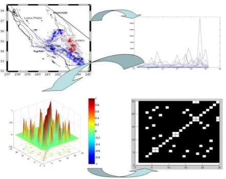
Fig. 1. Scheme of the method.

Strogatz (1998), in their seminal paper, have proposed to de-fine small-world networks as those networks having both a small value ofLp (characteristic path length), like random graphs, and a high clustering coefficientC, like regular lat-tices. They consider a one-dimensional graph withN nodes, each vertex being connected to itsknearest neighbors (where N kln[N]). The numberkof edges per vertex is also called the degree of the graph. Next, with a probabilityP, a random edge is chosen and rewired to connect to a randomly chosen vertex. By varyingP between 0 and 1 graphs can be created which span the whole range from regular (P=0) to random (P=1).

Two measures were introduced to characterize such graphs: the characteristic path lengthLpis the mean of the shortest path (expressed in number of edges) connecting any two vertices on the graph. The cluster coefficientCpis the likelihood (between 0 and 1) that thekvneighbors of vertex vare also connected to each other, averaged over all vertices. Regular networks or graphs have a highCp(Cp≈3/4) but a long characteristic path length (Lp≈N/2k); random graphs have a lowCp(k/N ) but the shortest possible path length (Lp≈ln(N )/ ln(k)). The discovery of Watts and Strogatz was that some networks with 0<P1, thus regular networks with only a very small number of random edges, have a path length that is much smaller than that of a regular network, while theCpis still close to that of a regular network. This dramatic drop inLp for P only slightly higher than 0 im-plies that any vertex on the graph can be reached from any other vertex in only a small number of steps. This is equiv-alent to the small-world phenomenon and this type of graph (Cpclose to regular network;Lpclose to random network) was called a small-world graph by Watts and Strogatz. They showed that many real world networks such as networks of actors playing in the same movies, the power grid of North America, and the neuronal network of Caenorhabditis

ele-gans have small-world features. Furthermore, they suggested

that such networks may be optimal for information process-ing in complex systems. Since then it has been shown that many real networks display small world features and that these may reflect an optimal architecture for information pro-cessing (Stam, 2004).

2 Method

For a network (or graph) representation, first we have to de-fine the nodes and the edges. Figure 1 shows a scheme of the method. The seismic region is divided into squared cells (for latitude and longitude only in this particular case), which will be the nodes; the time is divided into intervals. At each time step (we will try some, from days to several years), the ac-tivity,a(x, t )of the cell is calculated as the number of earth-quakes at that cell and time. Now we have a time series for each cell. For each pair of cells,x1 andx2, we calculate their correlation coefficient in this way:

r(x1, x2)= ha(x1, t )a(x2, t )i − ha(x1, t )i ha(x2, t )i

σ (a(x1))σ (a(x2)) (1)

whereσ2(a(x))=a(x, t )2− ha(x, t )i2, andh·i represents temporal averages.

Then, a threshold matrix is calculated for different values of the correlation coefficient,rc, so that when the correlation

between two cells (nodes) is higher than the threshold value (positive values ofrc only), we say that they are positively

correlated, and the nodes (cells) are connected by an edge. Once our network is defined, we proceed to analyze its prop-erties.

2.1 Node degree and degree distributions

The degree (or connectivity)di of a nodeiis the number of

edges incident with the node, and is defined in terms of the adjacency matrixAas:

di = N X

j=1

aij (2)

The most basic topological characterization of a graph can be obtained in terms of the degree distributionp(d), defined as the probability that a node chosen uniformly at random has degreed or, equivalently, as the fraction of nodes in the graph having degreed.

2.2 Shortest path lengths and diameter

The shortest path is the geodesic distance between vertex pairs in a network. The mean geodesiclis then:

l= 1

1

2n(n+1) X

i≥j

gij (3)

wheregij is the geodesic distance from vertex i to vertex

(3)

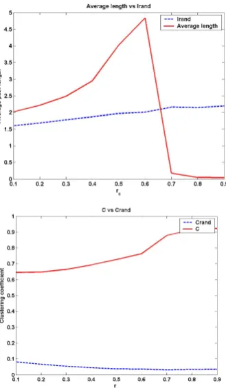
Fig. 2. Average length and clustering coefficient of the networks

with different thresholds (rc) compared to those corresponding to a

random graph with the same number of nodes and the same average node degree, for time lags of 1 day.

gij is called the diameter of the graph. We used Dijkstra’s

algorithm to implement this calculation (Dijkstra, 1959). 2.3 Clustering

A clear deviation from the behavior of the random graph can be seen in the property of network transitivity, sometimes also called clustering (Newman, 2003). Here we use the def-inition by (Watts and Strogatz, 1998), that has found wide use in numerical studies and data analysis (Newman, 2003):

C= 1 n

X

i

Ci (4)

Ci =

number of triangles connected to vertex i

number of triples centered on vertex i (5)

where triple means a single vertex with edges running to an unordered pair of others. The clustering coefficient measures the average density of triangles in a network. For random networks,Ctends to zero asn−1in the limit of large system size.

random graph with the same number of nodes and the same average node degree, for time lags of 100 days.

3 Data

The catalog belongs to the Southern California Earthquake Center (SCEC) and contains the seismic data for the period 1 January 1984 to 3 July 2001. The analyzed area ranges from 32–37 N, and 115–121 W. The magnitude spans from 3.0 to 8.0. The catalog is complete above magnitude 3.

(4)

random graph with the same number of nodes and the same average node degree, for time lags of 1000 days.

4 Results

As can be seen in Figs. 2–4, the clustering coefficient for the connected components is always much higher than that of a random network. It also shows that for correlations be-tween the cells higher than 0.8, the average path is always lower than that of a random network. So, when we apply a threshold forrc higher than that 0.8, we obtain a complex

network which behaves as a small world, as defined in (Watts and Strogatz, 1998). Note that we are interested in study-ing highly correlated cells, andrc>0.8 is therefore a good

lower threshold for our seismicity network. Note also that the thresholdrc affects the connectivity of generated networks.

Largerrcwill result in the disconnected network whose

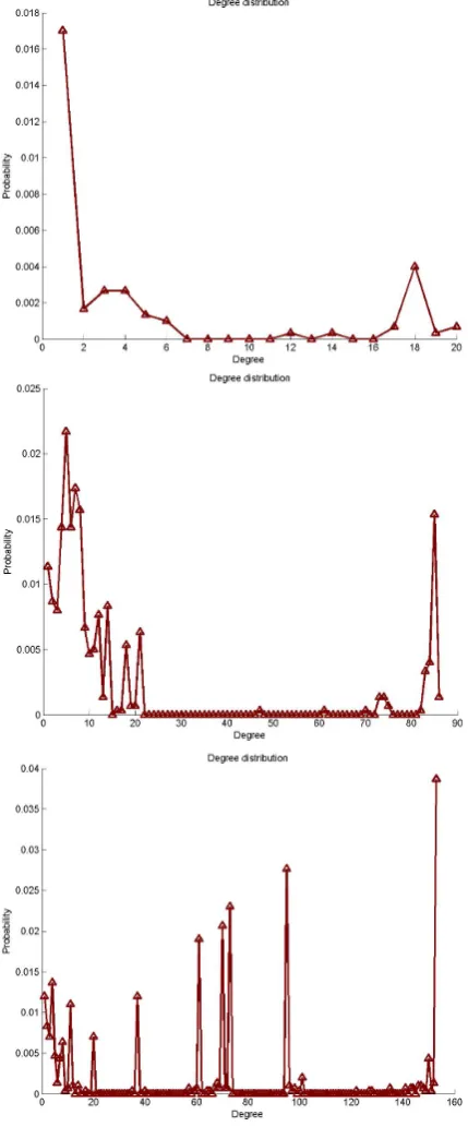
av-erage short path length will become very large in the sense of graph theory, which would be different from the results in the figures. In Fig. 5 we show the degree distribution for rc=0.8 and 1, 100, and 1000 days, respectively. They are not

scale free. This result is opposite to that found previously in (Abe and Suzuki, 2004, 2006a; Baiesi and Paczuski, 2005). Thus, the scale invariance is violated by thresholding. This implies that thresholding eliminates an important element of complexity of a seismic network. We also analyze the scaling relationship between the clustering coefficient and the degree

Fig. 5. Degre distribution forrc=0.8 and 1 day, 100 days, 1000 days

lag, respectively. As can be seen, they are not scale free.

(Abe and Suzuki, 2006b). We see that it is also violated by thresholding (Fig. 6).

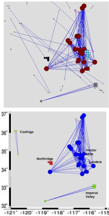
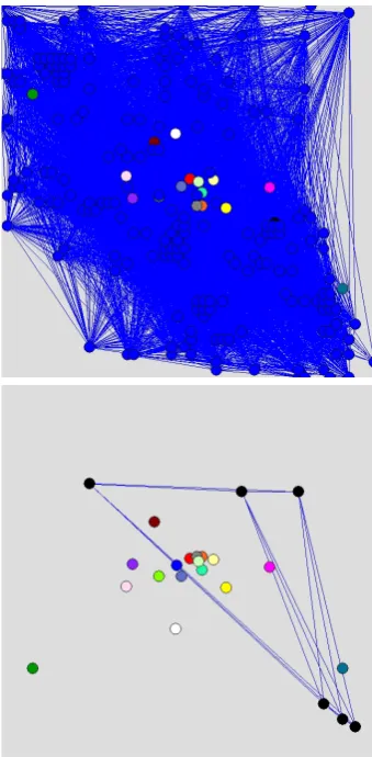
In Fig. 7 we present the networks obtained withrc>0.8

(5)

Fig. 6. Clustering in function of the degre forrc=0.8 and 1 day,

100 days, 1000 days lag, respectively. As can be seen, they are not scale free.

is interesting to note that those Coalinga and Imperial Valley earthquakes have cells relatively far from them, but with a high correlation in the seismicity rate series.

When we visualize the network for 100 days lag, we can see that there are much more main components (56) than be-fore (6) by using the hierarchical algorithm. The main

com-Fig. 7. Networks obtained forrc>0.8, by using a betweenness and a hierarchical algorithm (with some of the main earthquakes in the region) to find the components, with Pajek (Batagelj and Mrvar, 1998), for time lags of 1 day.

ponent (first in Fig. 8) is the same as the main component for 1 day lag. Other particular components are related to differ-ent earthquakes. Most of the clusters’ links outline clearly the San Andreas fault direction.

The number of clusters decreases with respect to the net-work found for the 100 days lag. In Fig. 9, the main compo-nent for the 1000 days lag relates the whole area.

(6)

Fig. 8. Some of the 56 components for the 100 days time interval

andrc>0.8, by using a hierarchical algorithm to find the compo-nents, with Pajek (Batagelj and Mrvar, 1998).

distant nodes. However, as can be deduced from the net-works for 1 day lag (Fig. 7), there are some long range links, in particular following the San Andreas fault. Since the rate of earthquakes is related to the stress transfer (Helmstetter et al., 2005), the networks reflect the way stresses are diffused in the area.

Fig. 9. Some of the 18 components for the 1000 days time interval

andrc>0.8, by using a hierarchical algorithm to find the

compo-nents, with Pajek (Batagelj and Mrvar, 1998).

5 Conclusions

We propose a different analysis of seismicity in terms of complex networks. They are obtained in a way similar to the way brain functional networks are studied (Egu´ıluz et al., 2005). In our preliminary results, we see that the dif-ferent components of the obtained networks act as difdif-ferent responses to the stimulus given by the general plate motions in the region. The results of this study show that the func-tional connectivity matrix of seismic activity recordings can be converted into a sparsely connected graph by applying a suitable threshold ofrc. So, it can be said that the highest

(7)

earthquake activities. Another choice would be to let these “small-world” networks to be weighted. In the present study we only made our analysis in two dimensions, due to limita-tions in the computalimita-tions.

Acknowledgements. This work was partially supported by the

MCYT project CGL2005-05500-C02-02/BTE, the MCYT project CGL2005-04541-C03-03/BTE, and the Research Group “Geof´ısica Aplicada” RNM194 (Universidad de Almer´ıa, España) belonging to the Junta de Andaluc´ıa. The work of K. F. Tiampo was funded under the NSERC and Benfield/ICLR Industrial Research Chair in Earthquake Hazard Assessment. The work of A. Jiménez was funded by a “Fundación Ramón Areces” Grant.

Edited by: J. Kurths

Reviewed by: two anonymous referees

References

Abe, S. and Suzuki, N.: Scale-free network of earthquakes, Euro-phys. Lett., 65, 4, 581–586, 2004.

Abe, S. and Suzuki, N.: Complex-network description of seismicity, Nonlin. Processes Geophys., 13, 145–150, 2006,

http://www.nonlin-processes-geophys.net/13/145/2006/. Abe, S. and Suzuki, N.: Complex earthquake networks:

Hierar-chical organization and assortative mixing, Phys. Rev. E., 74, 026113, 2006.

Albert, R. and Barab´asi, A. L.: Statistical mechanics of complex networks, Rev. Mod. Phys., 74, 47–97, 2002.

Baiesi, M., Paczuski, M.: Complex networks of earthquakes and aftershocks, Nonlin. Processes Geophys., 12, 1–11, 2005, http://www.nonlin-processes-geophys.net/12/1/2005/.

Batagelj, V. and Mrvar, A.: Pajek – program for large network anal-ysis, Connections, 21, 47–57, 1998.

Boccaletti, S., Latora, V., Moreno, Y., Chavez, M., and Hwang, D. U.: Complex networks: Structure and dynamics, Physics Re-ports, 424, 175–308, 2006.

Dieterich, J.: A constitutive law for rate of earthquake production and its application to earthquake clustering, J. Geophys. Res., 99, 2601–2618, 1994.

Dijkstra, E. W.: A note on two problems in connection with graphs, Numerische Math., 1, 269–271, 1959.

Egu´ıluz, V. M., Chialvo, D. R., Cecchi, G. A., Baliki, M., and Ap-karian, A. V.: Scale-free brain functional networks, Phys. Rev. Lett., 94, 018 102–018 104, 2005.

Helmstetter, A., Kagan, Y. Y., and Jackson, D. D.: Importance of small earthquakes for stress transfers and earthquake triggering, J. Geophys. Res., 110, doi:10.1029/2004JB003286, B05S08, 2005.

Kochen, M.: The Small World, Ablex, Norwood 1989.

Milgram, S.: The small world problem, Physch. Today, 2, 60–67, 1967.

Newman, M. E. J.: The structure and function of complex networks, SIAM Review, 45, 2, 167–256, 2003.

Southern California Earthquake Center: available at http://www. data.scec.org/.

Stam, C. J.: Functional connectivity patterns of human magnetoen-cephalographic recordings: a “small-world” network?, Neuro-science Lett., 355, 25–28, 2004.

Wang, X. F. and Chen, G.: Complex networks: small-world, scale-free and beyond, IEEE Circuits and Systems Magazine, 3, 6–20, 2003.