www.nonlin-processes-geophys.net/15/145/2008/ © Author(s) 2008. This work is licensed
under a Creative Commons License.
Nonlinear Processes
in Geophysics
Multivariate analysis of nonlinearity in sandbar behavior
L. Pape and B. G. Ruessink
Department of Physical Geography, Faculty of Geosciences, IMAU, Utrecht University, P.O. Box 80.115, 3508 TC Utrecht, The Netherlands
Received: 13 September 2007 – Revised: 30 November 2007 – Accepted: 8 January 2008 – Published: 18 February 2008
Abstract. Alongshore sandbars are often present in the nearshore zones of storm-dominated micro- to mesotidal coasts. Sandbar migration is the result of a large num-ber of small-scale physical processes that are generated by the incoming waves and the interaction between the wave-generated processes and the morphology. The presence of nonlinearity in a sandbar system is an important factor de-termining its predictability. However, not all nonlineari-ties in the underlying system are equally expressed in the time-series of sandbar observations. Detecting the presence of nonlinearity in sandbar data is complicated by the de-pendence of sandbar migration on the external wave forc-ings. Here, a method for detecting nonlinearity in multi-variate time-series data is introduced that can reveal the non-linear nature of the dependencies between system state and forcing variables. First, this method is applied to four syn-thetic datasets to demonstrate its ability to qualify nonlin-earity for all possible combinations of linear and nonlinear relations between two variables. Next, the method is applied to three sandbar datasets consisting of daily-observed cross-shore sandbar positions and hydrodynamic forcings, span-ning between 5 and 9 years. Our analysis reveals the presence of nonlinearity in the time-series of sandbar and wave data, and the relative importance of nonlinearity for each variable. The relation between the results of each sandbar case and pat-terns in bar behavior are discussed, together with the effects of noise. The small effect of nonlinearity implies that long-term prediction of sandbar positions based on wave forcings might not require sophisticated nonlinear models.
1 Introduction
Sandbars are alongshore ridges of sand in up to 10 m water depth along micro- to mesotidal, storm-dominated coasts and strongly affect the nearshore flow field and sediment trans-port processes. They continuously change their position in Correspondence to: L. Pape
(l.pape@geo.uu.nl)
response to temporal variability in the offshore wave forcing. During storms intense wave breaking drives strong offshore-directed currents that force the sandbar offshore (e.g. Gal-lagher et al., 1998). Wave nonlinearity (preponderance of high crests and steep front faces) drives onshore migration during intermediate and low-energy conditions (Hoefel and Elgar, 2003). Until recently, sandbar evolution was often modeled using models based on small-scale physics forced by waves and currents (Roelvink and Brøker, 1993; van Rijn et al., 2003; Ruessink et al., 2007), which we will refer to as process-based models. The increasing amount of remote-sensed sandbar data, for example in the Argus program (Hol-man and Stanley, 2007), now allows for the use of data-driven models as an additional means for studying sandbar behavior. Data-driven models use limited or no physical knowledge. Instead they extract the relations that describe the charac-teristics of data from the data itself. Although data-driven models are based on the internal structure found in observa-tions, it is important to understand the nature of the under-lying processes and how these processes are reflected in the behavior of the observed variables. Nonlinearity is one of the features of a sandbar system that is clearly present in the underlying physical processes such as wave-induced currents and sediment transport, but it is unclear how this nonlinear-ity is expressed in the observations made from this system. To increase the understanding of the temporal evolution of sandbars a method is needed that can identify nonlinearity in the time-series of observations from a sandbar system.
obvious that a system in which the underlying physical pro-cesses are inherently nonlinear requires a data-driven model that is also nonlinear, it might not be true that every variable that is measured from the system reflects this nonlinearity (Schreiber and Schmitz, 2000). For example, the nonlineari-ties at small-scale physical processes (described by sediment flux equations) can together cause a system to move towards a simple attractor state that reveals itself only at larger scales (sandbar behavior). There are also reasons that nonlinear-ities acting in a system at the same scale as the measured variables might not reveal themselves in observations, such as nonlinearities that act in opposite directions and cancel out each other, or nonlinearities that are small compared to mea-surement or model noise. Together these effects can have considerable consequences for the predictability of the evo-lution of a system. Although not yet successfully demon-strated, Southgate and M¨oller (2000) conjecture that process-based models might not be able to make accurate predictions of time-sequences of morphology beyond certain prediction horizons, while it may be possible to make accurate predic-tions of the evolution of a system based on stable statistical properties of attractor states. It is therefore not only impor-tant to know that there is nonlinearity in the physical pro-cesses that govern the behavior of a system, but also to rec-ognize whether there is nonlinearity present in the data that are measured from that system.
Detecting nonlinearity can be achieved by comparing the prediction accuracy of different data-driven models that can or cannot cope with nonlinearity. This approach is used in the Deterministic versus Stochastic (DVS) method (Casdagli and Weigend, 1993). In this method the entire continuum between highly local piece-wise linear models and a global linear model is analyzed. The course of the prediction error between the two types of models yields qualitative insights in the dynamics of the underlying system. The DVS method is based on projections of observations in state space. Just like other state space-based methods, the DVS method can only be used for univariate data, or multivariate data with the same physical units. For data with the same physical interpretation a distance measure that is the same in all regions of the state space can easily be defined. However, if the state space of a system contains variables with different physical meanings or no physical interpretation at all, the relative contribution of each variable to the distance measure remains unidenti-fied. The problem of using multivariate data in which dif-ferent variables might be mutually dependent, can be solved in different ways (Sugihara and May, 1990). One method is to study only a single variable, and consider all other vari-ables as noise, and the relation between the studied variable and other variables as noise processes. A second method is to study a single variable in the parts of the data in which the other variables are constant, or are within a certain range. The third option is to study the effects of other variables on the studied variable in terms of individual events. In this fashion the different modes of behavior of a system or the
time it takes for a system to return to a certain mode can be studied in relation to the changes or values in other variables. What all these methods have in common is that they cannot deal with systems that are driven by continuously changing forcing, such as the nearshore system, which is mainly driven by incoming waves with continuously changing properties. A method that does take into account the response of a sys-tem to continuously changing variables is input-output mod-eling (Casdagli, 1992; Rubin, 1995; Jaffe and Rubin, 1996), in which one (input) variable is used to model another (out-put) variable. Input-output modeling does however not en-able the detection of nonlinearity for the contribution of each variable in the relations between combined variables. Other methods exist that try to find the optimal contribution of each variable as a weight in a weighted distance function (Abra-ham, 1997; Cao et al., 1998; Garcia and Almeida, 2005). However, such methods are only practical solutions aimed at improving model performance and do not provide additional insights into the relations between observed variables.
In the present work a method is proposed to investigate the contribution of different variables in multivariate embed-dings to nonlinearity and determinism. As an extension to the DVS method, not only the continuum between piecewise linear and global linear models is investigated, but also the continuum between the relative contribution of each variable to the distance measure in state space. This method, the Mul-tivariate DVS (MDVS) method, is then applied to three sand-bar datasets to determine the amount of nonlinearity in the re-lations between different observables. Although the method we describe here stems from sandbar research, we anticipate our method to be applicable to time-series of other systems as well.
2 Models
Methods for detecting nonlinearity in time-series data of-ten rely on embedding the measured variables in state space. The evolution of such a system is given by a rule that spec-ifies what state follows from the current state. In case the observations are made from a system that is to some extent driven by external forcings, the part of the state space corre-sponding to the external forcing factors cannot be predicted given the current state. The external forcings are not con-sidered as part of the system and behave independent of the dynamics of the system. The sandbar system studied in the present work is an example of a system that is forced by ex-ternal factors. Sandbar migration is the result of gradients in the transport of sediment caused by the motion of water due to incoming waves or wave-generated processes. Time-series of sandbar positions can be extracted from Argus images or from measured profiles, while wave forcings are measured outside the system using offshore located buoys. Because the wave data are expressed in terms of offshore wave character-istics it is difficult to implement the feedback from the mor-phology on the waves in a data-driven model. In the present work the wave forcing is therefore not included in the system, but acts on the system from the outside. However, although we cannot measure it, the feedback of the morphology on the waves might be an important factor in sandbar behavior. The importance of the interaction between the morphology and the incoming waves might even be different for different parts of the nearshore. In multiple-barred sandbar systems the outer sandbar responds more directly to incoming waves, while the relation between the offshore wave characteristics and the behavior of inner sandbars is less obvious because of wave breaking on the outer bar. Some mention patterns in sandbar behavior that cannot be directly related to forc-ings (e.g. Southgate and M¨oller, 2000; Plant et al., 2006), but identifying such behavior from observations remains dif-ficult (Elgar, 2001). It is therefore unclear if the evolution of a multiple-barred sandbar system can best be described in terms of trajectories of sandbar positions in state space, or as primarily forced by external factors. Time-series data driven by external forcing factors are usually modeled using Box-Jenkins type models (Box and Box-Jenkins, 1970), or nonlinear versions of such models (for an application to sandbar mod-eling, see Pape et al., 2007). However, methods for detecting nonlinearity are based on the evolution of a system in state space. To detect nonlinearity in time-series of sandbar obser-vations and forcings a method is needed that combines both approaches.
A key assumption in modeling is that a system behaves the same under similar conditions. To use this assumption the terms in the previous sentence need to be further speci-fied. In the models used in the present work the term “con-dition” comprises the system state and the external forcing. The system state can be represented as a vector in a state space, and the concept of similarity by some distance mea-sure between two vectors. A very simple way to model be-havior is to search for a number of neighboring vectors in
state space, and predict the average value following these neighbors. This might work for neighbors that are very close in state space, but for increasing numbers of neighbors, the predicted values converge to the mean of the data. It is possi-ble to do better than that by establishing a notion of behavior that involves the underlying structure of the relation between two system states. For example, instead of predicting sys-tem states, the change in syssys-tem state could be used, or even better, a parametric model established by linear regression. Linear methods assume that a shift in state space means a proportionally large change in the predicted value. However, for nonlinear relations this is not the case. If the behavior of a system varies in different regions of the state space it is not possible to construct a single accurate global linear model. The DVS method (Casdagli and Weigend, 1993) uses this fact to detect nonlinearity by testing the performance of lin-ear regression models based on increasing numbers of neigh-boring states. Increasing the number of neighbors on which a model is based will first cause an increase in model per-formance, because including more samples in the process of model building will reduce noise. Increasing the num-ber of neighbors even further causes samples in more remote parts of the state space to be included in the process of model building as well. A linear model will only benefit from this increase if the behavior of the system is the same in all parts of the state space. For nonlinear systems this is not the case, and the performance of a linear model starts to decrease again when the number of neighbors is increased beyond a certain amount because noise reduction becomes less important than modeling nonlinearity. Therefore, the change in the course of the prediction error for models based on increasing numbers of neighbors can be used as an indication of nonlinearity.
this variable. In that case it does not matter whether neigh-bors are used that are nearby in the dimensions of that vari-able, so changing the value of the corresponding weight will not cause an increase in performance. On the other hand, if the behavior of the system depends nonlinearly on a certain variable, it should be possible to improve the performance of the model by using neighbors that are close in terms of this variable. Testing the performance of models for different weight values in the distance function gives an indication of the amount of nonlinearity in the system associated with each variable. Because the different variables might have differ-ent physical meanings, the exact values of the weights might have no physical interpretation either. Therefore, it is not the exact value of each weight, but the ratio between the weights that is important in expressing the contribution of each vari-able to nonlinearity. To allow for an equal spread of weight ratios, all variables are scaled to unity variance for use with the nearest neighbor function.
Investigating the performance of different models based on different parts of the state space requires the time-series of observations to be represented in terms of the system state and the forcings, such that similar conditions can be distin-guished based on a distance function. At the same time it should be possible to use this representation as the basis of a linear regression model that can deal with external forcings. In order to create such a representation, the state of the sys-tem and the external forcings are projected into a combined time-delay vectors[t]as:
s[t] =(1,x[t], . . . ,x[t−m],
f[t+1], . . . ,f[(t−o)+1]), (1)
wherex are the system state variables,f the forcing vari-ables, t is the time, mis the embedding dimension of the system state variables, andothe embedding dimension of the forcing variables. The first element of the vector is always a 1 to allow for the inclusion of a constant in models that are based on this vector. For the matter of simplicity each el-ement of the system state variables and forcing variables is given the same embedding dimension. The time between be-tween subsequent elements inxandf, or lag time, is set to 1 time unit for the same reason, but Eq. (1) can of course eas-ily be adjusted to implement different embedding dimensions for different variables or different lag times.
A linear model that can deal with external forcings is the auto-regressive model with external forcings (ARX). In this model, the next state of the system in terms of the model parameters andsis
x[t+1] =s[t] ·9, (2)
where9is the weight matrix of the linear model, with a col-umn for each variable ins. Note that in this equation the next state of the systemx[t+1], depends partially on the forcings
f[t+1], which corresponds to the time-indexing used for the sandbar dataset. The weights9 of the linear model can be
established by performing a linear regression on a number of nearest neighbors and their subsequent system states. To select those neighbors, weighted distances between a vector and all other time-delay vectors are computed by element-wise multiplication of a weight vectorwwith the difference betweens[t]ands[v]:
d(t, v)=w×(s[t] −s[v]), (3)
where the elements inwthat correspond to an element inx
orfhave the same value for each time-index (no time-decay is used because it will obfuscate the performance differences between different numbers of neighbors). Whend(t, v)is computed for each v6=t, the k nearest neighbors with the smallest Euclidian distances
e=pd(t, v)·dT(t, v), (4)
can be selected and used for model building.
To get an indication how the performance of the linear models changes with increasing numbers of neighbors and different weight ratios, a number of experiments were per-formed on synthetic time-series with different relations be-tween the forcings and subsequent system states. To create the surrogate time-series, forcings were drawn from a stan-dard normal distribution. Next, the forcings were used to create four different AR(1) time-series: (a) the next system state depends on a linear combination of the forcing and the previous system state; (b) the next system state depends non-linearly on the forcings but non-linearly on the previous system state; (c) the next system state depends nonlinearly on the previous state but linearly on the forcings; (d) the next sys-tem state depends nonlinearly on both the forcings and the previous system state. The time-series were embedded in state space according to Eq. (1) withm=o=1. Consequently, models were built based on different numbers of neighbors
k, and 1-step-ahead out-of-sample predictions were obtained for those models. This process was repeated for several dif-ferent ratios of the weights in the nearest neighbor function. The weight vectorsw, containing the system state weightwx, and the forcing weightwf, were taken from the set:
wf
wx ∈
0 q,
1 q,
· · ·
q ,
q−1
q ,
q q,
q q−1,
q q−2,
q
· · ·,
q 0
, (5)
withq=4, resulting in a total of 9 weight ratios.
k
w
ei
gh
t
ra
ti
o
(
wf
:
wx
)
0:1 1:1 1:0
100 200
(a) k
350 700
(b) k
300 600
(c)
e
r
r
o
r
k
150 300
(d)
Fig. 1. Course of the error for different numbers of neighborskand weight ratioswf :wx, for: (a) linear forcing and linear system state
dependencies; (b) nonlinear forcing and linear system state dependencies; (c) linear forcing and nonlinear system state dependencies; (d) nonlinear forcing and nonlinear system state dependencies. Errors increase from blue to red.
infer which variable acts nonlinearly on the system. The best performance for a single nonlinear variable is achieved when only the weight corresponding to that variable has a nonzero value (Fig. 1b, c). Consequently, if both variables act nonlin-early on the system the error will reach its minimum when both weights have nonzero values (Fig. 1d).
3 Experiments
3.1 Sandbar data
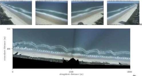
In the present work three sandbar datasets from different sources were used. One set consists of in-situ profile mea-surements, and the other two were obtained using Argus imaging stations (Holman and Stanley, 2007). An Argus station consists of one or more cameras pointed obliquely along the beach, providing an uninterrupted view of the nearshore zone. Each daylight hour, all cameras acquire a time-exposure image (e.g. Fig. 2a) created by averaging over 1200 consecutive images collected at 2 Hz. This averages the individual breaking waves to reveal one or more smooth white bands of breaking waves. The oblique images of the in-dividual cameras can be merged and rectified (Holland et al., 1997) to yield a single planview image (e.g. Fig. 2b). The continuous high-intensity bands that are manifested in the planview images serve as a reasonable estimate for the sub-merged sandbars (Lippmann and Holman, 1989), and can be extracted from the images by the alongshore tracking of intensity maxima (van Enckevort and Ruessink, 2001) (e.g. Fig. 2b). Since sandbar migration over a single hour is insignificant relative to the accuracy of the rectification and extraction processes, barline extraction is usually performed on a single image at the lowest tide of each day, when the breaking patterns are most pronounced.
The first dataset was gathered by the Argus station at Surfers Paradise, northern Gold Coast, Queensland, Aus-tralia (Turner et al., 2004), in the period between 15 July 1999 and 10 April 2007. The second dataset was acquired from the Argus station situated near Egmond, the Netherlands. This dataset starts at 31 May 1999 and con-tinues to 26 April 2007, but data from the years 2000 and 2005 are almost entirely missing due to technical problems.
Barlines were extracted over a stretch of coast of 3 km for the Gold Coast images and 4 km for the Egmond images. Oc-casionally, sandbar positions could not be computed due to poor image quality (fog or rain droplets on one of the cam-era lenses), conditions when waves were too low to break, or the malfunctioning of the video acquisition system. To create a continuous time-series dataset, gaps smaller than 2 days were filled by linear interpolation between adjacent breaking-based observations. The majority of the gaps in the data were caused by images that revealed no clear breaker pattern because they were collected during low-energy ditions. Because bar migration is very small under these con-ditions, we expect that the linear interpolation will have lit-tle effect on the results of the nonlinearity detection method. After the extraction process the barlines were averaged in the alongshore direction to yield a single cross-shore position per sandbar each day. From this dataset the periods and sandbars with the best barline accuracy and the most natural sandbar behavior were selected (e.g. the seamost positioned sandbar at Egmond was discarded because waves were seldom high enough to reveal its position; the first part of the inner sand-bar at the Gold Coast was left out of the analysis because a beach nourishment was carried out during that period; the decay phases of the outer sandbar at the Gold Coast were not taken into account because the process of extracting barlines from the images was less accurate for these periods). The resulting Gold Coast dataset containing 2143 days of outer sandbar positions and 1914 days of inner sandbar positions is shown in Fig. 3a. The Egmond dataset containing 1865 days of both inner and outer sandbar measurements is depicted in Fig. 3b.
video-observed sandbar position was projected on a fixed water level (≈0.5 m below mean sea level) using in-situ mea-surements of tidal water levels at Egmond, and the astronom-ical tide at the Gold Coast, because data on the actual tide (which can differ due to local conditions) was not available for that station.
The third dataset consists of measured water depths ob-tained from the Hazaki Oceanographical Research Station (HORS), located on the Hazaki coast of Japan facing the Pacific Ocean. At HORS, profile measurements were per-formed along a 427 m long pier, daily from 1 January 1987 to 1 August 1999, except for weekends and holidays. The profile measurements with a resolution of 5 m, can be used to infer the cross-shore sandbar position. Most of the time there was only a single sandbar, so the position of the sandbar crest was defined as the local maximum elevation of at least 0.3 m at the seamost side of each profile. Although a second, inner sandbar could sometimes be distinguished, the total amount of inner sandbar positions was too small to be considered in the analysis. The parts of the data in which variations in pro-file height were below the threshold of the local maximum for more than three consecutive days were left out of the anal-ysis. Gaps in the cross-shore sandbar positions time-series smaller than four days were filled using a LOESS interpola-tion filter (Cleveland and Devlin, 1988). The resulting time-series of 3861 sandbar positions is depicted in Fig. 3c. Note that the gray lines in Figs. 3a–c indicate bad-quality data that were left out of the analysis. Extensive reviews of the HORS dataset are given in Kuriyama (2002) and in Kuriyama and Yanagishima (2006).
Data on the predominant external inputs for driving sand-bar variability, the offshore waves, were acquired from sev-eral sources. The offshore waves can be represented by their root-mean-squared wave height Hrms, peak wave pe-riodTpeakand wave direction relative to the shore normalφ. For the Gold Coast dataset, the variablesHrmsandTpeakwere obtained each thirty minutes from the Gold Coast waverider buoy, located about 2 km offshore of the study area, in 16 m water depth. Directional informationφwas collected hourly by the Brisbane waverider buoy located some 10 km offshore in 70 m water depth, about 100 km north of the study area. The wave climate at Egmond was measured hourly by the IJmuiden06 waverider buoy, located some 40 km offshore in 21 m water depth. At HORS, data on the day-averaged wave heights and periods were available from an ultrasonic wave gage located 5 km offshore in 24 m water depth. Because no directional information was available, the predominant direc-tion of incoming waves at HORS (30◦) was used when nec-essary.
The three variables expressing the properties of the incom-ing waves were combined into the wave height at breakincom-ing (Plant et al., 1999)
Hb=
γ
g 15
Hrms2 ·cg·cos(φ)
25
, (6)
where the offshore group velocity cg was computed using linear wave theory involving Tpeak and the water depth at the location of the offshore wave measurement, the gravi-tational accelerationgis 9.81 m s−2, and the wave height to water depth ratio at breakingγ was set to 0.4, a typical field value (Thornton and Guza, 1983). If multiple observations of Hrms, Tpeak andφ were available during a day, Hb was computed from each 3-tuple and then averaged to yield a sin-gle value between two subsequent sandbar observations. The time-averagedHbvalue was given the time index of the sec-ond observation, which explains the formulation in Eq. (1). MissingHbvalues were filled by linear interpolation. The time-series of the hydrodynamic data are depicted in Fig. 3d– f.
As noted in Sect. 2, the incoming waves have to be consid-ered as an external forcing factor because they are measured offshore. Moreover, the actual wave forcing at different lo-cations in the cross-shore direction might be only weakly re-lated to the offshore-measured forcing. For the outer sandbar this is not very problematic, because the properties of the waves do not change much between the offshore location of the buoy and the location of the outer sandbar. Waves that break on the inner sandbar however, have undergone a com-plex transformation before their arrival. If the waves are high enough, they break on the outer sandbar first. The waves then reform in the trough between the outer and the inner sandbar, and break again on the inner sandbar. Although no surfzone wave measurements are available, it is still possible to obtain information on changing wave properties in the nearshore by using a wave-transformation model. Such models compute the various changing properties of the waves over a cross-shore profile, based on offcross-shore-measured wave properties. Whereas computing surfzone wave properties for the HORS profile dataset would not make much sense because there is only a single sandbar, very few profile data for the locations in the Argus datasets were available. For the Gold Coast a single profile measurement was performed in June, 2002 and at Egmond five profiles measured annually in 1999–2003 were available.
the Battjes-Janssen model, based on a only a few measured profiles, is by no means an accurate representation of the ac-tual wave heights. However, given the available models and information this is the only way to infer at least some prop-erties of the waves at different positions in the profile. This information can then be used to investigate the importance of the external forcing and where it is measured.
As can be inferred from Fig. 3 the most pronounced fea-ture of sandbar behavior is the rapid offshore movement un-der high wave energy conditions (storms), and the relatively slow onshore return under relatively quiescent wave condi-tions. There is however a large difference between the sites in the sensitivity of sandbar migration to the height of the wave forcing. The sandbars at the Gold Coast, showing a maximum migration of 75 m d−1, are the most responsive to high energy conditions. Whereas the wave height at breaking at HORS can be much larger during the depressions in winter and the typhoons in autumn, the maximum observed sandbar migration at HORS is 50 m d−1. At Egmond the sandbars are even less-responsive to high energy conditions, showing a maximum of 30 m d−1. Patterns of alternating directions of sandbar migration are linked to the external forcing and might reflect the seasonal weather patterns as well. How-ever, the resulting net migration of each sandbar crest posi-tion is always offshore. When a sandbar continues to move offshore, the water depth above the sandbar increases (due to the beach slope) until finally the depth becomes too large for incoming waves to break. At that point the driving force that maintains the sandbar ceases, and the sandbar disintegrates. In the first part of the HORS dataset in Fig. 3c this happens almost every year near the end of the typhoon season, after which a new sandbar is formed close to the shore. This 1-year period cyclic behavior changes after 1993, probably due to changing wave conditions (Kuriyama and Yanagishima, 2006). At the Gold Coast the outer sandbar also decays after one or more major storms (e.g. early 2006 in Fig. 3a). After such an event the existing inner sandbar moves seaward and becomes the new outer sandbar, while a new inner sandbar is formed at the shore. In the period shown in Fig. 3a the to-tal lifespan of a sandbar, from its formation at the shoreline to its decay seaward of the breaker zone, is≈4 years, giving rise to a periodicity with an interval of≈2 years. Although at Egmond no sandbar decay event takes place during the stud-ied period, it is known from earlier studies of the Dutch coast that the same pattern of formation and disintegration of sand-bars is also present at Egmond, be it at a much slower pace of≈15 years (Wijnberg and Terwindt, 1995).
As mentioned before, at Egmond there is a third sandbar at the seamost edge of the breaker zone which could not ac-curately be analyzed from the images. Although here we call the second sandbar counted from the shore the outer sandbar, it is occasionally sheltered from very high waves by the actual outer sandbar, as becomes clear from a com-parison between Fig. 3e and h. This means that the sec-ond sandbar at Egmsec-ond may show behavior that is more
intermediate between inner and outer sandbars. Together, all these different sandbars at locations with various boundary conditions are a good representation of the entire spectrum of sandbar behavior and comprise a broad basis for general-izing the results of the nonlinearity analysis.
3.2 Setup
To investigate the nonlinearity related to cross-shore sandbar positions and wave forcing, the MDVS method was applied to the Gold Coast, Egmond and HORS datasets. The system state variable was the cross-shore sandbar position, andHb andHrmscomputed at different locations were used as forc-ing variables. Inner and outer sandbars were studied in sep-arate experiments. The effect of using offshore and locally computed forcings was also studied by usingHrmscomputed at the outer sandbar as forcing for the outer sandbar, andHrms computed in the trough between the outer and inner sandbars as forcing for the inner sandbar. For comparison, Hb was also used as forcing variable in additional experiments.
First, the variables were embedded in state space. Al-though several methods exist to find optimal values for the lag time and embedding dimension of univariate data (e.g. first zero of autocorrelation, mutual information), find-ing these values for interdependent multivariate data is not straightforward. The dataset consists of one low-tide image or one profile measurement per day, so a lag time shorter than 1 day could not easily be achieved. A lag time that is too small relative to the timescale of the studied char-acteristics becomes only a problem when the embedding dimension is very small too (Kantz and Schreiber, 1997). Since several embedding dimensions were tested here, no detailed investigation into the optimal lag time needs to be performed, so the lag time was set to 1 day. Embedding dimensionsm=o=1, . . . ,10 were tested in separate exper-iments. The capacity of linear models to simulate nonlinear dynamics increases for larger embedding dimensions. As a result, no noticeable performance difference between linear and nonlinear models was achieved for embedding dimen-sions larger than 6, so the presentation of the results is limited tom=o=1, . . . ,6.
For each sandbar, errors were computed as the mean out-of-sample absolute prediction error over all but the first m
(a)
alongshore distance (m)
cr
os
s-sh
or
e
d
is
ta
n
ce
(m
)
0 400 800
1500 3000
(b)
Fig. 2. Argus camera images, merged plan view and tracked barlines.
(a) Time-exposure Argus images of all cameras; the high-intensity bands in each image are due to persistent wave breaking on the sandbars. (b) Tracked outer (solid) and inner (dashed) barlines in plan view.
models becomes more pronounced with increasing predic-tion horizons (e.g. Sugihara and May, 1990). Therefore not only the one-lag (day) ahead prediction (n=1) was used, as is usual in the DVS method, but also larger prediction hori-zons up ton=14 were tested. An example of observations and actual linear and nonlinear model outputs for even longer prediction horizons is given in Pape et al. (2007). Since we are primarily interested in differences between models based on different numbers of neighbors, the error is represented as the percentage of the error of an ARX model that is based on all samples. The local models and the full ARX model to which they are compared are based on the same lag time, embedding dimension and prediction horizon, ensuring a fair comparison between the local and global models.
Results were obtained for different weight values of the system state weightwx, and the forcing weightwf. Weight ratios were taken from the set defined in Eq. (5) withq=8, resulting in a total of 17 weight ratios. Figure 4 shows the results of the MDVS method for all sandbars in the three datasets with different forcings. In each image the horizon-tal axis represents the number of neighbors that was used to build a model for each sample, and the vertical axis the weight ratio between the forcing and system state variable that was used in the nearest neighbor distance function. In this fashion, the course of the error and the location of the minimum error can easily be observed in the pictures. For most embedding dimensions the location of the optimum and
the course of the error were very similar (although the ac-tual values could differ). Therefore, the results were aver-aged overm=o=1, . . . ,6. As a result, any difference in the location of the optimum among different embedding dimen-sions becomes visible as a scattered pattern (e.g. Fig. 4f). For shorter prediction horizons the results of different embedding dimensions were reasonably close, but for prediction hori-zons larger than≈7 days, often no clear optimum or other meaningful patterns were visible. To give an indication how the results of the MDVS method change with increasing pre-diction horizons, the results for bothn=1 andn=7 are shown in Fig. 4.
3.3 Interpretation of MDVS results
for the outer sandbar at the Gold Coast (Fig. 4c). The dif-ferences are smaller for the other sandbars, ranging from 6% for the inner sandbar at the Gold Coast (Fig. 4d) to only 1.2% for the sandbar at HORS (Fig. 4i). While nonlinear models outperform linear models for all cases considered, the effects of nonlinearity are generally small.
Not only the value of the optimum error percentage varies among different sandbars, also the location of the optimum relative to the weight ratios differs in the images in Fig. 4. In most images the error decreases when the weight of the forcing variablewf increases (from bottom to top), but starts to decrease again when this weight increases beyond a cer-tain value. It can be deduced from a comparison with Fig. 1d that this is caused by nonlinearity that is related to both the forcing and system state variable. For some results how-ever (e.g. Fig. 4a, d and c), the error does not start to in-crease again when the wf : wx ratio becomes large. In these cases the optimum performance is achieved forwx=0, which means that similarities in the system state are totally discarded in the process of neighbor selection. This situa-tion is the same as the outcome of Fig. 1b, in which only the forcing factor acts nonlinearly on the system. Unlike Fig. 1b, the course of the error in the images in Fig. 4 some-times also reaches an optimum for a certainkwhenwf=0 (e.g. Fig. 4d), but that does not necessarily mean that the re-lation between subsequent system states is nonlinear. The reason this is not taken as an indication for nonlinearity in the system state variable, is that the dependency between the system state and the forcing works in both ways. Although this cannot be true in a strict sense, this can be explained by a further analysis of the lag time in relation to the nature of sandbar behavior. During the onset of a storm, a sand-bar moves offshore rapidly and stays there during the rest of the storm. When after the storm the energy of the waves becomes smaller, the sandbar starts to move onshore. Since most storms last for several days, seaward located sandbar positions often coincide with high-energy conditions. When neighbors are chosen for a seaward located sandbar based on sandbar location only, the nearest neighbor algorithm will unintendedly also select high-energy conditions. In other words, the duration of the important events is large compared to the resolution of the data. However, it is still possible to in-fer something about the importance of each variable to non-linearity because the results for several embedding dimen-sions are given. Although the error might show an optimum value over the transectwf=0, the location of the optimum with respect to the weight ratiowf :wxindicates the nonlin-earity related to that variable. Only when both variables act nonlinearly on the system the error will reach its minimum when both weights have nonzero values. For some of the re-sults (e.g. Fig. 4g, i) this is clearly the case, while for other results the optimum is reached whenwx=0 (e.g. Fig. 4a, c).
Figure 4 also shows the results for different forcing variables:Hb;Hrms computed at the outer sandbar, which was used as forcing for the outer sandbar; and Hrms
computed in the trough between the outer and inner sandbar, used as forcing for the inner sandbar. WhenHrmswas used for the outer sandbar instead ofHb, the location of the opti-mum with respect to the number of neighbors or the weight ratios did not change much (see Fig. 4a, c, e, g). This was as expected, because the wave height at breakingHbandHrms computed at the outer sandbar are very well correlated (see Fig. 3). The most noticeable difference between usingHb andHrmsas forcings for the inner sandbars (Fig. 4b, d, f, h) is the shift of the minimum error with respect to the weight ratio on the vertical axes. WhenHbis used as forcing, the optimum is reached when bothwf andwxhave nonzero val-ues, indicating nonlinearity associated with both variables. Models that useHrms as forcing factor reach their optimum performance when wx=0, so selecting neighbors based on similarity in locally computed forcings only, gave optimal re-sults. In other words, also considering similar system states in the process of model building did not result in a reduction of the prediction error. This indicates that given the locally computed forcing, a linear relation between subsequent sand-bar positions suffices.
When nonlinearity is present, the performance difference between linear and nonlinear models will become more pronounced with increasing prediction horizon. For most MDVS results this was indeed the case up to at leastn=10. Surprisingly, this trend was not found in the results of the outer sandbar at Egmond (Fig. 4e and g), up to at leastn=14. This can partially be attributed to the fact that the minima of different embedding dimensions become spread out for in-creasingn, and do not overlap. In other results with scattered minimum error values (e.g. Fig. 4f and i) the performance difference also started to diminish for n>10. Using iter-ative prediction based on previous model outcomes allows the nonlinear models to wander further away from the ob-served system state. For linear models this happens more slowly. Given the small differences between linear and non-linear models, and the scattered locations and values of the minimum errors among the different embedding dimensions, this is another possible cause for the decreasing difference between both types of models for largen.
3.4 Discussion of the MDVS results
time (year)
p
os
it
io
n
(m
)
250 500 750
2000 2002 2004 2006
(a) time (year)
p
os
it
io
n
(m
)
250 500 750
2000 2002 2004 2006
(b) time (year)
p
os
it
io
n
(m
)
250 500 750
1988 1990 1992 1994 1996 1998
(c)
time (year)
Hb
(m
)
0 2 4
2000 2002 2004 2006
(d) time (year)
Hb
(m
)
0 2 4
2000 2002 2004 2006
(e) time (year)
Hb
(m
)
0 2 4
1988 1990 1992 1994 1996 1998
(f)
time (year)
H
r
m
s
(m
)
at outer bar at trough
0 2 4
2000 2002 2004 2006
(g) time (year)
H
r
m
s
(m
)
at outer bar at trough
0 2 4
2000 2002 2004 2006
(h) time (year)
H
r
m
s
(m
)
offshore
0 2 4
1988 1990 1992 1994 1996 1998
(i)
Fig. 3. Overview of the variables in the datasets: (a) sandbar positions at the Gold Coast; (b) sandbar positions at Egmond; (c) sandbar positions at HORS; (d) hydrodynamic data at the Gold Coast; (e) hydrodynamic data at Egmond; (f) hydrodynamic data at HORS; (g)Hrms
over profile at the Gold Coast; (h)Hrmsover profile at Egmond; (i) offshoreHrmsat HORS.
causes a change in both the location of the highest break-ing intensity relative to the sandbar crest, and possibly also in the actual sandbar position. The linear part of the migra-tion induced by the change of the highest breaker intensity can be represented by linear models for embedding dimen-sions larger than one. Still, it might be that the nonlinear part of this relation affects the results of the MDVS outcome.
Another step in the data accumulation procedure involv-ing Argus images, is the averaginvolv-ing process that is applied to find the mean cross-shore sandbar position. As can be seen in Fig. 2, the cross-shore position can vary in the alongshore direction. If the migration of a sandbar depends nonlinearly on its cross-shore position, the different alongshore parts of the sandbar might migrate different distances or even in dif-ferent directions under the same forcing conditions. Some of this potential nonlinearity is averaged out by taking the mean cross-shore sandbar position. On the other hand, two sandbars with the same mean cross-shore position but differ-ent alongshore variability might react differdiffer-ent to the same forcing conditions. Part of the nonlinearity found in the observed mean cross-shore position might thus be due to discarding alongshore variability in the models. For exam-ple, the outer bar at the Gold Coast often contains a lot of alongshore variability (e.g. Fig. 2), while the difference be-tween linear and nonlinear models also is the largest. How-ever, site-specific issues during data-collection might have introduced additional noise, thus obscuring the differences between sites. At the Gold Coast, breaker patterns are well-pronounced, light and atmospheric conditions are excellent,
and the cameras are steady and almost never malfunction. The images in the Egmond dataset are much more difficult to interpret due to less perfect conditions, especially the vi-bration of the 50 m high tower in the wind. Sandbar crest po-sitions in the HORS dataset are defined as the most seaward located optimum in the profile, which might not always be well-pronounced. For the outer sandbar at the Gold Coast the effects of nonlinearity are most pronounced, but it might well be that at other sites the effects of nonlinearity are reduced by larger amounts of noise introduced during data gathering.
k k w ei gh t ra ti o ( wf : wx ) 0:1 2:1 1:1 1:2 1:0 500
500 1000 1500 1000 1500
n= 1 n= 7
≥100 92.5 85 er ro r %
(a) k k
w ei gh t ra ti o ( wf : wx ) 0:1 2:1 1:1 1:2 1:0 500
500 1000 1500 1000 1500
n= 1 n= 7
≥100 97 94 er ro r % (b) k k w ei gh t ra ti o ( wf : wx ) 0:1 2:1 1:1 1:2 1:0 500
500 1000 1500 1000 1500
n= 1 n= 7
≥100 92.5 85 er ro r %
(c) k k
w ei gh t ra ti o ( wf : wx ) 0:1 2:1 1:1 1:2 1:0 500
500 1000 1500 1000 1500
n= 1 n= 7
≥100 97 94 er ro r % (d) k k w ei gh t ra ti o ( wf : wx ) 0:1 2:1 1:1 1:2 1:0 500
500 1000 1500 1000 1500
n= 1 n= 7
≥100 98.5 97 er ro r %
(e) k k
w ei gh t ra ti o ( wf : wx ) 0:1 2:1 1:1 1:2 1:0 500
500 1000 1500 1000 1500
n= 1 n= 7
≥100 98.5 97 er ro r % (f) k k w ei gh t ra ti o ( wf : wx ) 0:1 2:1 1:1 1:2 1:0 500
500 1000 1500 1000 1500
n= 1 n= 7
≥100 98.5 97 er ro r %
(g) k k
w ei gh t ra ti o ( wf : wx ) 0:1 2:1 1:1 1:2 1:0 500
500 1000 1500 1000 1500
n= 1 n= 7
≥100 98.5 97 er ro r % (h) k k w ei gh t ra ti o ( wf : wx ) 0:1 2:1 1:1 1:2 1:0 1000
1000 2000 3000 2000 3000
n= 1 n= 7
≥100 99.4 98.8 er ro r % (i)
Fig. 4. MDVS results for all sandbars with different forcings (HbandHrms) and prediction horizonsn. Error values are computed as the
mean out-of-sample absolute error, averaged overm=o=1, . . . ,6. The images contain the error percentages relative to a full linear model, at each number of neighborsk, and weight ratiowf :wx. (a) Gold Coast, outer sandbar, forcing:Hb. (b) Gold Coast, inner sandbar, forcing:
Hb. (c) Gold Coast, outer sandbar, forcing:Hrmsat outer sandbar. (d) Gold Coast, inner sandbar, forcing:Hrmsat trough. (e) Egmond, outer
sandbar, forcing:Hb. (f) Egmond, inner sandbar, forcing: Hb. (g) Egmond, outer sandbar, forcing: Hrmsat outer sandbar. (h) Egmond,
inner sandbar, forcing:Hrmsat trough. (i) HORS, forcing:Hb.
An additional reason for the variations in the importance of nonlinearity among different sandbars might be found in the available amount of similar states. In the MDVS re-sults of all sandbars, the optimum number of neighbors is reached within the available amount of samples. However,
many similar states in terms of sandbar position can be found by the nearest neighbor algorithm. Only when models are based on several hundreds of samples, the neighborhood con-tains enough different samples for the effect of nonlinearity in the system state to become more important than noise re-duction (e.g. Fig. 4e, g). On the other hand, a comparison with the HORS dataset in Fig. 3c and its MDVS results in Fig. 4i reveals that differences in optimumkand the relation to sandbar behavior cannot immediately be inferred from the MDVS results. Apart from the differences that arise from data-gathering methods, the available amount of data relative to the length of the cyclic patterns in the sandbar’s behavior determines the location of the optimal number of neighbors. While in all datasets used here the available amount of sam-ples is only two or three times as large as the optimal number of neighbors, the true effect of availability of similar states can only be investigated in detail when the amount of cycles in sandbar behavior is close to the optimalk.
As discussed in Sect. 3.3, the MDVS results can be inter-preted in terms of the importance of nonlinearity for both the system state and the forcing variable. Sugihara (1994) dis-cusses a case with a single variable and noise, in which the variability induced by the noise process causes the system to behave in a different mode (e.g. move toward or away from a stable state) for different noise levels. Similarly, it might be possible that a sandbar system changes between different modes of behavior, which means that nonlinearities associ-ated with the forcing and the dynamics of the sandbar sys-tem are inherently inseparable. If the sandbar syssys-tem were to change between different modes of behavior, the total be-havior of the system would still be nonlinear. Whereas the MDVS results only show nonlinearity for the entire system, that is over all values of the variables, investigating the im-portance of nonlinearity for different values of each variable might reveal these different modes. To examine the possi-bility of different modes of behavior, the performance dif-ference between linear and nonlinear models was evaluated at individual values of the cross-shore sandbar position and wave forcing variables. This analysis included all sandbar cases and prediction horizons up ton=14, but no relation was found whatsoever. We have to admit that the significance of any relation would have been doubtful given the amount of data and the noise in the available data.
3.5 Implications for modeling
Our findings that linear models can predict observed cross-shore sandbar behavior almost as accurate as nonlinear mod-els implies that simple data-driven modmod-els might suffice to model observed cross-shore bar behavior. This is consistent with Pape et al. (2007), who also found small differences be-tween the performance of several linear and nonlinear data-driven models, even over prediction horizons up to 2 year. Also Plant et al. (1999) found that a relatively simple model (calibrated on the observations) could explain up to 80% of
the observed bar position variability. There are two possible causes for the small difference between linear and nonlinear models: the system is actually linear, or the data gathered from the system is dominated by noise.
If cross-shore sandbar behavior is actually linear, there are important implications for the way in which morpho-logical behavior can best be predicted. Process-based mod-els that are used to describe the evolution of the nearshore zone are based on scales that are both temporally and spa-tially very small compared to a sandbar and its behavior. Whereas process-based models can compute the evolution of the morphology for the entire nearshore zone, the data-driven models used in the present work are based on a small number of larger-scale variables that represent the significant changes in underlying morphology (Plant et al., 2001). The interpre-tation that sandbar behavior is linear might be founded in the fact that small-scale physical processes can together evolve towards a simple attractor state. While process-based mod-els based on sediment flux computations in fine grids and small timesteps might suffer from numerical instability, or the build-up of errors in the process formulations, statistical models might perform better on larger prediction horizons because they are based on stable statistical properties of at-tractor states. The long-term evolution of the nearshore zone might therefore be predicted more accurately using relatively simple models based on just a few large-scale variables. For a more elaborate discussion, see Southgate and M¨oller (2000) and Werner (1999, 2003).
On the other hand, if the small difference between linear and nonlinear models is caused by the presence of noise, the underlying system might still be highly nonlinear. As long as the noise is not reduced, there is no way to rule out the possibility that the underlying system is actually highly non-linear, meaning that a nonlinear model might be much better in predicting the actual system state. More complex non-linear models such as the process-based models discussed before might thus be able to model the actual morphology and sandbar position more accurately. There is however no way to validate this claim. Since the datasets used in the present work are among the highest quality and resolu-tion datasets in existence, the accuracy of any type of model would have to be validated against this kind of data. For pre-diction purposes, the question is not how accurate a model can predict actual sandbar positions, but how accurate it predicts the observed data. In case of the Argus data this would not necessarily mean the prediction of the sandbar crest position, but could also be the position of the maxi-mum roller dissipation, the analog of image breaker intensity (Aarninkhof et al., 2005).
4 Conclusions
to three sandbar datasets, containing a total of five different sandbars and their corresponding external wave forcings. The results of the MDVS method revealed nonlinearity in the relations between the offshore wave forcing and sandbar migration. When wave height estimates at the location of the sandbar were used rather than offshore wave heights, the im-portance of nonlinearity related to the forcings increased rel-ative to the importance of nonlinearity related to subsequent system states. The differences between nonlinear models and a linear model were however small (the Gold Coast<15%, Egmond<6% and HORS<2%) even when sandbar positions were predicted over several days ahead. It might even be that part of the detected nonlinearity is not present in actual sand-bar behavior, but is induced by the data gathering procedure. On the other hand, the presence of noise and the relatively small amount of available data with respect to the period of the cyclic patterns in the data might obfuscate the importance of nonlinearity in the underlying system. Data similar to the sandbar datasets used in the present work are often used for calibrating and validating process-based models. Our finding that linear models are almost as accurate as nonlinear models on the sandbar datasets implies that the prediction of large-scale features in the nearshore zone might not benefit much from the use of such complex nonlinear models.
Acknowledgements. This work was supported by the Netherlands
Organization for Scientific Research (NWO) under contract 864.04.007. The Gold Coast wave and water level data were kindly made available by D. Anderson (University of New South Wales) and the Environmental Protection Agency in Queensland. The Gold Coast City Council is acknowledged for ongoing funding support to I. Turner that enables the continued operation of the Argus video station at the northern Gold Coast. We thank Y. Kuriyama for generously supplying the HORS data. The staff members at HORS are acknowledged for conducting profile measurements even during most violent typhoons.
Edited by: H. A. Dijkstra
Reviewed by: K. Bryan and another anonymous referee
References
Aarninkhof, S., Ruessink, B. G., and Roelvink, J. A.: Nearshore subtidal bathymetry from time-exposure video images, J. Geo-phys. Res., 110, C06011, doi:10.1029/2004JC002791, 2005. Abraham, F. D.: Nonlinear coherence in multivariate research:
in-variants and the reconstruction of attractors, Nonlinear Dynam-ics, Psychology and Life Sciences, 1, 7–33, 1997.
Battjes, J. A. and Janssen, J. P. F. M.: Energy loss and set-up due to breaking of random waves, in: Proceedings of the 16th Confer-ence on Coastal Engineering, 569–587, ASCE, 1978.
Battjes, J. A. and Stive, M. J. F.: Calibration and verification of a dissipation model for random breaking waves, J. Geophys. Res., 90, 9159–9167, 1985.
Box, G. E. P. and Jenkins, G. M.: Time series analysis: Forecasting and control, Holden-Day, San Francisco, 1970.
Cao, L., Mees, A., and Judd, K.: Dynamics from multivariate time series, Physica D, 121, 75–88, 1998.
Casdagli, M.: A dynamical systems approach to modeling input-output systems, 265–281, Addison-Wesley, 1992.
Casdagli, M. C. and Weigend, A. S.: Exploring the continuum between deterministic and stochastic modeling, in: Time Se-ries Prediction: Forecasting the Future and Understanding the Past, edited by Weigend, A. S. and Gershenfeld, N. A., 347–366, Addison-Wesley, Massachusetts, 1993.
Cleveland, W. S. and Devlin, S. J.: Locally weighted regression: an approach to regression analysis by local fitting, J. Am. Stat. Assoc., 83, 596–610, 1988.
Elgar, S.: Coastal profile at Duck, North Carolina: A cautionary note, J. Geophys. Res., 106, 4625–4627, 2001.
Gallagher, E. L., Elgar, S., and Guza, R. T.: Observations of sand bar evolution on a natural beach, J. Geophys. Res., 103, 3203– 3215, 1998.
Garcia, S. P. and Almeida, J. S.: Multivariate phase space reconstruction by nearest neighbor embedding with different time delays, Phys. Rev. E, 72, 027205, doi: 10.1103/Phys-RevE.72.027205, 2005.
Hoefel, F. and Elgar, S.: Wave-induced sediment transport and sandbar migration, Science, 299, 1885–1887, 2003.
Holland, K. T., Holman, R. A., Lippmann, T. C., Stanley, J., and Plant, N. G.: Practical use of video imagery in nearshore oceano-graphic field studies, J. Oceanic Engineering, 22, 81–92, 1997. Holman, R. A. and Stanley, J.: The history and technical capabilities
of Argus, Coast. Eng., 54, 477–491, 2007.
Jaffe, B. E. and Rubin, D. M.: Using nonlinear forecasting to learn the magnitude and phasing of time-varying sediment suspension in the surf zone, J. Geophys. Res., 101, 14 283–14 296, 1996. Kantz, H. and Schreiber, T.: Nonlinear time series analysis,
Cam-bridge University Press, CamCam-bridge, first Edn., 1997.
Kuriyama, Y.: Medium-term bar behavior and associated sedi-ment transport at Hasaki, Japan, J. Geophys. Res., 107, 3132, doi:10.1029/2001JC000899, 2002.
Kuriyama, Y. and Yanagishima, S.: Medium-term variations of bar properties and their linkages with environmental factors at HORS, Tech. Rep. 4, Kashima port and airport research institute, Kashima, 2006.
Lippmann, T. C. and Holman, R. A.: Quantification of sand bar morphology: a video technique based on wave dissipation, J. Geophys. Res., 94, 995–1011, 1989.
Pape, L., Ruessink, B. G., Wiering, M. A., and Turner, I. L.: Re-current neural network modeling of nearshore sandbar behavior, Neural Networks, 20, 509–518, 2007.
Plant, N. G., Holman, R. A., Freilich, M. H., and Birkemeier, W. A.: A simple model for interannual sandbar behavior, J. Geophys. Res., 104, 15 755–15 776, 1999.
Plant, N. G., Freilich, M. H., and Holman, R. A.: Role of morpho-logic feedback in surf zone sandbar response, J. Geophys. Res., 106, 973–989, 2001.
Plant, N. G., Holland, T., and Holman, R. A.: A dynamical attrac-tor governs beach response to sattrac-torms, Geophys. Res. Lett., 33, L17607, doi:10.1029/2006GL027105, 2006.
Reniers, A. J. H. M. and Battjes, J. A.: A laboratory study of long-shore currents over barred and non-barred beaches, Coast. Eng., 30, 1–21, 1997.
Eng., 21, 163–191, 1993.
Rubin, D. M.: Forecasting techniques, underlying physics and ap-plications, chap. 5, SEPM Short Course No. 36, Society for Sed-imentary Geology, 1995.
Ruessink, B. G., Kuriyama, Y., Reniers, A. J. H. M., Roelvink, J. A., and Walstra, D. J. R.: Modeling cross-shore sandbar be-havior on the timescale of weeks, J. Geophys. Res., 112, F03010, doi:10.1029/2006JF000730, 2007.
Sauer, T., Yorke, J. A., and Casdagli, M.: Embedology, J. Stat. Phys., 65, 579–616, 1991.
Schreiber, T. and Schmitz, A.: Surrogate time series, Physica D, 142, 346–382, 2000.
Southgate, H. N. and M¨oller, I.: Fractal properties of beach pro-file evolution at Duck, North Carolina, J. Geophys. Res., 105, 11 489–11 507, 2000.
Sugihara, G.: Nonlinear Forecasting for the Classification of Nat-ural Time Series, Philosophical Transactions: Physical Sciences and Engineering, 348, 477–495, 1994.
Sugihara, G. and May, R. M.: Nonlinear forecasting as a way of dis-tinguishing chaos from measurement error in time series, Nature, 344, 734–742, 1990.
Takens, F.: Detecting strange attractors in turbulence, in: Dynami-cal systems and turbulence, Lecture notes in mathematics, 898, 366–381, Springer, Berlin, 1981.
Thornton, E. B. and Guza, R. T.: Transformation of wave height distribution, J. Geophys. Res., 88, 5925–5938, 1983.
Turner, I. L., Aarninkhof, S. G. J., Dronkers, T. D. T., and McGrath, J.: CZM applications of Argus coastal imaging at the Gold Coast, Australia, J. Coastal Res., 20, 739–752, 2004.
van Enckevort, I. M. J. and Ruessink, B. G.: Effects of hydrody-namics and bathymetry on video estimates of nearshore sandbar position, J. Geophys. Res., 106, 16 969–16 979, 2001.
van Rijn, L. C., Walstra, D. J. R., Grasmeijer, B., Sutherland, J., Pan, S., and Sierra, J. P.: The predictability of cross-shore bed evolution of sandy beaches at the time scale of storms and sea-sons using process-based profile models, Coast. Eng., 47, 295-327, 2003.
Werner, B. T.: Complexity in natural landform patterns, Science, 284, 102–104, 1999.
Werner, B. T.: Modeling landforms as self-organized, hierarchi-cal dynamihierarchi-cal systems, Geophysihierarchi-cal Monograph, 135, 133–150, AGU Press, 2003.