Testing and modelling autoregressive conditional heteroskedasticity of streamﬂow processes

(1)

Nonlinear Processes in Geophysics (2005) 12: 55–66 SRef-ID: 1607-7946/npg/2005-12-55

European Geosciences Union

Nonlinear Processes

in Geophysics

Testing and modelling autoregressive

conditional heteroskedasticity of streamflow processes

W. Wang1, 2, P. H. A. J. M. Van Gelder2, J. K. Vrijling2, and J. Ma3

1_{Faculty of Water Resources and Environment, Hohai University, Nanjing, 210098, China}

2_{Faculty of Civil Engineering & Geosciences, Section of Hydraulic Engineering, Delft University of Technology, P.O.Box} 5048, 2600 GA Delft, The Netherlands

3_{Yellow River Conservancy Commission, Hydrology Bureau, Zhengzhou, 450004, China}

Received: 24 May 2004 – Revised: 15 December 2004 – Accepted: 5 January 2005 – Published: 21 January 2005 Part of Special Issue “Nonlinear deterministic dynamics in hydrologic systems: present activities and future challenges”

Abstract. Conventional streamflow models operate under the assumption of constant variance or season-dependent variances (e.g. ARMA (AutoRegressive Moving Average) models for deseasonalized streamflow series and PARMA (Periodic AutoRegressive Moving Average) models for sea-sonal streamflow series). However, with McLeod-Li test and Engle’s Lagrange Multiplier test, clear evidences are found for the existence of autoregressive conditional het-eroskedasticity (i.e. the ARCH (AutoRegressive Conditional Heteroskedasticity) effect), a nonlinear phenomenon of the variance behaviour, in the residual series from linear models fitted to daily and monthly streamflow processes of the up-per Yellow River, China. It is shown that the major cause of the ARCH effect is the seasonal variation in variance of the residual series. However, while the seasonal variation in variance can fully explain the ARCH effect for monthly streamflow, it is only a partial explanation for daily flow. It is also shown that while the periodic autoregressive mov-ing average model is adequate in modellmov-ing monthly flows, no model is adequate in modelling daily streamflow pro-cesses because none of the conventional time series mod-els takes the seasonal variation in variance, as well as the ARCH effect in the residuals, into account. Therefore, an ARMA-GARCH (Generalized AutoRegressive Conditional Heteroskedasticity) error model is proposed to capture the ARCH effect present in daily streamflow series, as well as to preserve seasonal variation in variance in the residuals. The ARMA-GARCH error model combines an ARMA model for modelling the mean behaviour and a GARCH model for modelling the variance behaviour of the residuals from the ARMA model. Since the GARCH model is not followed widely in statistical hydrology, the work can be a useful

ad-Correspondence to: W. Wang

([email protected])

dition in terms of statistical modelling of daily streamflow processes for the hydrological community.

1 Introduction to autoregressive conditional het-eroskedasticity

When modelling hydrologic time series, we usually focus on modelling and predicting the mean behaviour, or the first order moments, and are rarely concerned with the condi-tional variance, or their second order moments, although unconditional season-dependent variances are usually con-sidered. The increased importance played by risk and un-certainty considerations in water resources management and flood control practice, as well as in modern hydrology the-ory, however, has necessitated the development of new time series techniques that allow for the modelling of time varying variances.

ARCH-type models, which originate from econometrics, give us an appropriate framework for studying this prob-lem. Volatility (i.e. time-varying variance) clustering, in which large changes tend to follow large changes, and small changes tend to follow small changes, has been well recognized in financial time series. This phenomenon is called conditional heteroskedasticity, and can be modeled by ARCH-type models, including the ARCH model proposed by Engle (1982) and the later extension GARCH (general-ized ARCH) model proposed by Bollerslev (1986), etc. Ac-cordingly, when a time series exhibits autoregressive condi-tionally heteroskedasticity, we say it has the ARCH effect or GARCH effect. ARCH-type models have been widely used to model the ARCH effect for economic and financial time series.

(2)

ARCH-56 W. Wang et al.: Testing and modelling autoregressive conditional heteroskedasticity

18

0 5000 10000 15000

0

1000

2000

3000

4000

5000

Day

Disc

harg

e

(cm

s)

Figure 1 Daily streamflow (m

3

/s) of the upper Yellow River at Tangnaihai

0 200 400 600 800 1000 1200 1400 1600

1-Jan 2-Mar 1-May 30-Jun 29-Aug 28-Oct 27-Dec

Date

D

ischarge (m

3 /S) daily mean_{standard deviation}

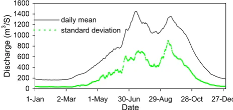
Figure 2 Variation in daily mean and standard deviation of the streamflow at Tangnaihai

0 20 40 60 80 100 Lag

0

.00

.2

0

.40

.6

0

.81

.0

AC

F

0 20 40 60 80 100 Lag

-0

.2

-0

.0

0

.2

0

.4

0

.6

0

.8

1

.0

Par

tia

l ACF

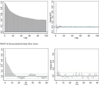
Figure 3 ACF and PACF of deseasonalized daily flow series

Fig. 1. Daily streamflow (m3/s) of the upper Yellow River at Tang-naihai.

type models can generate accurate forecasts of future volatil-ity, especially over short horizons, therefore providing a bet-ter estimate of the forecast uncertainty which is valuable for water resource management and flood control. And they take into account excess kurtosis (i.e. fat tail behaviour), which is common in hydrologic processes. Therefore, ARCH-type models could be very useful for hydrologic time se-ries modelling. Some authors propose new models to repro-duce the asymmetric periodic behaviour with large fluctua-tions around large streamflow and small fluctuafluctua-tions around small streamflow (e.g. Livina et al., 2003), which basically can be handled with those conventional time series mod-els that have taken season-dependent variance into account, such as PARMA models and deseasonalized ARMA models. However, little attention has been paid so far by the hydro-logic community to test and model the possible presence of the ARCH effect with which large fluctuations tend to follow large fluctuations, and small fluctuations tend to follow small fluctuations in streamflow series.

In this paper, we will take the daily and monthly stream-flow of the upper Yellow River at Tangnaihai in China as case study hydrologic time series to test for the existence of the ARCH effect, and propose an ARMA-GARCH error model for daily flow series. The paper is organized as fol-lows. First, the method of testing conditional heteroskedas-ticity of streamflow process is described. Then, the causes of the ARCH effect and the inadequacy of commonly used sea-sonal time series models for modelling streamflow are dis-cussed. Finally, an ARMA-GARCH error model is proposed for capturing the ARCH effect existing in daily streamflow series.

2 Case study area and data set

The case study area is the headwaters of the Yellow River, located in the northeastern Tibet Plateau. In this area, the discharge gauging station Tangnaihai has a 133 650 km2

con-18

0 5000 10000 15000

0

1000

2000

3000

4000

5000

Day

Disc

harg

e

(cm

s)

Figure 1 Daily streamflow (m

3

0 200 400 600 800 1000 1200 1400 1600

Date

D

ischarge (m

3 /S) daily mean standard deviation

0 20 40 60 80 100 Lag

0

.00

.2

0

.40

.6

0

.81

.0

AC

F

0 20 40 60 80 100 Lag

-0

.2

-0

.0

0

.2

0

.4

0

.6

0

.8

1

.0

Par

tia

l ACF

Figure 3 ACF and PACF of deseasonalized daily flow series

Fig. 2. Variation in daily mean and standard deviation of the

stream-flow at Tangnaihai.

tributing watershed, including a permanently snow-covered area of 192 km2. The length of the main channel of this wa-tershed is over 1500 km. Most of the area is 3000∼6000 meters above sea level. Snowmelt water composes about 5% of total runoff. Most rain falls in summer. Because the water-shed is partly permanently snow-covered and sparsely pop-ulated, without any large-scale hydraulic works, it is fairly pristine. The average annual runoff volume (during 1956– 2000) at Tangnaihai gauging station is 20.4 billion cubic me-ters, about 35% of the whole Yellow River Basin, and it is the major runoff producing area of the Yellow River basin. Daily average streamflow at Tangnaihai has been recorded since 1 January 1956. Monthly series is obtained from daily data by taking the average of daily discharges in every month. In this study, data from 1 January 1956 to 31 December 2000 are used. The daily streamflow series from 1956 to 2000 is plot-ted in Fig. 1, and variations in the daily mean discharge and daily standard deviation of the streamflow at Tangnaihai are shown in Fig. 2.

3 Tests for the ARCH effect of streamflow process The detection of the ARCH effect in a streamflow series is actually a test of serial independence applied to the serially uncorrelated fitting error of some model, usually a linear au-toregressive (AR) model. We assume that linear serial depen-dence inside the original series is removed with a well-fitted, pre-whitening model; any remaining serial dependence must be due to some nonlinear generating mechanism which is not captured by the model. Here, the nonlinear mechanism we are concerned with is the conditional heteroskedastic-ity. We will show that the nonlinear mechanism remaining in the pre-whitened streamflow series, namely the residual series, can be well interpreted as autoregressive conditional heteroskedasticity.

(3)

mod-W. Wang et al.: Testing and modelling autoregressive conditional heteroskedasticity 57

18

0 5000 10000 15000

0

1000

2000

3000

4000

5000

Day

Disc

harg

e

(cm

s)

Figure 1 Daily streamflow (m

3

0 200 400 600 800 1000 1200 1400 1600

Date

D

ischarge (m

3 /S) daily mean

standard deviation

0 20 40 60 80 100 Lag

0

.00

.2

0

.40

.6

0

.81

.0

AC

F

0 20 40 60 80 100 Lag

-0

.2

-0

.0

0

.2

0

.4

0

.6

0

.8

1

.0

Par

tia

l ACF

Figure 3 ACF and PACF of deseasonalized daily flow series

Fig. 3. ACF and PACF of deseasonalized daily flow series.

19

0 10 20 30 40 50 60 Lag

0.0

0

.2

0.4

0.6

0.8

1.0

AC

F

0 10 20 30 40 50 60 Lag

0.0

0

.2

0.4

0

.6

P

ar

tia

l A

C

F

Figure 4 ACF and PACF of deseasonalized monthly flow series

0 200 400 600 800 1000

Day

-1

.0

-0

.5

0

.0

0

.5

1

.0

Resi

dual

s

0 20 40 60 80 100 120

Month

-1

.5

-1

.0

-0

.5

0

.0

0.

5

1

.0

1

.5

Resi

dual

s

Figure 5 Segments of the residual series from (a) ARMA(20,1) for daily flow and (b) AR(4)

for monthly flow at Tangnaihai.

0 100 200 300 Lag

0.

00

0.

05

0.10

AC

F

0 2 4 6 8 10 12

Lag

0.

0

.1

0.2

AC

F

Figure 6 ACFs of residuals from (a) ARMA(20,1) model for daily flow and (b) AR(4) model

for monthly flow at Tangnaihai

(a)

(b)

(a)

(b)

Fig. 4. ACF and PACF of deseasonalized monthly flow series.

els; 2) deseasonalized ARMA models; and 3) periodic ARMA models. The deseasonalized modelling approach is adopted in this study. The procedure of fitting deseasonalized ARMA models to daily and monthly streamflow at Tang-naihai includes two steps. First, logarithmize both flow se-ries, and deseasonalize them by subtracting the seasonal (e.g. daily or monthly) mean values and dividing by the seasonal standard deviations of the logarithmized series. To alleviate the stochastic fluctuations of the daily means and standard deviations, we smooth them with first 8 Fourier harmonics before using them for standardization. Then, according to the ACF (AutoCorrelation Function) and PACF (Periodic Auto-Correlation Function) structures of the two series, as well as the model selection criterion AIC, two linear ARMA-type models (one ARMA(20,1) and one AR(4)) are fitted to the logarithmized and deseasonalized daily and monthly flow se-ries, respectively, following the model construction proce-dures suggested by Box and Jenkins (1976). Figures 3 and 4 show the ACF and PACF of the deseasonalized daily and monthly series. Figure 5 shows parts of the two residual se-ries obtained from the two models.

Before applying ARCH tests to the residual series, to en-sure that the null hypothesis of no ARCH effect is not re-jected due to the failure of the pre-whitening linear models, we must check the goodness-of-fit of the linear models.

Firstly, we inspect the ACF of the residuals. It is well-known that for random and independent series of lengthn, the lagk autocorrelation coefficient is normally distributed with a mean of zero and a variance of 1/n, and the 95% confidence limits are given by ±1.96/√n. The ACF plots in Fig. 6 show that there is no significant autocorrelation left in the residuals from both ARMA-type models for daily and monthly flow.

Then, more formally, we apply the Ljung-Box test (Ljung and Box, 1978) to the residual series, which tests whether the firstLautocorrelationsrˆ_k2(ε2)(k= 1, ...,L)from a pro-cess are collectively small in magnitude. Suppose we have the first L autocorrelations rˆk(ε) (k = 1, ..., L) from any ARMA(p, d, q)process. For a fixed sufficiently large L, the usual Ljung-BoxQ-statistic is given by

Q=N (N+2)

L X k=1

ˆ

r_k2(ε)

N−k, (1)

(4)

58 W. Wang et al.: Testing and modelling autoregressive conditional heteroskedasticity

19

0 10 20 30 40 50 60 Lag

0.0

0

.2

0.4

0.6

0.8

1.0

AC

F

0 10 20 30 40 50 60 Lag

0.0

0

.2

0.4

0

.6

P

ar

tia

l A

C

F

Figure 4 ACF and PACF of deseasonalized monthly flow series

0 200 400 600 800 1000

Day

-1

.0

-0

.5

0

.0

0

.5

1

.0

Resi

dual

s

0 20 40 60 80 100 120

Month

-1

.5

-1

.0

-0

.5

0

.0

0.

5

1

.0

1

.5

Resi

dual

s

0 100 200 300 Lag

0.

00

0.

05

0.10

AC

F

0 2 4 6 8 10 12 Lag

0.

0

.1

0.2

AC

F

for monthly flow at Tangnaihai

(a)

(b)

(a)

(b)

Fig. 5. Segments of the residual series from (a) ARMA(20,1) for daily flow and (b) AR(4) for monthly flow at Tangnaihai.

19

0 10 20 30 40 50 60 Lag

0.0

0

.2

0.4

0.6

0.8

1.0

AC

F

0 10 20 30 40 50 60 Lag

0.0

0

.2

0.4

0

.6

P

ar

tia

l A

C

F

Figure 4 ACF and PACF of deseasonalized monthly flow series

0 200 400 600 800 1000

Day

-1

.0

-0

.5

0

.0

0

.5

1

.0

Resi

dual

s

0 20 40 60 80 100 120

Month

-1

.5

-1

.0

-0

.5

0

.0

0.

5

1

.0

1

.5

Resi

dual

s

0 100 200 300 Lag

0.

00

0.

05

0.10

AC

F

0 2 4 6 8 10 12 Lag

0.

0

.1

0.2

AC

F

for monthly flow at Tangnaihai

(a)

(b)

(a)

(b)

Fig. 6. ACFs of residuals from (a) the ARMA(20,1) model for daily flow and (b) the AR(4) model for monthly flow at Tangnaihai.

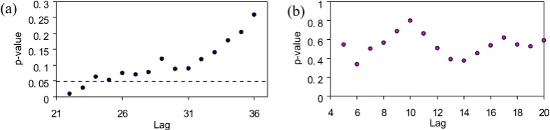
(1−α)-quantile of theχ2(L−p−q)distribution. The Ljung-Box test results for ARMA(20,1) and AR(4) are shown in Fig. 7. The p-values’ exceedance of 0.05 indicates the ac-ceptance of the null hypothesis of model adequacy at signif-icance level 0.05.

However, while the residuals seem statistically uncorre-lated according to ACF and PACF shown in Fig. 6, they are not identically distributed from visual inspection of the Fig. 5, that is, the residuals are not independent and identi-cally distributed (i.i.d.) through time. There is a tendency, especially for daily flow, that large (small) absolute values of the residual process are followed by other large (small) val-ues of unpredictable sign, which is a common behaviour of GARCH processes. Granger and Andersen (1978) found that some of the series modelled by Box and Jenkins (1976) ex-hibit autocorrelated squared residuals even though the resid-uals themselves do no seem to be correlated over time, and therefore suggested that the ACF of the squared time series could be useful in identifying nonlinear time series. Boller-slev (1986) stated that the ACF and PACF of squared process are useful in identifying and checking GARCH behaviour.

Figure 8 shows the ACFs of the squared residual series from the ARMA(20,1) model for daily flow and the AR(4) model for monthly flow at Tangnaihai. It is shown that al-though the residuals are almost uncorrelated, as shown in

Fig. 6, the squared residual series are autocorrelated, and the ACF structures of both squared residual series exhibit strong seasonality. This indicates that the variance of residual series is conditional on its past history, namely, the residual series may exhibit an ARCH effect.

There are some formal methods to test for the ARCH effect of a process, such as the McLeod-Li test (McLeod and Li, 1983), the Engle’s Lagrange Multiplier test (Engle, 1982), the BDS test (Brock et. al., 1996), etc. McLeod-Li test and Engle’s Lagrange Multiplier test are used here to check the existence of an ARCH effect in the streamflow series.

3.2 McLeod-Li test for the ARCH effect

McLeod and Li (1983) proposed a formal test for ARCH effect based on the Ljung-Box test. It looks at the auto-correlation function of the squares of the pre-whitened data, and tests whether the firstLautocorrelations for the squared residuals are collectively small in magnitude.

Similar to Eq. (1), for fixed sufficiently largeL, the Ljung-BoxQ-statistic of Mcleod-Li test is given by

Q=N (N+2)

L X k=1 ˆ

r_k2(ε2)

(5)

W. Wang et al.: Testing and modelling autoregressive conditional heteroskedasticity 59

20

0

0. 05 0. 1 0. 15 0. 2 0. 25 0. 3

21 26 31 36

Lag

p-val

u

e

0 0. 2 0. 4 0. 6 0. 8 1

4 6 8 10 12 14 16 18 20

Lag

p-val

u

e

Figure 7 Ljung-Box lack-of-fit tests for (a) ARMA(20,1) model for daily flow and (b) AR(4)

model for monthly flow.

0 100 200 300

Lag

0.

0

.1

0.

2

AC

F

0 2 4 6 8 10 12

Lag

0.0

0

.1

0

.2

AC

F

Figure 8 ACFs of the squared residuals from (a) ARMA(20,1) model for daily flow and (b)

AR(4) model for monthly flow at Tangnaihai

0 0. 01 0. 02 0. 03 0. 04 0. 05 0. 06

0 5 10 15 20 25 30

Lag

p-value

0. 0 0. 1 0. 2 0. 3 0. 4 0. 5 0. 6 0. 7 0. 8

0 5 10 15 20 25 30

Lag

p-value

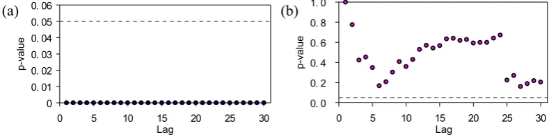
Figure 9 McLeod-Li test for the residuals from (a) ARMA(20,1) model for daily flow and

(b) AR(4) model for monthly flow

(a)

(b)

(a)

(b)

(a) (b)

Fig. 7. Ljung-Box lack-of-fit tests for (a) the ARMA(20,1) model for daily flow and (b) the AR(4) model for monthly flow.

20

0 0. 05 0. 1 0. 15 0. 2 0. 25 0. 3

21 26 31 36

Lag

p-val

u

e

0 0. 2 0. 4 0. 6 0. 8 1

4 6 8 10 12 14 16 18 20

Lag

p-val

u

e

Figure 7 Ljung-Box lack-of-fit tests for (a) ARMA(20,1) model for daily flow and (b) AR(4)

0 100 200 300 Lag

0.

0

.1

0.

2

AC

F

0 2 4 6 8 10 12 Lag

0.0

0

.1

0

.2

AC

F

0 0. 01 0. 02 0. 03 0. 04 0. 05 0. 06

0 5 10 15 20 25 30 Lag

p-value

0. 0 0. 1 0. 2 0. 3 0. 4 0. 5 0. 6 0. 7 0. 8

0 5 10 15 20 25 30 Lag

p-value

Figure 9 McLeod-Li test for the residuals from (a) ARMA(20,1) model for daily flow and

(b) AR(4) model for monthly flow

(a)

(b)

(a)

(b)

(a) (b)

Fig. 8. ACFs of the squared residuals from (a) the ARMA(20,1) model for daily flow and (b) the AR(4) model for monthly flow at Tangnaihai.

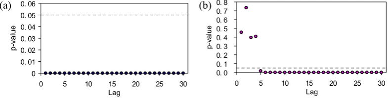
where N is the sample size, and rˆ_k2 is the squared sample autocorrelation of squared residual series at lagk. Under the null hypothesis of a linear generating mechanism for the data, namely, no ARCH effect in the data, the test statistic is asymptoticallyχ2(L)distributed. Figure 9 shows the results of the McLeod-Li test for daily and monthly flow. It illus-trates that the null hypothesis of no ARCH effect is rejected for both daily and monthly flow series.

3.3 Engle’s Lagrange Multiplier test for the ARCH effect Since the ARCH model has the form of an autoregres-sive model, Engle (1982) proposed the Lagrange Multiplier (LM) test, in order to test for the existence of ARCH be-haviour based on the regression. The test statistic is given by TR2, where R is the sample multiple correlation coef-ficient computed from the regression of ε_t2 on a constant andε2_t₋₁,. . . ,ε_t2−q, andT is the sample size. Under the null hypothesis that there is no ARCH effect, the test statistic is asymptotically distributed as chi-square distribution with

q degrees of freedom. As Bollerslev (1986) suggested, it should also have power against GARCH alternatives.

Figure 10 shows Engle’s LM test results for the residu-als from the ARMA(20,1) model for daily flow and from the AR(4) model for monthly flow. The results also firmly in-dicate the existence of an ARCH effect in both the residual series.

One point that should be noticed is that although Figs. 8b, 9b and 10b show that for monthly flow, autocorrelations at

lags less than 4 are removed by the AR(4) model, when we take autocorrelations at longer lags into consideration, sig-nificant autocorrelations remain and the null hypothesis of no ARCH effect is rejected. Because it is required for the McLeod-Li test to use sufficiently largeL, namely, a suf-ficient number of autocorrelations to calculate the Ljung-Box statistic (typically around 20), we still consider that the monthly flow has the ARCH effect.

On the whole, evidences are clear with the McLeod-Li test and Engle’s LM test about the existence of conditional het-eroskedasticity in the residual series from linear models fitted to the logarithmized and deseasonalized daily and monthly streamflow processes of the upper Yellow River at Tangnai-hai.

4 Discussion of the causes of ARCH effects and inade-quacy of commonly used seasonal time series models 4.1 Causes of ARCH effects in the residuals from

ARMA-type models for daily and monthly flow

(6)

20

0

0. 05 0. 1 0. 15 0. 2 0. 25 0. 3

21 26 31 36

Lag

p-val

u

e

0 0. 2 0. 4 0. 6 0. 8 1

4 6 8 10 12 14 16 18 20

Lag

p-val

u

e

Figure 7 Ljung-Box lack-of-fit tests for (a) ARMA(20,1) model for daily flow and (b) AR(4)

0 100 200 300

Lag

0.

0

.1

0.

2

AC

F

0 2 4 6 8 10 12

Lag

0.0

0

.1

0

.2

AC

F

0 0. 01 0. 02 0. 03 0. 04 0. 05 0. 06

0 5 10 15 20 25 30

Lag

p-value

0. 0 0. 1 0. 2 0. 3 0. 4 0. 5 0. 6 0. 7 0. 8

0 5 10 15 20 25 30

Lag

p-value

Figure 9 McLeod-Li test for the residuals from (a) ARMA(20,1) model for daily flow and

(b) AR(4) model for monthly flow

(a)

(b)

(a)

(b)

(a) (b)

Fig. 9. McLeod-Li test for the residuals from (a) the ARMA(20,1) model for daily flow and (b) the AR(4) model for monthly flow.

21

0

0. 01 0. 02 0. 03 0. 04 0. 05 0. 06

0 5 10 15 20 25 30

Lag

p-value

0. 0 0. 1 0. 2 0. 3 0. 4 0. 5 0. 6 0. 7 0. 8

0 5 10 15 20 25 30

Lag

p-value

Figure 10 Engle’s LM test for residuals from (a) ARMA(20,1) model for daily flow and

0 0.1 0.2 0.3 0.4

0 60 120 180 240 300 360 Day

SD

0 0. 2 0. 4 0. 6 0. 8 1

0 3 6 9 12

Month

SD

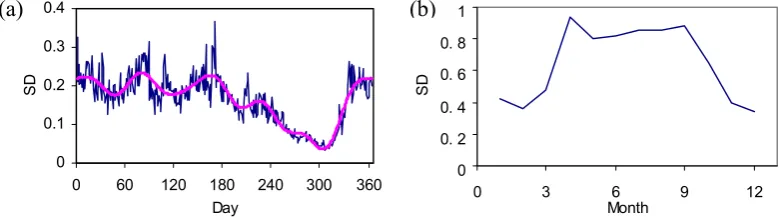
Figure 11 Seasonal standard deviations (SD) of the residuals form (a) ARMA(20,1) model for

daily flow and (b) AR(4) model for monthly flow

(Note: the smoothed line in Figure 11(a) is given by the first 8 Fourier harmonics of the

seasonal SD series.)

0 100 200 300

Lag

0

.0

0.1

0.

2

0

.3

AC

F

0 5 10

Lag

0.

0

.1

0.

2

AC

F

Figure 12 ACFs of squared seasonally standardized residuals from (a) ARMA(20,1) model

for daily flow and (b) AR(4) model for monthly flow

(a)

(b)

(a) (b)

(a)

(b)

Fig. 10. Engle’s LM test for residuals from (a) the ARMA(20,1) model for daily flow and (b) the AR(4) model for monthly flow.

the residual series from linear models with seasonal standard deviations of the residuals first, then look at the standard-ized series to check whether seasonal variances can explain ARCH effects.

Seasonal standard deviations of the residual series from the ARMA(20,1) model for daily flow and the AR(4) model for monthly flow are calculated and shown in Figs. 11a and 11b. They are used to standardize the residual series from the ARMA(20,1) model and the AR(4) model. Figure 12 shows the ACFs of the squared standardized residual series of daily and monthly flow. It is illustrated that, after sea-sonal standardized autocorrelation, as well as the seasea-sonality in the squared standardized residual series for monthly flow is basically removed (Fig. 12b), the significant autocorrela-tion still exists in the squared standardized residual series for daily flow (Fig. 12a), despite the fact that the autocorrela-tions are significantly reduced compared with Fig. 8a and the seasonality in the ACF structure is removed. This means that the seasonality, as well as the autocorrelation in the squared residuals from the AR model of monthly flow series is basi-cally caused by seasonal variances. But seasonal variances only explain partly the autocorrelation in the squared residu-als of daily flow series.

The residual series of daily flow and monthly flow stan-dardized by seasonal standard deviation are also tested for ARCH effects with the McLeod-Li test and Engle’s LM test. Figure 13 shows that the seasonally standardized residual series of daily flow still cannot pass the LM test (Fig. 13a), whereas the seasonally standardized residual se-ries of monthly flow pass the LM test with high p-values (Fig. 13b). The McLeod-Li test gives similar results.

From the above analyses, it is clear that the ARCH effect is fully caused by seasonal variances for monthly flow, but only partly for daily flow. Other causes, besides the seasonal vari-ation in variance, of the ARCH effect in daily flow may in-clude the perturbations of the temperature fluctuations which is an influential factor for snowmelt, as well as evapotran-spiration, and the precipitation variation which is the domi-nant factor for streamflow processes. As reported by Miller (1979), when modelling a daily average streamflow series, the residuals from a fitted AR(4) model signaled white-noise errors, but the squared residuals signaled bilinearity. When precipitation covariates were included in the model, Miller found that neither the residuals nor the squared residuals sig-naled any problems. While we agree that the autocorrela-tion existing in the squared residuals is basically caused by a precipitation process, we want to show that the autocorre-lation in the squared residuals can be well described by an ARCH model, which is very close to the bilinear model (En-gle, 1982).

4.2 Inadequacy of commonly used seasonal time series models for modelling streamflow processes

As mentioned in Sect. 3.1, SARIMA models, deseasonal-ized ARMA models and periodic models are commonly used to model hydrologic processes (Hipel and McLeod, 1994). Given a time series (xt), the general form of SARIMA model, denoted by SARIMA(p,d,q)×(P,D,Q)S, is

φ (B)8(Bs)∇d∇D

(7)

21

0 0. 01 0. 02 0. 03 0. 04 0. 05 0. 06

0 5 10 15 20 25 30 Lag

p-value

0. 0 0. 1 0. 2 0. 3 0. 4 0. 5 0. 6 0. 7 0. 8

0 5 10 15 20 25 30 Lag

p-value

Figure 10 Engle’s LM test for residuals from (a) ARMA(20,1) model for daily flow and

0 0.1 0.2 0.3 0.4

0 60 120 180 240 300 360 Day

SD

0 0. 2 0. 4 0. 6 0. 8 1

0 3 6 9 12

Month

SD

0 100 200 300 Lag

0

.0

0.1

0.

2

0

.3

AC

F

0 5 10

Lag

0.

0

.1

0.

2

AC

F

for daily flow and (b) AR(4) model for monthly flow

(a)

(b)

(a) (b)

(a)

(b)

Fig. 11. Seasonal standard deviations (SD) of the residuals from (a) the ARMA(20,1) model for daily flow and (b) the AR(4) model for

monthly flow (note: the smoothed line in (a) is given by the first 8 Fourier harmonics of the seasonal SD series).

21

0 0. 01 0. 02 0. 03 0. 04 0. 05 0. 06

0 5 10 15 20 25 30 Lag

p-value

0. 0 0. 1 0. 2 0. 3 0. 4 0. 5 0. 6 0. 7 0. 8

0 5 10 15 20 25 30 Lag

p-value

Figure 10 Engle’s LM test for residuals from (a) ARMA(20,1) model for daily flow and

0 0.1 0.2 0.3 0.4

0 60 120 180 240 300 360 Day

SD

0 0. 2 0. 4 0. 6 0. 8 1

0 3 6 9 12

Month

SD

0 100 200 300 Lag

0

.0

0.1

0.

2

0

.3

AC

F

0 5 10

Lag

0.

0

.1

0.

2

AC

F

for daily flow and (b) AR(4) model for monthly flow

(a)

(b)

(a) (b)

(a)

(b)

Fig. 12. ACFs of squared seasonally standardized residuals from (a) the ARMA(20,1) model for daily flow and (b) the AR(4) model for

monthly flow.

and2(Bs)of ordersP andQrepresent the seasonal autore-gressive and moving average components;∇d=(1−B)d and ∇D

S =(1−Bs)Dare the ordinary and seasonal difference com-ponents.

The general form of the ARMA(p,q) model fitted to de-seasonalized series is

φ (B)xt =θ (B)εt. (4)

From the model equations we know that although the sea-sonal variation in the variance present in the original time series is basically dealt with well by the deseasonalized ap-proach, the seasonal variation in variance in the residual se-ries is not considered by either of the two models, because in both cases the innovation seriesεtis assumed to be i.i.d.N(0,

σ2). Therefore, both SARIMA models and deseasonalized models cannot capture the ARCH effect that we observed in the residual series.

In contrast, the periodic model, which is basically a group of ARMA models fitted to separate seasons, allows for sea-sonal variances in not only the original series but also the residual series. Taking the special case PAR(p) model (pe-riodic autoregressive model of order p) as an example of a PARMA model, given a hydrological time seriesxn,s, in whichndefines the year andsdefines the season (could

rep-resent a day, week, month or season), we have the following PAR(p) model (Salas, 1993):

xn,s =µs + p X j=1

φj,s(xv,s−j−µs−j)+εn,s, (5)

whereεn,sis an uncorrelated normal variable with mean zero and variance σ2_s. For daily streamflow series, to make the model parsimonious, we can cluster the days in the year into several groups and fit separate AR models to separate groups (Wang et al., 2004). Periodic models would per-form better than the SARIMA model and the deseasonal-ized ARMA model for capturing the ARCH effect, because it takes season-varying variances into account. However, as analyzed in Sect. 4.1, while considering seasonal vari-ances could be sufficient for describing the ARCH effect in monthly flow series because the ARCH effect in monthly flow series is fully caused by seasonal variances, it is still insufficient to fully capture the ARCH effect in daily flow series.

(8)

22

0 0. 01 0. 02 0. 03 0. 04 0. 05 0. 06

0 5 10 15 20 25 30 Lag

p-value

0. 0 0. 2 0. 4 0. 6 0. 8 1. 0

0 5 10 15 20 25 30 Lag

p-value

Figure 13 Engle’s LM test for seasonally standardized residuals from (a) ARMA(20,1) model

for daily flow and (b) from AR(4) model for monthly flow

0 20 40 60 80 100

Lag

0

.00

0.0

5

0.

10

0.1

5

0.

20

P

ar

tia

l AC

F

Figure 14 PACF of the squared seasonally starndardized residual series from ARMA(20,1)

for daily flow

0 200 400 600 800 1000

-4

-2

0246

Day

Res

id

uals

0 200 400 600 800 1000

1.

0

1

.5

2.

0

2

.5

3.

0

Day

Con

d

itional

st

andard

devi

a

tion

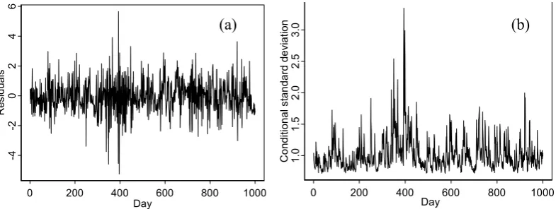
Figure 15 A segment of (a) the seasonally standardized residuals from ARMA(20,1) and (b)

its corresponding conditional standard deviation sequence estimated with ARCH(21) model

(a) (b)

Fig. 13. Engle’s LM test for seasonally standardized residuals from (a) the ARMA(20,1) model for daily flow and (b) from the AR(4) model

for monthly flow.

22

0 0. 01 0. 02 0. 03 0. 04 0. 05 0. 06

0 5 10 15 20 25 30

Lag

p-value

0. 0 0. 2 0. 4 0. 6 0. 8 1. 0

0 5 10 15 20 25 30

Lag

p-value

Figure 13 Engle’s LM test for seasonally standardized residuals from (a) ARMA(20,1) model

0 20 40 60 80 100

Lag

0

.00

0.0

5

0.

10

0.1

5

0.

20

P

ar

tia

l AC

F

for daily flow

0 200 400 600 800 1000

-4

-2

0246

Day

Res

id

uals

0 200 400 600 800 1000

1.

0

1

.5

2.

0

2

.5

3.

0

Day

Con

d

itional

st

andard

devi

a

tion

its corresponding conditional standard deviation sequence estimated with ARCH(21) model

(a) (b)

Fig. 14. PACF of the squared seasonally starndardized residual

se-ries from ARMA(20,1) for daily flow.

5 Modelling the daily steamflow with ARMA-GARCH error model

5.1 Model building

Weiss (1984) proposed ARMA models with ARCH errors. This approach is adopted and extended by many researchers for modelling economic time series (e.g. Hauser and Kunst, 1998; Karanasos, 2001). In the field of geo-sciences, Tol (1996) fitted a GARCH model for the conditional variance and the conditional standard deviation, in conjunction with an AR(2) model for the mean, to model daily mean tempature. In this paper, we propose to use ARMA-GARCH er-ror (or, for notation convenience, called ARMA-GARCH) model for modelling daily streamflow processes.

The ARMA-GARCH model may be interpreted as a com-bination of an ARMA model which is used to model mean behaviour, and an ARCH model which is used to model the ARCH effect in the residual series from the ARMA model. The ARMA model has the form as in Eq. (4). The

GARCH(p,q)model has the form (Bollerslev, 1986) 

 

εt|ψt−1∼N (0, ht)

ht =α0+ q P i=1

αiε_t2−i + p P i=1

βiht−i , (6)

where,εt denotes a real-valued discrete-time stochastic pro-cess, and ψt the available information set, p ≥0, q >0,

α0 >0,αi ≥0,βi ≥0. Whenp=0, the GARCH(p,q)model reduces to the ARCH(q)model. Under the GARCH(p, q) model, the conditional variance of εt, ht, depends on the squared residuals in the previousqtime steps, and the condi-tional variance in the previousptime steps. Since GARCH models can be treated as ARMA models for squared residu-als, the order of GARCH can be determined with the method for selecting the order of ARMA models, and traditional model selection criteria, such as Akaike information criterion (AIC) and Bayesian information criterion (BIC), can also be used for selecting models. The unknown model parameters

αi (i= 0,· · ·,q)andβj (j= 1,· · ·,p)can be es-timated using (conditional) maximum likelihood estimation (MLE). Estimates of the conditional standard deviationh1_t/2

are also obtained as a side product with the MLE method. When there is obvious seasonality present in the residuals (as in the case of daily streamflow at Tangnaihai), to preserve the seasonal variances in the residuals, instead of fitting the ARCH model to the residual series directly, we fit the ARCH model to the seasonally standardized residual series, which is obtained by dividing the residual series by seasonal stan-dard deviations (i.e. daily stanstan-dard deviations for daily flow). Therefore, the general ARMA-GARCH model with seasonal standard deviations we propose here has the following form

  

φ (B)xt =θ (B)εt

εt =σszt, zt∼N (0, ht)

ht =α0+ q P i=1

αiz2_t−i+ p P i=1

βiht−i

, (7)

whereσsis the seasonal standard deviation ofεt,sis the sea-son number depending on which seasea-son the timetbelongs to. For daily series,sranges from 1 to 366. Other notations are the same as in Eqs. (4) and (6).

(9)

22

0 0. 01 0. 02 0. 03 0. 04 0. 05 0. 06

0 5 10 15 20 25 30 Lag

p-value

0. 0 0. 2 0. 4 0. 6 0. 8 1. 0

0 5 10 15 20 25 30 Lag

p-value

Figure 13 Engle’s LM test for seasonally standardized residuals from (a) ARMA(20,1) model

0 20 40 60 80 100 Lag

0

.00

0.0

5

0.

10

0.1

5

0.

20

P

ar

tia

l AC

F

for daily flow

0 200 400 600 800 1000

-4

-2

0246

Day

Res

id

uals

0 200 400 600 800 1000

1.

0

1

.5

2.

0

2

.5

3.

0

Day

Con

d

itional

st

andard

devi

a

tion

its corresponding conditional standard deviation sequence estimated with ARCH(21) model

(a) (b)

Fig. 15. A segment of (a) the seasonally standardized residuals from ARMA(20,1) and (b) its corresponding conditional standard deviation

sequence estimated with the ARCH(21) model.

23

0 20 40 60 80 100 Lag

0.

0

0.

1

0.

2

AC

F

0 20 40 60 80 100 Lag

0.0

0

.1

0.2

AC

F

Figure 16 ACFs of (a) the standardized residuals and (b) squared standardized residuals from

ARMA(20,1)-ARCH(21) model. The standardization is accomplished by dividing the

seasonally standardized residuals from ARMA(20,1) by the conditional standard deviation

estimated with ARCH(21).

0 20 40 60 80 100 Lag

0.0

0.1

0

.2

AC

F

0 20 40 60 80 100 Lag

0.

0

0.

1

0.

2

Par

tial

AC

F

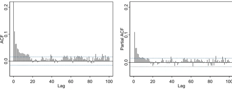
Figure 17 ACF and PACF of seasonally standardized residuals from ARMA(20,1) model

0 20 40 60 80 100 Lag

0.

0

.1

0

.2

AC

F

0 20 40 60 80 100 Lag

0.0

0.1

0.2

AC

F

Figure 18 ACFs of (a) the second-residuals and (b) the squared second-residuals from the

ARMA(20,1)-AR(16) model

(a) (b)

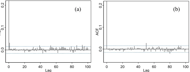
Fig. 16. ACFs of (a) the standardized residuals and (b) squared standardized residuals from the ARMA(20,1)-ARCH(21) model. The

standardization is accomplished by dividing the seasonally standardized residuals from ARMA(20,1) by the conditional standard deviation estimated with ARCH(21).

1. Logarithmize and deseasonalize the original flow series; 2. Fit an ARMA model to the logarithmized and

deseason-alized flow series;

3. Calculate seasonal standard deviations of the residuals obtained from ARMA model, and seasonally standard-ize the residuals with the first 8 Fourier harmonics of the seasonal standard deviations;

4. Fit a GARCH model to the seasonally standardized residual series.

For forecasting and simulation, inverse transformation (in-cluding logarithmization and deseasonalization) is needed. When forecasting, the ARMA part of the ARMA-GARCH model forecasts future mean values of the underlying time se-ries following the traditional approach for ARMA prediction, whereas the GARCH part gives forecasts of future volatility, especially over short horizons.

Following the above-mentioned steps, a preliminary ARMA-GARCH model is fitted to the daily streamflow series at Tangnaihai. The ACF and PACF structure of

the squared seasonally standardized residuals are shown in Fig. 12a and Fig. 14, respectively. According to the AIC, as well as the ACF and PACF structure, a GARCH(0,21) model, i.e. ARCH(21) model, which has the smallest AIC value is selected. Therefore, the prelimilary ARMA-GARCH model fitted to the daily streamflow series at Tangnaihai is com-posed of an ARMA(20,1) model and an ARCH(21) model. The model is constructed with statistics software S-Plus (Zivot and Wang, 2003).

5.2 Model diagnostic and modification

If the ARMA-GARCH model is successful in modelling the serial correlation structure in the conditional mean and con-ditional variance, then there should be no autocorrelation left in both the residuals and the squared residuals standardized by the estimated conditional standard deviation.

(10)

23

0 20 40 60 80 100

Lag

0.

0

0.

1

0.

2

AC

F

0 20 40 60 80 100 Lag

0.0

0

.1

0.2

AC

F

Figure 16 ACFs of (a) the standardized residuals and (b) squared standardized residuals from

0 20 40 60 80 100 Lag

0.0

0.1

0

.2

AC

F

0 20 40 60 80 100 Lag

0.

0

0.

1

0.

2

Par

tial

AC

F

Figure 17 ACF and PACF of seasonally standardized residuals from ARMA(20,1) model

0 20 40 60 80 100 Lag

0.

0

.1

0

.2

AC

F

0 20 40 60 80 100 Lag

0.0

0.1

0.2

AC

F

Figure 18 ACFs of (a) the second-residuals and (b) the squared second-residuals from the

(a) (b)

Fig. 17. ACF and PACF of seasonally standardized residuals from the ARMA(20,1) model.

23

0 20 40 60 80 100

Lag

0.

0

0.

1

0.

2

AC

F

0 20 40 60 80 100 Lag

0.0

0

.1

0.2

AC

F

Figure 16 ACFs of (a) the standardized residuals and (b) squared standardized residuals from

0 20 40 60 80 100 Lag

0.0

0.1

0

.2

AC

F

0 20 40 60 80 100 Lag

0.

0

0.

1

0.

2

Par

tial

AC

F

Figure 17 ACF and PACF of seasonally standardized residuals from ARMA(20,1) model

0 20 40 60 80 100 Lag

0.

0

.1

0

.2

AC

F

0 20 40 60 80 100 Lag

0.0

0.1

0.2

AC

F

Figure 18 ACFs of (a) the second-residuals and (b) the squared second-residuals from the

(a) (b)

Fig. 18. ACFs of (a) the second-residuals and (b) the squared second-residuals from the ARMA(20,1)-AR(16) model.

the ARMA(20,1) model by dividing it by the estimated conditional standard deviation sequence. The autocorrela-tions of the standardized residuals and squared standardized residuals are plotted in Fig. 16. It is shown that although there is no autocorrelation left in the squared standardized residuals, which means that the ARCH effect has been re-moved (Fig. 16b), however, in the non-squared standardized residuals of daily flow significant autocorrelation remains (Fig. 16a).

Because the GARCH model is designed to deal with the conditional variance behavior, rather than mean behavior, the autocorrelation in the non-squared residual series must arise from the seasonally standardized residuals obtained in step 3 of the ARMA-GARCH model building procedure. Therefore we revisit the seasonally standardized residuals. It is found that although the residuals from the ARMA(20,1) model present no obvious autocorrelation as shown in Fig. 6a, weak but significant autocorrelations in the residuals are revealed after the residuals are seasonally standardized, as shown by the ACF and PACF in Fig. 17. We refer to this weak autocor-relation as the hidden weak autocorautocor-relation.

The mechanism underlying such weak autocorrelation is not clear yet. Similar phenomena are also found for some other daily streamflow processes (such as the daily

stream-flow of the Umpqua River near Elkton and the Wisconsin River near Wisconsin Dells, available on the USGS website http://water.usgs.gov/waterwatch), which have strong sea-sonality in the ACF structures of their original series, as well as their residual series. To handle the problem of the weak correlations, an additional ARMA model is needed to model the mean behaviour in the seasonally standardized residuals, and a GARCH is then fitted to the residuals from this ad-ditional ARMA model. Therefore, we obtain an extended version of the model in Eq. (7) as

      

φ (B)xt =θ (B)εt

εt =σsyt

φ0(B)yt =θ0(B)zt, zt∼N (0, ht)

ht =α0+ q P i=1

αiz2t−i+ p P i=1

βiht−i

, (8)

where yt is the seasonally standardized residuals from the first ARMA model,zt is the residuals (for notation conve-nience, we call it second-residuals) from the second ARMA model fitted toyt.

(11)

se-W. Wang et al.: Testing and modelling autoregressive conditional heteroskedasticity 65

24

0 20 40 60 80 100 Lag

0.0

0

.1

0.2

AC

F

0 20 40 60 80 100 Lag

0.0

0

.1

0.2

AC

F

Figure 19 ACFs of the (a) standardized residuals and (b) squared standardized

second-residuals from ARMA(20,1)-AR(16)-ARCH(21) model. The second-second-residuals are obtained

from AR(16) fitted to the seasonally standardized residuals form ARMA(20,1).

0 0. 2 0. 4 0. 6 0. 8 1

0 5 10 15 20 25 30 Lag

p-v

al

ue

Figure 20 Engle’s LM test for the standardized second-residuals from the

ARMA(20,1)-AR(16)-ARCH(21) model

(a) (b)

Fig. 19. ACFs of (a) the standardized second-residuals and (b) the squared standardized second-residuals from the

ARMA(20,1)-AR(16)-ARCH(21) model. The second-residuals are obtained from AR(16) fitted to the seasonally standardized residuals from ARMA(20,1).

ries from this AR(16) model. The autocorrelations of the second-residual series and the squared second-residual series from the ARMA(20,1)-AR(16) combined model are shown in Fig. 18. From visual inspection, we find that no autocorre-lation is left in the second-residual series, but there is strong autocorrelation in the squared second-residual series which indicates the existence of an ARCH effect.

Because the squared second-residual series has similar ACF and PACF stucture to the seasonally standardized resid-uals from the ARMA(21,0) model, the same structure of the GARCH model, i.e. an ARCH(21) model, is fitted to the second-residual series. Therefore, the ultimate ARMA-GARCH model fitted to the daily streamflow at Tangnai-hai is ARMA(20,1)-AR(16)-ARCH(21), composed of an ARMA(20,1) model fitted to logarithmized and deseasonal-ized series, an AR(16) model fitted to the seasonally stan-dardized residuals from the ARMA(20,1) model, and an ARCH(21) model fitted to the second-residuals from the AR(16) model.

We standardize the second-residual series with the con-ditional standard deviation sequence obtained with the ARCH(21) model. The autocorrelations of the standard-ized residuals and the squared standardstandard-ized second-residuals are shown in Fig. 19. Compared with Fig. 16, the autocorrelations are basically removed for both the squared and non-squared series, although the autocorrelation at lag 1 of the standardized second-residuals slightly exceeds the 5% significance level. The McLeod-Li test and the LM-test (shown in Fig. 20) for standardized second-residuals also confirm that the ARCH(21) model fits the second-residual se-ries well. The small lag-1 autocorrelation in the standardized second-residual series (shown in Fig. 19) is a hidden autocor-relation covered by conditional heteroskedasticity. This au-tocorrelation can be further modeled with another AR model, but because the autocorrelation is very small, it could be ne-glected.

24

0 20 40 60 80 100

Lag

0.0

0

.1

0.2

AC

F

0 20 40 60 80 100

Lag

0.0

0

.1

0.2

AC

F

Figure 19 ACFs of the (a) standardized residuals and (b) squared standardized

second-residuals from ARMA(20,1)-AR(16)-ARCH(21) model. The second-second-residuals are obtained

from AR(16) fitted to the seasonally standardized residuals form ARMA(20,1).

0 0. 2 0. 4 0. 6 0. 8 1

0 5 10 15 20 25 30

Lag

p-v

al

ue

Figure 20 Engle’s LM test for the standardized second-residuals from the

ARMA(20,1)-AR(16)-ARCH(21) model

(a) (b)

Fig. 20. Engle’s LM test for the standardized second-residuals from

the ARMA(20,1)-AR(16)-ARCH(21) model.

6 Conclusions

The nonlinear mechanism conditional heteroskedasticity in hydrologic processes has not received much attention in the literature so far. Modelling data with time varying condi-tional variance could be attempted in various ways, includ-ing nonparametric and semi-parametric approaches (see Lall, 1995; Sankarasubramanian and Lall, 2003). A parametric approach with ARCH model is proposed in this paper to de-scribe the conditional variance behavior. ARCH-type mod-els which originate from econometrics can provide accurate forecasts of variances. As a consequence, they can be ap-plied to such diverse fields as water management risk anal-ysis, prediction uncertainty analysis and streamflow series simulation.

(12)

66 W. Wang et al.: Testing and modelling autoregressive conditional heteroskedasticity PARMA model is enough for monthly flow by considering

season-dependent variances. Therefore, to fully capture the ARCH effect, as well as the seasonal variances inspected in the residuals from linear ARMA models fitted to the daily flow series, the ARMA-GARCH error model with seasonal standard deviations is proposed. The ARMA-GARCH model is basically a combination of an ARMA model which is used to model mean behaviour, and a GARCH model to model the ARCH effect in the residuals from the ARMA model. To preserve the seasonal variation in variance in the residuals, the ARCH model is not fitted to the residual series directly, but to the seasonally standardized residuals. Therefore, an important feature of the ARMA-GARCH model is that the unconditional seasonal variance of the process is seasonally constant but the conditional variance is not. To resolve the problem of the weak hidden autocorrelation revealed after the residuals are seasonally standarized, the ARMA-GARCH model is extended by applying an additional ARMA model to model the mean behaviour in the seasonally standard-ized residual series. With such a modified ARMA-GARCH model, the daily streamflow series is well-fitted.

Because the ARCH effect in daily streamflow mainly arises from daily variations in temperature and precipita-tion, and given that we have reasonably good skill in pre-dicting weather two to three days in advance (for example, see http://weather.gov/rivers tab.php), the use in developing an ARMA-GARCH model would be limited. However, be-cause (1) on the one hand, the relationship between runoff and rainfall and temperature is hard to capture precisely by any model so far; (2) on the other hand, usually there are not enough rainfall data available to fully capture the rain-fall spatial pattern, especially for remote areas, such as Ti-bet Plateau, and (3) the accuracy of the weather forecasts for these areas are very limited, the ARCH effect cannot be fully removed even after limited rainfall data and temperature data are included in the model. Therefore, the ARMA-GARCH model would be a very useful addition in terms of statistical modelling of daily streamflow processes for the hydrological community.

Acknowledgements. We are very grateful to I. McLeod and an

anonymous reviewer. Their comments, especially the detailed

comments from the anonymous reviewer, are very helpful to improve the paper considerably.

Edited by: B. Sivakumar

Reviewed by: I. McLeaod and another referee

References

Bollerslev, T.: Generalized Autoregressive Conditional

Het-eroscedasticity, Journal of Econometrics, 31, 307–327, 1986. Box, G. E. P. and Jenkins, J. M.: Time series analysis: Forecasting

and control, San Francisco, Holden-Day, 1976.

Brock, W. A., Dechert, W. D., Scheinkman, J. A., and LeBaron, B.: A test for independence based on the correlation dimension, Econ. Rev., 15, 3, 197–235, 1996.

Engle, R.: Autoregressive conditional heteroscedasticity with esti-mates of the variance of UK inflation, Econometrica, 50, 987– 1008, 1982.

Granger, C. W. J. and Andersen, A. P.: An introduction to bilin-ear time series models, G¨ottingen, Vandenhoeck and Ruprecht, 1978.

Hipel, K. W. and McLeod, A. I.: Time series modelling of water resources and environmental systems, Elsvier, Amsterdam, 1994. Karanasos, M.: Prediction in ARMA models with GARCH-in-mean effects, Journal of Time Series Analysis, 22, 555–78, 2001. Lall, U.: Recent advance in nonparametric function estimation – hydrologic application, Reviews of Geophysics, 33, 1093–1102, 1995.

Livina, V., Ashkenazy, Y., Kizner, Z., Strygin, V., Bunde, A., and Havlin, S.: A stochastic model of river discharge fluctuations, Physica A, 330, 283–290, 2003.

Ljung, G. M. and Box, G. E. P.: On a measure of lack of fit in time series models, Biometrika, 65, 297–303, 1978.

McLeod, A. I. and Li, W. K.: Diagnostic checking ARMA time series models using squared residual autocorrelations, Journal of Time Series Analysis, 4, 269–273, 1983.

Miller, R. B.: Book review on “An Introduction to Bilinear Time Series Models” by Granger, C. W. and Andersen, A. P., J. Amer. Statist. Ass., 74, 927, 1979.

Hauser, M. A. and Kunst, R. M.: Fractionally Integrated Models With ARCH Errors: With an Application to the Swiss 1-Month Euromarket Interest Rate, Review of Quantitative Finance and Accounting, 10, 95–113, 1998.

Salas, J. D.: Analysis and modelling of hydrologic time series. In: Handbook of Hydrology, edited by Maidment, D. R., McGraw-Hill, 19.1–19.72, 1993.

Sankarasubramanian, A. and Lall, U.: Flood quantiles in a chang-ing climate: Seasonal forecasts and causal relations, Water Re-sources Research, 39, 5, Art. No. 1134, 2003.

Tol, R. J. S.: Autoregressive conditional heteroscedasticity in daily temperature measurements, Environmetrics, 7, 67–75, 1996. Wang, W., Van Gelder, P. H. A. J. M., and Vrijling, J. K.:

Peri-odic autoregressive models applied to daily streamflow. In: 6th International Conference on Hydroinformatics, edited by Liong, S. Y., Phoon, K. K. and Babovic, V., Singapore, World Scientific, 1334–1341, 2004.

Weiss, A. A.: ARMA models with ARCH errors, Journal of Time Series Analysis, 5, 129–143, 1984.

http://water.usgs.gov/waterwatch),

http://weather.gov/rivers tab.php)