www.nonlin-processes-geophys.net/17/615/2010/ doi:10.5194/npg-17-615-2010
© Author(s) 2010. CC Attribution 3.0 License.
Nonlinear Processes
in Geophysics
Characterizing the structure of nonlinear systems using gradual
wavelet reconstruction
C. J. Keylock
Department of Civil and Structural Engineering, University of Sheffield, Sheffield, UK
Received: 11 November 2009 – Revised: 2 September 2010 – Accepted: 11 October 2010 – Published: 16 November 2010
Abstract. In this paper, classical surrogate data methods for testing hypotheses concerning nonlinearity in time-series data are extended using a wavelet-based scheme. This gives a method for systematically exploring the properties of a signal relative to some metric or set of metrics. A signal continuum is defined from a linear variant of the original signal (same histogram and approximately the same Fourier spectrum) to the exact replication of the original signal. Surrogate data are generated along this continuum with the wavelet trans-form fixing in place an increasing proportion of the proper-ties of the original signal. Eventually, chaotic or nonlinear behaviour will be preserved in the surrogates. The technique permits various research questions to be answered and ex-amples covered in the paper include identifying a threshold level at which signals or models for those signals may be considered similar on some metric, analysing the complexity of the Lorenz attractor, characterising the differential sensi-tivity of metrics to the presence of multifractality for a turbu-lence time-series, and determining the amplitude of variabil-ity of the H¨older exponents in a multifractional Brownian motion that is detectable by a calculation method. Thus, a wide class of analyses of relevance to geophysics can be un-dertaken within this framework.
1 Introduction
Because of the wide ranging occurrence and varied nature of nonlinearity in geophysical time series (Johnson et al., 2005; Khan et al., 2005; Roux et al., 2009), gaining an un-derstanding of the sources of any nonlinearity is an impor-tant topic. The presence of nonlinearity can be tested by
ap-Correspondence to: C. J. Keylock ([email protected])
plying some metric, such as time asymmetry (Schreiber and Schmitz, 1997) or maximal Lyapunov exponent to a time se-ries of outputs from a system and comparing the response to surrogate data that are linear variants of the original signal. A test for any significant difference can be developed within this framework (Theiler et al., 1992; Schreiber and Schmitz, 1996). The intention of this paper is to pursue this matter in a new direction. The approach developed here moves away from the acceptance/rejection framework of the hypothesis test for nonlinearity to ask: How similar to the original data do the surrogates need to be to avoid rejection of the null hy-pothesis? From this, it is possible to develop new research questions within a surrogate data framework, such as:
– Which parts of the time series need to be identical be-tween the data and the surrogate in order to prevent the rejection of the null hypothesis (i.e. what are the most complicated parts of the original time series)?
– Does the range of values for a metric calculated for a set of surrogates that are not statistically different to the original data include the value of this metric for a model of that system (i.e. is the model validated)?
– Do different, but related nonlinear or chaotic time series exhibit differences in how similar their surrogates need to be to the original data to avoid rejecting the null hy-pothesis (i.e. are there differences in complexity of the series)?
Our approach, which we term Gradual Wavelet Recon-struction, permits these questions to be answered. This is illustrated by the examples presented in the final parts of the paper. Before this, we explain the gradual wavelet recon-struction approach, which requires us first to review briefly relevant literature on hypothesis testing for surrogate data in nonlinear science.
2 Hypothesis testing for nonlinear time series using surrogate data
The surrogate data methodology as proposed by Theiler et al. (1992) and enhanced by Schreiber and Schmitz (1996) is a common technique with applications in studies of river me-andering (Frascati and Lanzoni, 2010), ice core data (Kwas-niok and Lohmann, 2009), environmental turbulence (Basu et al., 2007; Keylock, 2009) and the magnetosphere (Pavlos et al., 1999), as well as other disciplines beyond geoscience, such as medicine (Mormann et al., 2005). Typically, one gen-erates surrogate data that are stochastic realisations from a Gaussian linear system with the same values and (to some error tolerance) Fourier spectrum as the original data and employs a metric to see if the observed time series is signifi-cantly different to the surrogates. For a two-tailed hypothesis test at a significance level,a, if the value of the metric for the original data is less than or greater than that for all of the
(2/a)−1 surrogate datasets then the null hypothesis that the original data is a realisation of a Gaussian linear process will be rejected.
An effective method for producing surrogate data that preserve the values and, to some error level, the Fourier spectrum of the original data is the Iterated Amplitude Ad-justed Fourier Transform (IAAFT) algorithm (Schreiber and Schmitz, 1996). Given a discrete time seriesgn,n=1,...,N
this algorithm proceeds as follows:
1. Store the squared amplitudes of the discrete Fourier transform ofgn(i.e.G2f= |P1Ngnei2π f n/N|2);
2. perform a random shuffle ofgnto givegn(0);
3. Subsequently, iterate a power spectrum step and a rank-order matching step ong(j )n as follows:
(a) Take the Fourier transform ofgn(j )and replace the
squared amplitudes with G2f, while retaining the phases. Given the initial random sort, this means that the spectrum should be preserved but with ran-dom phases. Invert the transformation with the am-plitudes replaced;
(b) Replace the values in the new seriesg(j )n by those in gnusing a rank-order matching process. This
pre-serves the set of original values in the dataset but deteriorates the quality of spectral matching, which explains why the Fourier amplitudes are only repli-cated approximately;
4. Repeat until a convergence criterion is fulfilled or any changes are too small to result in any re-ordering of the values.
The phase randomisation part of the algorithm will destroy temporal organisation in the original series that contributes to any nonlinearity, while the fact that the amplitudes of the spectrum are approximately preserved and the values of the original dataset are completely preserved mean that dif-ferences on some metric between the data and the surro-gates cannot be attributed to these sources, which could be sources of difference between two linear time-series. Hence, a significant difference implies, either the presence of some form of nonlinearity in the original data or that these data are sampled from a non-Gaussian, linear process. Subse-quently, this algorithm has been refined by groups such as Venema et al. (2006) who relaxed step 3(b), by imposing the values ofgnmore gradually in order to improve convergence.
The IAAFT algorithm was first implemented in the wavelet domain by Keylock (2006) using a Maximal Over-lap Discrete Wavelet Transform (MODWT), which is de-scribed in the Appendix to this paper. Because a wavelet transform is a time-frequency decomposition (see A1), the use of a single IAAFT results in the constrained randomi-sation of a time-series of wavelet coefficients representing one particular frequency band (or scale). Thus, withJ dif-ferent scales, performing an IAAFT at each scale, results in a full-randomisation of the wavelet coefficients. Be-cause the IAAFT algorithm does not alter the values for these coefficients, the wavelet power spectrum obtained from the MODWT (which is proportional to the variance of the wavelet coefficients) is unaffected by this transformation. The convergence of this method compared to the standard IAAFT and the enhanced method of Venema et al. (2006) was tested by Keylock (2008a), while the approach devel-oped in Keylock (2006) has subsequently sparked interest in other new ways for describing stationarity of time series (Borgnat and Flandrin, 2009, 2010).
Keylock (2007) presented a refinement to the earlier method, which still used the MODWT and the IAAFT, but fixed in place particular wavelet coefficients to provide a flex-ible means for designing surrogates. It is this algorithm that underpins gradual wavelet reconstruction, as is explained in the next section.
3 Gradual wavelet reconstruction
3.1 The algorithm
As established in the Appendix for the continuous wavelet transform and as stated for the MODWT, the square of the wavelet coefficients w2(j,k)/j2 is the energy func-tion of a time-series signal decomposed over different scales/frequencies,j, and positions along the time series, k
N=2J there will be a total ofk=1,...,N wavelet
coeffi-cients at each scale,j produced by the MODWT. The total energy content of the real-valued wavelet transformed signal is proportional to
E=
J
X
j=1
N
X
k=1
w2j,k (1)
and we defineρ as some chosen fraction ofE. If thewj,k2
are placed in aJ×N length vector in descending rank or-der, the smallest number ofwj,k2 required to attainρ can be determined by cumulating the squared wavelet coefficients until their sum as a fraction ofE attainsρ. We term these the fixed wavelet coefficients. The other coefficients are ran-domised as explained below. Hence,ρ provides a measure that can be used to vary the degree of similarity between the surrogates and original data (Keylock, 2007). Forρ=0 there are no fixed coefficients and the resulting surrogate will be similar to that obtained using the IAAFT. Trivially, forρ=1 all coefficients are fixed, no randomisation occurs and the surrogates and data are identical.
More formally, ifW∈R+is the set ofJ×N coefficients,
w2j,k, placed in descending rank order then, with 1≤n≤ (J×N )acting as an index forW, the set of fixed coefficients,
F⊆W, is given by the firstnelements ofW that fulfils the condition
Pn i=1w2i
E
≥ρ. Hence, the{w21,...,wn2} ∈F are the smallest number of coefficients that fulfils the energy pro-portion,ρE.
The algorithm for generating a surrogate data series using this approach may now be stated. This is an improved ver-sion of the algorithm given by Keylock (2007). The wavelet used in this paper is a Daubechies (1993) least-asymmetric wavelet with 16 vanishing moments for effective frequency localisation. The centre frequency (i.e. the frequency that maximises the Fourier transform of the modulus of the wavelet) is 0.6774 and the relation between scale,j, and the negative logarithm of the pseudo frequencies has a propor-tionality constant of 0.693. We made use of MATLAB and software accompanying Percival and Walden (2000), written by Charlie Cornish and available from WMTSA (2006) to implement the MODWT.
1. Choose a value forρ;
2. Perform a wavelet decomposition of the time series into aJ×N array using the MODWT and determine the fixed coefficients for thisρas explained, above; 3. For each wavelet scale, determine if any of the N
wavelet coefficients are to be fixed.
If they are not, apply the IAAFT algorithm to give a randomised realisation of the coefficients at this scale. If they are:
−2 0 2 4 6 8
u1
(m s
−1
)
10 10.2 10.4 10.6 10.8 11 11.2 11.4 11.6 −3
−2 −1 0 1 2 3
time (s)
u2
(m s
−1)
(a)
(b)
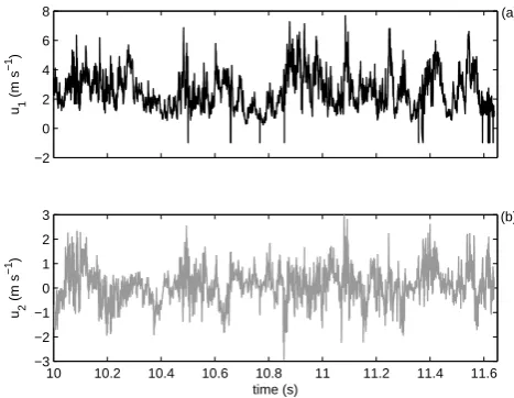
Fig. 1. Two perpendicular components of turbulent velocity data
(u1in black andu2in grey) obtained in a wind tunnel at 5000 Hz.
(a) Fit an exact interpolator through the fixed coeffi-cients and the end values; We used a piecewise cubic Hermitian polynomial method (Fritsch and Carlson, 1980);
(b) Add to this function the randomly shuffled, unfixed coefficients at this scale and use this as the starting point for the IAAFT algorithm;
(c) Run the IAAFT algorithm until convergence, reim-posing the fixed values in the correct positions at each rank-order matching step (see stage 3(b) of the IAAFT algorithm in Sect. 2);
4. Invert the wavelet transform to produce a new time se-ries of lengthN using the original approximation coef-ficients (which will be a constant for a stationary series if a full wavelet decomposition is undertaken, as is done throughout this paper) and the randomised detail coeffi-cients (see Eq. A9–A12 for an explanation of MODWT approximation and detail coefficients).
5. Because of a loss of the original values in the dataset from this operation (and a subsequent loss of matching of the power spectrum when they are imposed), re-peat stages (3) and (4) of the IAAFT algorithm to ensure convergence for the dataset as a whole.
Fixing in place more coefficients asρincreases means that the surrogates become progressively more similar to the data. Applying the IAAFT algorithm to each scale of the wavelet transform ensures that the coefficients have the appropriate autocorrelation function and can be reconstructed appropri-ately because they are a feasible realisation of a MODWT.
−0.5 0 0.5
w8,k
−0.5 0 0.5
w8,k
(0)
−0.5 0 0.5
w8,k
(1)
−0.5 0 0.5
w8,k
(cv)
−0.2 0 0.2
w8,k
(cv)
/
10.0 10.5 11.0 11.5
−0.2 0 0.2
time (s)
w8,k
(cv)
*/
(a)
(b)
(c)
(d)
(e)
(f)
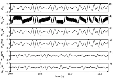
Fig. 2. Illustration of the surrogate generating algorithm foru1with
ρ=0.5 just showing MODWT scale j=8. Thewj=8,k=1:N at
this scale from the original MODWT are shown in (a), while (b) shows the fixed coefficients together with randomised values added to a cubic Hermitian polynomial that is used to interpolate between fixed values. The coefficients after one full iteration of the IAAFT algorithm has been applied to the coefficients in (b) are shown in (c) and the results after convergence (indicated by cv) are in (d). The difference between (a) and (d) is indicated by the prime and is given in (e), while (f) shows the differences for another realization of (b) after convergence of the IAAFT algorithm.
to a full decomposition), this algorithm can be tailored to only operate at selected scales. However, in this paper, ρ
pertains to the fraction of energy in a full decomposition of the time series.
The re-introduction of unfixed coefficients in our method provides a contrast with those techniques where some sub-set of the initial wavelet coefficients are used to reconstruct a process, such as the study by Venugopal and Foufoula-Georgiou (1996). The primary advantages of our approach are the preservation of the original values, the improved preservation of the Fourier spectrum, and the ability to deter-mine the effect of the unfixed coefficients upon some metric applied to the data by consideration of the variability of the surrogates. However, in the examples considered in Sects. 4 and 5, signal reconstructions based simply on the fixed co-efficients in the style of Venugopal and Foufoula-Georgiou’s work are also used. This helps illustrate the role played by the unfixed coefficients for the chosen signal metric. The black lines in Fig. 6b–d and the dotted lines in Fig. 8, are examples of this approach.
Given a set of stochastic surrogates at various choices for
ρ, the research question stated in the introduction can be re-expressed as: At what choice of ρ is there no longer any difference between the value of our metric for the surrogates and for the original data?
3.2 Illustration and explanation of the method
Consider the 1.64 s (213values) of the longitudinal,u1, and vertical,u2, components of turbulent velocity time series ob-tained at 5000 Hz in a 1 m cross-section wind tunnel in the wake of a 100 mm high fence, which are shown in Fig. 1. Data were obtained by the author at a Taylor Reynolds num-ber for the far field of 150 and recorded 0.5 m downwind of the fence at a height of 55 mm above the base of the tun-nel. Figure 2 shows the process of developing a surrogate for u1 at ρ=0.5, with just the operation of the algorithm at wavelet scalej=8 shown, which was a local maximum for the wavelet spectrum and 23% of the coefficientswj=8,k
were fixed for thisρ. As the IAAFT algorithm converges, the initially randomly located unfixed coefficients are adjusted to respect the stored Fourier amplitudes of the original set of coefficients. The fixed coefficients can be seen clearly as smooth regions in Fig. 2b, while Fig. 2e and f show that the parts of the surrogate time-series that differ most from the original data are where the coefficients are not fixed, as ex-pected.
3.3 Surrogate representations of multifractal signals
Various types of geophysical data have been analysed in terms of their multifractal characteristics, including atmo-spheric processes (Tessier et al., 1993; Venugopal et al., 2006), topography (Gagnon et al., 2003), and seismicity (Nakaya and Hashimoto, 2002). The aim of this paper is not to replicate such characteristics explicitly in the surro-gates, but to provide a means of generating surrogates that vary in their nature as a function of ρ. As ρ increases, any multifractality in the underlying dataset will be increas-ingly preserved. To see this, note that while it is possible to analyse the multifractal characteristics of a signal using windowed spectra (Pikovsky et al., 1995), it is more com-mon to adopt a wavelet perspective (Muzy et al., 1991). It is well known (e.g., Mallat, 1999) that the multifractal charac-teristics of a signal can be approximated by calculating the wavelet transform modulus maxima, chaining together max-ima across scales and then forming the partition function
Z(q,j )=X
Li
|w(j,ξLi)|q (2)
whereq∈ < is a selected power that measures the scaling behaviour ofZ(q,j ),ξ is a maximum of the wavelet trans-form modulus maxima, andLi indexes each of these max-ima. Scaling exponents are calculated by
τ (q)=liminf
j→0
logZ(q,j )
logj (3)
and it has been shown by Bacry et al. (1993) and Jaffard (1997) that these scaling exponents can be related to the sup-port of the multifractal distribution via a Legendre transform:
−2 0 2 4 6 8
u (ms
−1
)
−2 0 2 4 6 8
u (ms
−1
)
−2 0 2 4 6 8
u (ms
−1
)
10 10.5 11 11.5
−2 0 2 4 6 8
time (s)
u (ms
−1
)
scale
10 10.5 11 11.5
1.2 2.5 3.7 5.0
scale
10 10.5 11 11.5
1.2 2.5 3.7 5.0
scale
10 10.5 11 11.5
1.2 2.5 3.7 5.0
time (s)
scale
10 10.5 11 11.5
1.2 2.5 3.7 5.0 (a)
(c)
(b)
(e)
(d)
(f)
(h) (g)
ρ = 0.30
ρ = 0.95
ρ = 0.50
ρ = 0.10
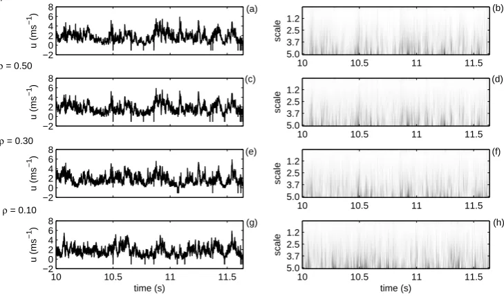
Fig. 3. Surrogate time series for theu1dataset from Fig. 1 are shown in the left hand column for stated values ofρ, while the right hand
column gives the corresponding absolute part of the continuous wavelet transform for each surrogate series using a Mexican Hat wavelet applied to the first 5 scales (formed using 81 voices). Differences would be less visible if more scales had been displayed because the higher
energy at higherjmeans that a greater proportion of coefficients are fixed.
where the H¨older/lipshitz exponents,α fall within the sup-port of the multifractal spectrumD(α). Figure 3 shows that asρincreases, the time series converges upon that in Fig. 1a. In addition, it illustrates how the resulting wavelet modulus maxima are preserved. For example, note that at scale≈5 andt≈10.9 s an energetic feature is fixed forρ≥0.3, but the feature at scale≈5 andt≈11.25 s is only fixed forρ≥0.5.
For the replication of the wavelet transform modulus max-ima it is necessary for the surrogates to preserve the mul-tifractal spectrum of the original data, and that this is only accomplished over all scales at high values forρ. However, it is also the case that there is both an imprecision in the cal-culation of theαexponents due to the limitations of the reso-lution and length of the datasets, as well as imprecision in the signal itself owing to instrument noise etc. Hence, at a some-what lower value forρthere will be no significant difference between surrogates and a multifractal dataset, depending on the width of the support of the multifractal spectrum. This issue is examined in Sects. 6.3 and 7.
3.4 Evaluating finite size effects on randomisation
Clearly, in the limit ofρ=1 the surrogates and dataset are identical and no randomisation occurs. Hence, the issue of finite size effects is complex as it will be a function of the length and nature of the time series, and the chosen value forρ. For example, the highest value (ρ = 0.999) used in this paper leaves, on average (calculated over 200 surrogates)
447 values in the same positions in Fig. 1 as they are in the surrogate (≈5% of N=8192). For a very short seg-ment of this time series of 256 velocity values and averaged over 500 surrogates, forρ∈ {0.5,0.9,0.99}, 2.7 (1%), 15.5 (6%) and 49.4 (19%) of values were fixed in place. These values may be compared to similar results for a time series also of 256 points, but of a very different structure - the sunspot data analysed in Keylock (2007). In that case, for
ρ∈ {0.5,0.9,0.99}, on average 2.8 (1%), 13.4 (5%) and 37.5 (15%) of values were fixed in place. Hence, finite size ef-fects need to be considered for very high values forρwhen datasets are short because a perceived increase inρ will not have altered the nature of the time series. However, the exam-ple applications of the technique in this paper retain sufficient degrees of freedom for sufficient randomisation to occur.
0 200 400 600 800 1000 0
200
time 0
200 0 200 0 200
0 200 0 200
(a)
(b)
(c)
(d)
(e)
(f)
ρ = 1.00
ρ = 0.00
ρ = 0.20
ρ = 0.70
ρ = 0.50
ρ = 0.97
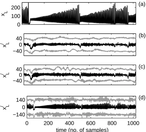
Fig. 4. Example realisations of the Santa Fe laser intensity data,xL,
for various choices ofρ. Figure 4a is the original data series. The
other 5 time series are those for the surrogate with the median value
forAλs=1at the appropriate value forρin Fig. 5. The values forρ
are 0.00 (3b); 0.20 (3c); 0.50 (3d); 0.70 (3e); 0.97 (3f).
4 An application to the time asymmetry behaviour of a laser intensity time series
Figure 4a shows 1024 values from the Santa Fe laser time series,xL, (Huebner et al., 1989). This is a well-known test
data series in nonlinear science. Example surrogate series for different choices ofρare given in Fig. 4b–f. The surro-gates shown in Fig. 4 are those corresponding to the median value for the surrogate asymmetry in Fig. 5. While visually, a choice ofρ≈0.5 qualitatively begins to resemble the orig-inal data, gradual wavelet reconstruction is used to study the behaviour of these data using the temporal asymmetry (or skewness) measureA(Schreiber and Schmitz, 1997):
Aλ=D(xt−xt−λ)3
E
/D(xt−xt−λ)2
E32
(5) where the standard choice in testing for nonlinearity is to chooseλ=1 (Schreiber and Schmitz, 1997). There is a logic for choosingλ=1 for this dataset because the autocorrela-tion funcautocorrela-tion has crossed zero byλ=2, going from 0.53 at
λ=1 to−0.19 atλ=2. Adopting an ensemble of different choices forλ gives additional information on the nature of the nonlinearity within the dataset and provides further crite-ria that one could aim to replicate when attempting to model a time series.
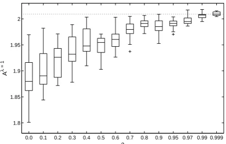
Figure 5 gives values for Aλ=1 for 19 surrogates, at 14 choices forρ, as well as the value for the laser data,AλL=1, which is indicated by a dotted line. From Fig. 5, the null hy-pothesis is rejected untilρ=0.97. Hence, although there are visual similarities between Fig. 4d and the original intensity data, a much higher choice forρis required to preserve the key elements of the signal with respect to asymmetry.
0.0 0.1 0.2 0.3 0.4 0.5 0.6 0.7 0.8 0.9 0.95 0.97 0.99 0.999 1.8
1.85 1.9 1.95 2
A
λ
= 1
ρ
Fig. 5. Gradual wavelet reconstruction of the laser intensity data
based on the one step time asymmetry,Aλ=1. The dotted line gives
the value forAλL=1. The boxplots are the values for the 19
surro-gates, where the box indicates the upper and lower quartiles, the central line is the median and the whiskers extend up to 1.5 times the interquartile range, with outliers indicated by a +. Note the non-linear scale on the abscissa.
Figure 6 shows the original Santa Fe laser series,xL, for
reference (Fig. 6a) together with the difference,xL/, between
xLand surrogate data series (in grey and displaced vertically
by±40 (Fig. 6b and c) or±140 (Fig. 6d), as well as a series defined by the fixed wavelet coefficients (i.e. with no stochas-tic, unfixed coefficients added), which is shown in black, for the three choices ofρ. In every case, the surrogate series for
xL/ that is displaced downwards is that with the median value forAλ=1in Fig. 5, and that displaced upwards is the series with the maximum. The key difference between the series whose value forAλ=1exceeds that forAλL=1(the upper grey line in Fig. 6b) and all the other data shown (including the fixed part of the data series forρ=0.97) is that the unfixed coefficients have acted to remove the discontinuity that oc-curs after 70 samples, where there is a sudden transition in the behaviour ofxL. Hence, it would appear that, in addition
to the general saw-tooth nature of the laser intensity, repre-senting this type of discontinuity correctly is essential if a model for this system is to replicate the asymmetry charac-teristics of the original data.
StudyingAλ=4andAλ=6, which are the lags greater than zero with the minimum and maximum autocorrelations (R= −0.62 and R=0.75, respectively), one finds that the null hypothesis is rejected untilρ=0.97 and untilρ=0.999, re-spectively. Thus, more rigorous model validation can be ac-complished by deploying additional choices for λ. Going further, an ensemble of different metrics could also be em-ployed, a topic that is considered in Sect. 6.
0 100 200
x L
−40 0 40
x L
/
−40
0 40
x L
/
0 200 400 600 800 1000
−140 0 140
time (no. of samples)
x L
/
(a)
(b)
(c)
(d)
Fig. 6.xLis shown in (a), while (b–d) illustrate the difference (in-dicated by a prime) between this time series and various surrogates
series at 3 choices forρ (0.97 in 6b, 0.95 in 6c, and 0.50 in 6d).
The black line in these cases representsxL−xF, wherexF is a data
series produced solely from the fixed wavelet coefficients. The grey
lines showxLxswhere the upper surrogate series maximizesAλs=1
at thisρ in Fig. 5, and the lower series has the median value for
Aλs=1.
˙
y1=σ (y2−y1) ˙
y2= −y1y3+R y1−y2 (6)
˙
y3=y1y2−by3
and one on a set of five ordinary differential equations that constitute a complex-valued Lorenz model due to Zeghlache and Mandel (1985):
˙
y1= −σ (y1+δ y2−y3) ˙
y2= −σ (y2−δ y1−y4) ˙
y3= −y3+R y1+δ y4−y1y5 (7)
˙
y4= −y4+R y2−δ y3−y2y5 ˙
y5= −by5+y1y3+y2y4
whereb, the Rayleigh number,R, and the Prandtl number,
σ, are the three classic parameters of the Lorenz model and
δ represents the detuning between the frequencies for the electric field and the atomic polarization in this application. Hence, whenδ=0 andy2=y4=0 we recover the standard Lorenz model.
Huebner et al. (1989) found that these two models gave a reasonable fit to the original data in terms of their value for
0 100 200 300 400 500 600 700 800 900 1000 0
200 400
xL
(Lorenz)
0 100 200 300 400 500 600 700 800 900 1000 0
100 200 300 400
xL
(complex Lorenz)
time (no. of samples)
(b) (a)
Fig. 7. Output from the two models for the laser series, formed
by squaring they1 output from Eqs. (6) and (7), which may be
compared to the series,xL, in Fig. 4a and a surrogate withρ=0.97
in Fig. 4f.
the correlation dimension measure adopted in Sect. 5, imply-ing that Lorenz-type models are suitable for modellimply-ing such time-series. To test this hypothesis with respect to our skew-ness/asymmetry measure, we integrated both sets of equa-tions using a time step of 0.01 and choosing the values:
b=0.25, R=15, σ=2, and δ=0.05, as per Huebner et al. (1989). In both cases, the time series fory12 was down-sampled such that the time to the first zero crossing of the autocorrelation function matched that in the original dataset (2 samples) andAλ=1was calculated for series of 1024 val-ues. We obtainedAλ=1=2.207 for the Lorenz model and
Aλ=1=2.624 for the complex Lorenz model. These results are higher than the value for the laser data ofAλ=1=2.008, but it is not immediately clear if this difference is significant. Using the results in Fig. 5 we see that atρ=0.97 there is no significant difference between the original data and the surrogates forAλ=1. Both asymmetry values for the mod-els are much greater than the largest value ofAλ=1=2.017 found for the 19 surrogates at this choice ofρ. Going fur-ther, 200 surrogates were generated forρ=0.97 and a Ryan-Joiner test for normality showed theAλ=1values to be nor-mal at the 10% significance level. Based on the standard de-viation of 0.0078, the asymmetry values for the models are 79 and 25 standard deviations from the value for the data. Hence, the probability of obtaining the models’ asymmetry values based on surrogates at a value forρ with the greatest intrinsic variability that preserve the asymmetry properties, is vanishingly small. The difference in the nature of the model signals is illustrated in Fig. 7. For the additional choices of
5 An application to the Lorenz system
The Lorenz equations are the paradigmatic chaotic system, although it is only relatively recently that a comprehensive study of all three parameters of this model has been under-taken (Barrio and Serrano, 2007, 2009). In this section of the paper we employ classical choices forb=8/3 andσ=10, but consider values for the Rayleigh number,R, that include the classical, globally attracting chaotic attractor (R=28), a value (R=24.29) that gives a chaotic attractor with a pair of stable attracting rest points, a value ofR=24.75 by which the stable points have been eliminated (see Kaplan and Yorke, 1979), and a value within the regime of an intermit-tent transition to chaos identified by Manneville and Pomeau (1979) and Pomeau and Manneville (1980) (R=167.0).
The Lorenz equations were solved with a time step of
t=0.01, with results recorded every tenth time step fromt=
1000. The accuracy of our numerical method was checked by using the Gottwald and Melbourne (2005) test for chaos ap-plied toy1. The transition to chaos atR=166.0616 found using this method was in agreement with the value found us-ing the methods of Barrio and Serrano (2007) (personal com-munication from Roberto Barrio).
In this study we employed the correlation dimension,Dc,
as a means of characterising the attractor (Grassberger and Procaccia, 1983) based on a Gaussian kernel method and using the output fory1, with lags and Theiler windows de-fined based on the decay of the autocorrelation function and on false nearest neighbours, respectively. We tested our method for long (40 960 points) and short (4096 points) datasets. Grassberger and Procaccia (1983) quote a value of
Dc=2.05±0.01 for the correlation dimension at R=28,
which was matched successfully by both of our datasets (Dc=2.052 andDc=2.055, for long and short datasets,
re-spectively). Hence, we employed the shorter series in analy-sis. It is possible to obtain erroneous, finite correlation di-mensions for stochastic processes (Schertzer et al., 2002). However, by working with a system that is known to ex-hibit chaos and by deploying high values forρ that ensure the basic structure of the Lorenz attractor is fixed in place (much as it would be for data from a Lorenz attractor with noise),means that we have generated correlation dimensions for data that are approximating the original, chaotic attrac-tors.
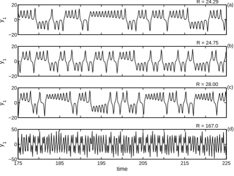
Figure 8 illustrates short time series for y1 for the four choices ofR examined here. Figure 9 gives the correlation dimension as a function of embedding dimension,De, for our
four choices ofR. The embedding dimension is the dimen-sion of the phase space into which the time series is embed-ded based on delayed versions of the original series (Takens, 1981). An accurate estimate forDcrequiresDeto be
suffi-cienly large to capture the dimension of the attractor (i.e. at least 3 for the Lorenz system) but not so great as to intro-duce errors from finite size effects. For a time series,y1it is possible to form a set ofN−(De−1)Lvectors:
175 185 195 205 215 225
−50 0 50
time
y1 −20
0 20
y1
−20 0 20
y1
−20 0 20
y1
(a)
(d) (c) (b)
R = 28.00
R = 167.0 R = 24.75 R = 24.29
Fig. 8. Subsections for time series from the Lorenz equations for
different choices ofR.
Yi=(yi,yi+L,...,yi+(De−1)L) (8)
each of which defines a point in this embedding space, where
Lis a lag andN is the number of values in the time series. Gradual wavelet reconstructions based on 19 surrogates are shown for two choices ofρ, 99% (blue error bars) and 99.9% (red error bars). In addition, reconstructions at these values forρare shown based purely on the fixed wavelet co-efficients without using the IAAFT algorithm to re-introduce the unfixed coefficients (as described at the end of Sect. 3.1). These are indicated by the dotted lines, with the circles show-ingρ=0.99 and the squaresρ=0.999. The error bars are displaced a small horizontal distance from the integer value forDeand indicate the mean and±2 standard deviations by
horizontal lines.
The most similar plots are Fig. 9b and c, both of which are within the same regime of behaviour forRaccording to Kaplan and Yorke (1979). In these cases, at ρ=0.99 the dataset built from just the fixed coefficients clearly differs from the original data. The surrogate data (blue error bars) are generally even further from the original data on average, but within the ±2 standard deviation tolerance of both the original data and the fixed coefficient surrogate (particularly whenR=28.00). The higher choice forρresults in a conver-gence of both types of surrogate to the original data. Thus, at
ρ=0.99, on average for these two cases, the addition of the unfixedwj,kto the surrogates results in greater error than a
lack of precise preservation of the data histogram or wavelet spectrum from just using the fixed coefficients. However, by
ρ=0.999 this other error source is dominant and realisations built from just the fixed coefficients contain greater error. A more in-depth analysis could examine the precise values for
1.5 2 2.5 3 3.5
D c
0 5 10 15
1.5 2 2.5 3 3.5
D
e
D c
0 5 10 15
D
e
(d) (b)
(c) (a)
Fig. 9. The correlation dimension,Dc, as a function of embedding dimension,De, for the Lorenz system and surrogates withR=24.29
(a),R=24.75 (b),R=28.00 (c), andR=167.0 (d). The results for the Lorenz system are given by a black line, with those for series
reconstructed from the fixed wavelet coefficients forρ=0.99 (dotted line with circles) andρ=0.999 (dotted line with squares) and surrogate
series forρ=0.99 (blue) andρ=0.999 (red). The latter summarise results for 19 surrogates according to mean (central horizontal line) and
±2 standard deviations (vertical lines). They are translated slightly from the integer value forDefor clarity.
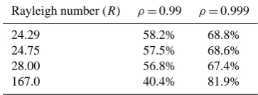
Table 1. The proportion of wavelet coefficients fixed in place as a
function ofRfor our two choices ofρ.
Rayleigh number (R) ρ=0.99 ρ=0.999
24.29 58.2% 68.8%
24.75 57.5% 68.6%
28.00 56.8% 67.4%
167.0 40.4% 81.9%
The situation differs in Fig. 9a, where the error bars for the gradual wavelet reconstruction are all small and lie close to the original data. However, forρ=0.99 there is a clear difference for the surrogate built purely from the fixed coef-ficients, which sits outside the error bars for the surrogates. In this case, failure to preserve the wavelet spectrum and his-togram accurately has had a significant effect onDc, while
randomisation by the unfixed coefficients has a minimal ef-fect.
The situation differs again in Fig. 9d, where this time at
ρ=0.99 it is the realisation from the fixed coefficients that lies significantly closer to the original data than the surro-gates. Hence, the randomised coefficients generate greater error than the failure to preserve the histogram or spectrum. For this case, it is also notable that byρ=0.999, while both
types of surrogates have converged upon one another, none have converged on the original data. Table 1 lists the propor-tion of coefficients fixed at the two chosen thresholds. For
ρ=0.99 andR=167.0 there is a small proportion of fixed coefficients (i.e. there is high energy in relatively few val-ues). This means that the randomisation within the surro-gates is causing a relatively weak convergence on the scal-ing behaviour ofDc. However, byρ=0.999 more
coeffi-cients are preserved for this dataset than the others yet the surrogates still differ significantly (at the 10% level) from the original data. This shows that the attractor for the Pomeau and Manneville intermittency regime is more complex than for the other values for R used here in the sense that, the value forDc in the data can only be replicated by fixing in
10−2 10−1 100
10−4
10−2
100
102
frequency (rad−1)
Power
spectral density
Dau8 O5 O5L O5P O6 O7 O8 O9 O10 O10L O10P O12
0 0.5 1
α
(t)
0 0.1 0.2 0.3 0.4 0.5 0.6 0.7 0.8 0.9 1
0 0.5 1
time
α
(t)
(a)
(b)
(c)
Estimation method
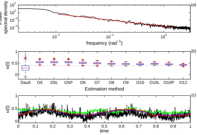
Fig. 10. Testing the oscillation-based method and a wavelet-based algorithm for estimating H¨older exponents. (a) Shows the spectrum of
a fractional Brownian motion and a fitted slope, which is translated into a value forαin (b) (dotted line). The box and whisker plots in
(b) show the median, upper and lower quartiles (boxes) values extending up to 1.5 times the interquartile range (whiskers) and outliers (red
crosses) for the set of 4096 estimated values forα(t )as a function of the algorithm used. A wavelet method using a Daubechies wavelet
with 8 vanishing moments is indicated by Dau8, while “O” indicates the oscillation method. The number following the “O” is the largest
exponent used in the calculation forδ. Hence, “O8” means that the bins forδranged from 21to 28. Least-squares regression was used unless
a suffix “L” (Lim Inf regression) or “P” (penalised least-squares regression) is included. See (FRACLAB, 2006) for more details. (c) Shows
the sinusoidal function forα(t )used to generate a multifractional Brownian motion (blue line) and then estimated values forα(t )from that
multifractional Brownian motion time series. The black line is the Dau8 algorithm, the green line is O5 and the red line is O10.
6 The H¨older characteristics of a turbulence time series
There have been a number of studies that have tried to char-acterise the multifractal characteristics of turbulence (e.g., Meneveau and Sreenivasan, 1987; She and Leveque, 1994) owing to the well-known intermittency characteristics (e.g., Frisch et al., 1978) that lead to a departure from Kol-mogorov’s 13 scaling as discussed by Kolmogorov (1962). However, the predictions of the latter’s log-normal model differ from the log-Poisson model of She and Leveque (1994) and analyses based on universal multifractal scaling (Schertzer and Lovejoy, 1992; Schmitt et al., 1992) provide an alternative framework for classifiying these processes.
It has recently been proposed to make use of the point-wise roughness characteristics of a turbulence velocity time series, u(t ), to isolate the periods of high activity in en-vironmental turbulence data (Keylock, 2008b, 2009) using H¨older/Lipshitz exponents,αu(t ). That is, the
differentiabil-ity of a signal relative to polynomial approximations within the local domain of a specific point are used to deriveαu(t ).
Hence, studyingu(t ) in a neighbourhood, δ, about a posi-tion,T, and takingtandT to be rescaled over the unit inter-val (ranging from 0.0 to 1.0), we obtain from a Taylor series expansion:
pT(t )= m−1
X
i=0 u(i)(T )
i! (t−T )
i (9)
wheremis the number of times that u is differentiable in
T±δ. Defining the error in approximatingu(t )atT bypT(t )
as
T(t )=u(t )−pT(t ) (10)
means that the order of differentiability of u(t )close toT
gives an upper bound onT(t ):
|T(t )| ≤
|t−T|m
m! (11)
This upper bound is then given by a non-integer H¨older/Lipshitz exponent, where a functionu(t )has a point-wise H¨older exponent, αu≥0 if a constant K >0 and the
polynomialpT(t )of degreemexists such that
|u(t )−pT(t )| ≤K|t−T|β (12)
The H¨older regularity,αu(t ), ofu(t )atT is then given by the
−0.1 0 0.1
R(u
1
u 2
)
0 0.02 0.04
γ
* (u S
1
u 2
)
0 0.25 0.5
R(
α u 1
u 2
)
0 0.25 0.5
γ
* (α S
u 1
u 2
)
0 0.1 0.2 0.3 0.4 0.5 0.6 0.7 0.8 0.9 0.95 0.97 0.99 0.999
0.04 0.05 0.06 σ av
(a)
(b)
(c)
(d)
(e)
ρ
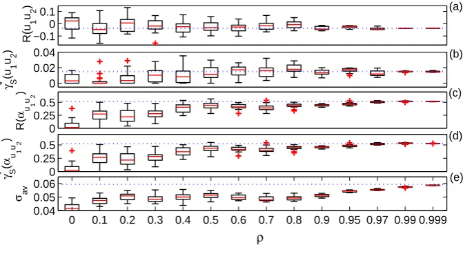
Fig. 11. Gradual wavelet reconstruction for the H¨older series of the two components of the velocity data from Fig. 1. The measures used are
the correlation between the velocity series (a) and H¨older series (c), the phase synchronisation between the velocity series (b) and the H¨older series (d), and the average standard deviation of the H¨older series (e).
6.1 Calculating H¨older exponents
A rapid method for evaluating αu(t )is based on a log-log
regression of the signal oscillations,OT±δ, within some
dis-tanceδofT againstδ, whereOT±δis given by:
OT±δ=max(ut∈(T−δ,...,T+δ))−min(ut∈(T−δ,...,T+δ)) (13)
andδ is distributed logarithmically (from 21 to 210 in this study).
This approach was discussed by Kolwankar and L´evy Ve-hel (2002) and considered to be more accurate than wavelet based methods. For the comparison of the differential sensi-tivity of metrics to the presence of multifractality (Sect. 6.2), using correlation, non-linear association by phase synchro-nisation, and on the variance of the estimatedαu(t ), as
de-scribed below), we require a precise and consistent estimator for the H¨older regularity.
Figure 10 evaluates different methods for calculating H¨older exponents and supports the use of the oscillation-based method. Figure 10a shows the power spectral den-sity for a fractional Brownian motion (N=4096) and the fitted slope (red line) from this plot is shown as a H¨older exponent in Fig. 10b with a black dotted line. The DWT (see Appendix A) wavelet-based method using a Daubechies wavelet with 8 vanishing moments is clearly the least precise method. The accuracy and precision of the oscillation-based method increases as the size of the bins used to estimateδ
increases. The results are much more sensitive to this than the particular method used to fit the log-log regression line. Figure 10c shows a sinusoidal curve in blue that was used to prescribe the variation ofα(t )for a multifractional Brown-ian motion. This signal itself is not shown but attempts to back-estimate the α(t )from this signal are given in black
(DWT-based method), green (least-squares oscillation-based method with the bins forδ ranging from 21to 25- O5) and red (least-squares oscillation-based method with the bins for
δranging from 21to 210- O10). Our choice of the O10 algo-rithm is the most precise. These calculations were performed using the FRACLAB toolbox (FRACLAB, 2006).
6.2 The differential sensitivity of particular metrics to the presence of multifractality
For a choice ofρ=0, the surrogate series will preserve the Fourier spectrum to some error level, but not the intermit-tency (multifractal characteristics). Asρ→1, the variance of the H¨older series tends towards that for the original data. Our gradual wavelet reconstruction of the turbulence data in Fig. 1 is based on 19 surrogates and compares the sensitivity of five metrics to the presence of (multifractal) nonlineari-ties: correlations between the velocity series,R(u1u2), and H¨older series,R(αu1u2), the phase synchronisation between
these respective series,γS∗(u1u2), andγS∗(αu1u2), and the
av-erage standard deviation of the H¨older series across the two components:
σav= [σ (αu1)+σ (αu2)]/2 (14)
Phase synchronisation is a nonlinear method of association between data series and the procedure we adopted for its cal-culation is given in Appendix B.
0 0.05
|w
1,k
|
−0.020
0.02
|w
1,k
/
|
−0.010
0.01
|w
1,k
/
|
0 0.1 0.2
|w
4,k
|
−0.0020.000
0.002
|w
4,k
/
|
10.900 10.925 10.950 10.975 11.000 11.025 11.050 11.075 11.100
−0.0010.000
0.001
|w
4,k
/
|
time (s)
(a)
(b)
(c)
(d)
(e)
(f)
Fig. 12. Modulus maxima of wavelet coefficients for the time series foru1are shown in (a) and (d) atj=1 andj=4, respectively. The data
in (b) and (c), as well as (e) and (f) show the difference (indicated by a prime) between|wj,k|and the values from a wavelet decomposition
of a surrogate data series (forρ=0.99 in (b) and (e), and shown in red; forρ=0.999 in (c) and (f), and shown in blue).
−0.04 −0.02 0 0.02 0.04
benzi (
σmedian
)
0 500 1000 1500 2000 2500 3000 3500 4000 −0.04
−0.02 0 0.02 0.04
time
benzi (
σmax
)
(a)
(b)
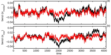
Fig. 13. Two realisations of the Benzi et al. (1993) process are given
in black, with their stationary variants in red. From the 50 datasets generated, the data in (a) had the median value for the standard
deviation ofα(t )and (b) had the maximum.
the multifractal characteristics of the signal. However, when the H¨older series are examined, both of these two measures show significant differences forρ <0.40. The null hypothe-sis is rejected at all our choices forρusing the average stan-dard deviation measure, indicating that this is the most sensi-tive to the multifractal characteristics of the two series. Our technique permits the relative sensitivity of different metrics to be determined empirically for particular data and it is in-teresting here that the sensitivity of the correlation and its nonlinear, phase synchronisation counterpart appears to be approximately the same.
From Fig. 11e it follows that intermittency in the surro-gates has yet to converge on the data at the highest choices for ρ used in this paper. Part of the reason for this is the broad-band nature of the turbulence signal compared to the Lorenz attractor, for example. Table 1 has typical values of
57% and 68% of wavelet coefficients fixed forρ=0.99 and
ρ=0.999, respectively, while the equivalent percentages are 26.1% and 40.1% foru1, and 17.4% and 30.8% foru2. In-creasingρto 0.9999 still only fixes 55.1% and 45.1% of the coefficients, respectively. This is why a sparse, wavelet rep-resentation of a turbulence signal is such an effective descrip-tor (half the coefficients contain 99.99% of the energy).
Figure 12 shows, for two wavelet scales, the modulus max-ima of the wavelet coefficients for the data (black) and the difference between this series and that for surrogates gener-ated atρ=0.99 (red) andρ=0.999 (blue). Note that while the values in Fig. 12d are roughly double those in Fig. 12a, the errors are an order of magnitude lower. Hence, for both choices for ρ there are a number of features at the finest wavelet scales whose energy is too small to be fixed, yet which contribute actively to the singularity structure of the time series, affecting the values for the H¨older series in the surrogates and the value forσavfor these data.
However, it is also the case that:
1. Determining the multifractal properties of a signal is a difficult task (Lux, 2004; Seuret, 2006);
2. The variance measure given by Eq. (14) is more depen-dent on the absolute accuracy of our method for eval-uating H¨older exponents than the other metrics used in Fig. 11; and,
3. Different realisations of a stochastic multifractal pro-cess will lead to intrinsic variability in the estimated values forα(t ).
Data 0.020 0.025 0.030 0.035 0.040
σ
(
α benzi
)
0 0.1 0.2 0.3 0.4 0.5 0.6 0.7 0.8 0.9 0.95 0.97 0.99 0.999
ρ
Fig. 14. Gradual wavelet reconstruction of the dataset giving the median value forσ (αbenzi)based on fifty realisations of the multifractal
process is shown in the right-hand figure. The left-hand figure is a boxplot giving the inherent variability ofσ (αbenzi)for the 50 datasets.
the finite precision of the O10 algorithm. A comparison with another multifractal dataset helps to interpret these results appropriately.
6.3 The standard deviation of H¨older exponents for multifractal data
We employed a wavelet-based algorithm for generating mul-tifractal data due to Benzi et al. (1993). This is a stochas-tic algorithm based on a discrete wavelet transform, whereby wavelet coefficients are assigned and then the inverse wavelet transform is used to construct the time series. Here we follow Benzi et al. (1993) and take an initial, arbitrary coefficient,
χ0,0, representing theJ+1 wavelet scale, and then form the wavelet coefficients at scalesj=J,...,1, hierarchically ac-cording to the recursion:
χj,k=j,kηj,kχj+1,k0 (15)
wherek0=1
2k,j,ktakes the values±1 with equal probabil-ity, and the random variableηj,khere takes the values 2−5/6
or 2−1/2with probabilities of 0.875 and 0.125, respectively. Fifty datasets were generated and two example realisations are shown in black in Fig. 13.
To reduce the variability in the data that would contribute to changes in the variance of the αbenzi values for the 50 datasets, the stationarity of each realisation was improved by setting MODWT approximation and the detail coefficients at
j=J−2,...,J to zero (the red signals in Fig. 13). Thus, variability at scales that are affected by the finite length of the record (212 values) was removed. Furthermore, to elim-inate any problems due to end effects, theα(t )values were calculated over the central 211 values. The degree of vari-ability forσ (αbenzi)for all 50 realisations based on this pro-cedure is given by the left-hand boxplot in Fig. 14. A gradual
wavelet reconstruction for the dataset with the median value forσ (αbenzi)(shown in Fig. 13a) is then undertaken on the right-hand side of Fig. 14.
The first thing to note is that the multifractal properties of the time series are recovered some way before the limit ofρ→1. Hence, the result from Fig. 11e is not generally true for all multifractal datasets. For the Benzi et al. (1993) process, IAAFT surrogates are able to match the values for
σ (αbenzi)and, working from the right, the surrogates become significantly different to the dataset atρ=0.95. Given that we took care to minimise variability in the calculation of
σ (αbenzi) resulting from finite size effects, it is also note-worthy that the variability for the 50 realisations on the left of Fig. 14 is greater than for even the IAAFT surrogates. Hence, the O10 algorithm used here would appear to be suffi-ciently precise both in absolute terms (Fig. 10c) and relative to the intrinsic variation of similarly generated, sotchastic, multifractal time series. Thus, the analysis of the turbulence dataset in Sect. 6 shows that σav is the measure most
sen-sitive to the presence of multifractality, but the observation that even whenρ=0.999 the surrogates differ from the data is not true in general for all multifractal series. I.e. gradual wavelet reconstruction can mimic relevant properties of mul-tifractal data at values forρ <1.
7 The precision of our technique for evaluating H¨older exponents
0 0.05 0.1
σ
(
α x
)
0 0.05 0.1
σ
(
α x
)
0 0.1 0.2 0.3 0.4 0.5 0.6 0.7 0.8 0.9 0.95 0.97 0.99 0.999
0 0.05 0.1 0.15
σ
(
α x
)
ρ
(a)
(b)
(c)
Fig. 15. Gradual wavelet reconstruction of multifractional Brownian motions given by Eq. (16) withf=0.005 (a),f =0.010 (b), and
f=0.015 (c). The metric employed is the standard deviation of the calculated H¨older exponents.
αx(t )=0.33+fsin(4π t ) (16)
wheret ranges from 0 to 1 and containsN=2048 values, and the amplitude,f∈ {0.005,0.01,0.015}. Hence, the mean value forαuequates to that for inertial range turbulence. As f →0 we should reach a value where imprecision in our algorithm means that we cannot discriminate between a truly (but weak) multifractional Brownian motion and a fractional Brownian motion with a Hurst exponent of 0.33. That is, the values for the metric applied to the IAAFT surrogates do not differ significantly than that for the data.
The H¨older characteristics of the derived time series and their surrogates were evaluated using the O10 method. From Fig. 15, it is clear that asf increases,σ (αx)for the data
(the dotted blue lines) also increases, as expected. Moving leftwards from the right-hand side of these plots a significant difference emerges in Fig. 15a atρ=0.95, while it occurs at
ρ=0.97 in Fig. 15b and c. Both of these values are lower than seen in Fig. 11e, while the results in Fig. 15a are very similar to those in Fig. 14. The variability whenρ=0 is rela-tively constant for varyingf, meaning that, becauseσ (αx)is
lower in Fig. 15a, there is no significant difference between the observed value and those for IAAFT surrogates when
f=0.005. The complex nature of Fig. 15a (and Fig. 14) shows that no significant difference occurs when the surro-gates are unconstrained, owing to the relatively large inher-ent variation in the time-series and the relatively weak ex-pression of the multifractality. However, as ρ∼0.9, suffi-cient energy has been fixed in place for the surrogates to be a trained upon the original data, but with such random variabil-ity thatσ (αx)is too low. It is only byρ=0.97 that sufficient
energy is fixed for no significant difference to occur again. In contrast, the degree of multifractality in Fig. 15b and c is sufficient for the gradual wavelet reconstructions to be more
simply structured, meaning that the precision of our O10 al-gorithm is sufficient to detect variability in H¨older exponents at a value for 0.005< f <0.01 and above.
8 Conclusions
This paper has presented a methodology for exploring prop-erties of nonlinear time series through the systematic vary-ing of an energy threshold and the construction of surro-gate datasets that conform to this threshold using a wavelet transform. For a given threshold, either one realisation can be obtained based on the wavelet coefficients fixed at that threshold, or the unfixed coefficients can be added back to the wavelet template in an appropriately constrained, stochastic fashion using the IAAFT algorithm to give multiple realisa-tions. Comparing the value of a metric with the values for the wavelet reconstructed series at multiple choices forρpermits certain properties of the signal or the metrics to be elucidated including:
1. the parts of the signal that need to be preserved to give a value for the metric similar to the original data (laser data example in Sect. 4);
2. assessing how closely model results match the value for the metric for the data (Sect. 4);
3. classification of time series complexity (Lorenz equa-tions example in Sect. 5);
4. the sensitivity of different metrics (turbulence example in Sect. 6); and,
With regards to the multifractal characteristics of geophysi-cal data, an alternative perspective on the methodology pre-sented here would be to re-define the analysis such that the starting point is not a linear variant of the original signal, but a multifractal variant of the original signal. Recently, Palus (2008) has proposed a pertinent multifractal surrogate gener-ation algorithm. This development would see the work pre-sented herein take a new direction. In this paper, departures from monofractality of increasing strength will correspond to increases in the value forρat which significant departures are first detected (Sect. 7). Imposing the multifractal struc-ture at the start would be potentially of interest if one wished to see how a metric that was not directly related to the multi-fractality of the signal (e.g. Eq. 5) was conserved by the sur-rogates as a version ofρ increased but with the multifractal spectrum fixed in addition to the Fourier spectrum and his-togram of values in the data, as is the case in this study. This alternative version of gradual wavelet reconstruction will be explored in the future.
Appendix A
Wavelet transforms
A1 The continuous transform
A continuous wavelet transform (CWT),w(j,k) of a time seriesx(t )at a scale,j >0, and a position,k∈ <, is given by the convolution of the time series with a wavelet function,ψ, whose integral is zero, and whose square integrates to unity:
w(j,k)=√1 j
Z +∞
−∞
x(t )ψ∗(t−k/j )dt (A1)
where∗is the complex conjugate. An additional admissibil-ity constraint on the form of the wavelet function, which per-mits a reconstruction of the original signal, is that its Fourier transform
9(f )≡
Z +∞
−∞
ψ (t )e−2πf t idt (A2)
is such that 0< Cψ<∞, where
Cψ≡
Z ∞
0
|ψ (f )|2
f df (A3)
As such, it follows that Z +∞
−∞
x2(t )dt= 1 Cψ
Z ∞
0
Z +∞
−∞
w2(j,k)dt
dj
j2 (A4)
which shows thatw2(j,k)/j2 is the energy function of the signal decomposed over different scales and positions. This is important in this study as the key parameter,ρ, may be defined in terms of the square of the wavelet coefficients.
A2 The discrete transform
As shown for the IAAFT method in Sect. 2, surrogate data algorithms involve a deconstruction of an original signal, a manipulation and a subsequent reconstruction. The integral in Eq. (A1) makes reconstruction using the continuous trans-form problematic. The discrete wavelet transtrans-form (DWT) is based on a hierarchical set of filtering operations that can be readily used in signal reconstruction. Hence, the DWT has been used in the past for generating surrogate data se-ries (Breakspear et al., 2003). While we prefer an alterna-tive approach, the essence of the DWT is briefly explained to provide relevant context for our favoured transform. Results using a DWT method are also given in Fig. 10b.
A DWT of a time series sampled at N=2J points can
be formulated over the dyadic scales 2j,j=1,...,J using
a filter bank of low and high pass quadrature mirror filters of even filter width,L, wherehl(l=0,...,L−1)is the high
pass (or wavelet) filter,gl is the low pass (or scaling) filter
and
gl≡(−1)l+1hL−1−l (A5)
At the first stage of the algorithm, j=J, these filters are circularly convolved withx(t )and then downsampled by a factor of 2 to give a set of wavelet,w, and approximation,A, coefficients of lengthN/2:
w1,k≡
√
2w˜1,2k+1 k=0,..., N
2 −1
√
2w˜1,k≡ L−1 X
l=0
hlxt−lmodN k=0,...,N−1 (A6)
A1,k≡
√
2A˜1,2k+1 k=0,..., N
2 −1
√
2A˜1,k≡ L−1 X
l=0
glxt−lmodN k=0,...,N−1 (A7)
At subsequent stages of the algorithm,j, the approximation from the previous stage of the algorithm,Aj−1,k is used
in-stead ofxtin Eqs. (A6) and (A7) to give wavelet coefficients
over all scalesj=1,...,J and a final approximation coeffi-cient.
A3 The maximal overlap discrete transform
While the discrete transform gives a compact representation of the signal, it suffers from certain analytical limitations (Percival and Walden, 2000), which are important in the con-text of surrogate generation:
– Because the wavelet filters are not zero phase, align-ing the coefficients with the original time series is not straightforward;
– Circularly shifting x(t ), taking the discrete transform and determining the wavelet power spectrum does not necessarily return the same spectrum as forx(t ). Of these points, it is the last that is the most important from our perspective. Approximate preservation of linear features of the original data, such as the power spectrum is an es-sential part of an algorithm for generating surrogates for analysing nonlinear time series. However, the first point is also relevant as it is desirable that the evaluation of the local energy content of the signal has a certain universality and is not altered by a circular rotation of the original dataset.
The translation invariant, stationary, or Maximal Overlap Discrete Wavelet Transform (MODWT) avoids the above dif-ficulties. It is an undecimated variant of the discrete trans-form, which means that the downsampling undertaken in the DWT is eliminated. This is a disadvantage if one wishes to produce a compact representation of the signal, but has the advantage for analysis of producingN wavelet coefficients at each scale, similar to the CWT in Eq. (A1).
Effectively, a discrete transform is undertaken for allN
circular rotations ofx(t ). For any given minimum rotation ofx(t )most coefficients will be identical to those at the pre-vious iteration meaning that the computation of the MODWT isO(Nlog2N )and notO(N2)(Liang and Parks, 1996).
Defining the filter width at scalej asLj≡(2j−1)(L−
1)+1 and expressing thejth level MODWT high and low pass filters as
˜
hj,l≡hj,l/2j/2
˜
gj,l≡gj,l/2j/2 (A8)
It is clear from Eq. (A5) that the MODWT filters are re-lated to those used in the DWT except for a rescaling to ac-count for the lack of downsampling. Hence, the MODWT wavelet and approximation coefficients are given as (Perci-val and Walden, 2000):
wj,k≡ Li−1
X
l=0 ˜
hj,lxk−lmodN
Aj,k≡ Li−1
X
l=0 ˜
gj,lxk−lmodN (A9)
which may also be compared to the equivalent expressions for the DWT in Eqs. (A6) and (A7). Practical implementa-tion of the MODWT first requires periodizaimplementa-tion of the filters so that, instead of undertaking an explicit circular convolu-tion with Eq. (A8), we perform implicit circular filtering us-ing a standard convolution and a periodized filter, where
˜ h◦j,l≡
+∞ X
n=−∞
˜
hj,l+nN (A10)
Re-expressing Eq. (A9) in terms of Eq. (A10) gives
w◦j,k≡
N−1 X
l=0 ˜
h◦j,lxk−lmodN
A◦j,k≡
N−1 X
l=0 ˜
g◦j,lxk−lmodN (A11)
We may then evaluate Eq. (A11) from a recursion which states that, given the approximation A◦j,k, we may obtain
w◦j+1,kandA◦j+1,kfrom
w◦j+1,k=
L−1 X
l=0 ˜ h◦lA◦
j,k−2jlmodN
A◦j+1,k=
L−1 X
l=0 ˜ gl◦A◦
j,k−2jlmodN (A12)
Percival and Walden (2000) prove that within a MODWT decomposition framework, the discrete variant of Eq. (A4) holds true.
Appendix B
Phase synchronisation measure
The method for evaluating phase synchronisation in this pa-per follows Kreuz et al. (2007) based on a Hilbert transform approach. Defining the analytic signal of a time seriesx(t )
as
x(t )+ix(t )ˆ =ax(t )eiφx(t ) (B1)
wherex(t )ˆ is the Hilbert transform ofx(t ):
ˆ x(t )= 1
πp.v.
Z +∞
−∞
x(t )/t˘ − ˘t dt˘ (B2)
here p.v. is the Cauchy principal value. From Eq. (B1) it then follows that the phase is given by
φx(t )=tan−1
ˆ x(t )
x(t ) (B3)
and given the phases for time seriesx(t )andy(t ), the phase difference is
1φ (t )=φx(t )−φy(t ) (B4)
and the mean phase coherence can be obtained from1φ (t )
by averaging the angular distribution of phases on the unit circle in the complex plane:
γ=
1
N N
X
j=1 ei1φ (t )
(B5)
account for this, phase-shuffled data can be constructed from one of the time series before the phase differences are cal-culated. The mean value of γ for some finite number of phase-shuffled realisations (usually∼10, which is the case in this paper),γ¯S, can then be used to normalise the value of γcalculated from the data according to
γS∗=
0 ifγ <γ¯
S γ− ¯γS
1− ¯γS ifγ≥ ¯γS
(B6)
Acknowledgements. The author is grateful to K. Nishimura, M. Nemoto and Y. Ito for assistance with the wind tunnel experiment that provided the turbulence data for this paper. This work was supported by NERC grant NE/F00415X/1 and the assistance of two referees and the editor in preparing this manuscript is also gratefully acknowledged.
Edited by: D. Schertzer
Reviewed by: three anonymous referees
References
Bacry, E., Muzy, J. F., and Arn´eodo, A.: Singularity spectrum of fractal signals: exact results, J. Stat. Phys. 70, 635–674, 1993. Barrio, R. and Serrano, S.: A three-parametric study of the Lorenz
model, Physica D, 229, 43–51, 2007.
Barrio, R. and Serrano, S.: Bounds for the chaotic region in the Lorenz model, Physica D, 238, 1615–1624, 2009.
Basu, S., Foufoula-Georgiou, E., Lasheremes, B., and Arn´eodo, A.: Estimating intermittency exponent in neutrally stratified atmo-spheric surface layer flows: A robust framework based on mag-nitude cumulant analysis and surrogate analyses, Phys. Fluids, 19, 115102, doi:10.1063/1.2786001, 2007.
Benzi, R., Biferale, L., Crisanti, A., Paladin, G., Vergassola, M., and Vulpiani, A.: A random process for the construction of mul-tiaffine fields, Physica D, 65, 352–358, 1993.
Borgnat, P. and Flandrin, P.: Stationarization via surrogates, J. Stat. Mech., P01001, doi:10.1088/1742-5468/2009/01/P01001, 2009. Borgnat, P., Flandrin, P., Honeine, P., Richard, C., and Xiao, J.: Testing Stationarity With Surrogates: A Time-Frequency Ap-proach, IEEE Trans. Sig. Proc., 58, 3459–3470, 2010.
Breakspear, M., Brammer, M., and Robinson, P. A.: Construction of multivariate surrogate sets from nonlinear data using the wavelet transform, Physica D, 182, 1–22, 2003.
Daubechies, I.: Orthonormal bases of compactly supported
wavelets: II. variations on a theme, SIAM J. Math. Anal. 24, 499–519, 1993.
FRACLAB: A fractal analysis toolbox for signal and image pro-cessing, http://fraclab.saclay.inria.fr/, 2006.
Frascati, A. and Lanzoni, S.: Long-term river meandering as a part of chaotic dynamics? A contribution from mathematical mod-elling, Earth Surf. Proc. Land., 35, 791–802, 2010.
Frisch, U., Sulem, P. L., and Nelkin, M.: Simple dynamical model of intermittent fully developed turbulence, J. Fluid Mech., 87, 719–736, 1978.
Fritsch, F. N. and Carlson, R. E.: Monotone Piecewise Cubic Inter-polation, SIAM J. Numerical Analysis, 17, 238–246, 1980. Gagnon, J. S., Lovejoy, S., and Schertzer, D.: Multifractal surfaces
and terrestrial topography, Europhys. Lett., 62, 801–807, 2003.
Gottwald, G. A. and Melbourne, I.: Testing for chaos in determin-istic systems with noise, Physica D, 212, 100–110, 2005. Grassberger, P. and Procaccia, I.: Characterization of strange
attrac-tors, Phys. Rev. Lett., 50, 346–349, 1983.
Huebner, U., Abraham, N. B., and Weiss, C. O.: Dimensions and entropies of chaotic intensity pulsations in a single-mode far-infrared NH3 laser, Phys. Rev. A, 40, 6354–6365, 1989. Jaffard, S.: Multifractal formalism for functions: Parts I and II,
SIAM J. Numerical Anal. 28, 944–998, 1997.
Johnson, J. R. and Wing, S. A.: Solar cycle dependence of non-linearity in magnetospheric activity, J. Geophys. Res., 110, A04211, doi:10.1029/2004JA010638, 2005.
Kaplan, J. L. and Yorke, J. A.: Preturbulence: A regime observed in a fluid flow model of Lorenz, Commun. Math. Phys., 67, 93–108, 1979.
Keylock, C. J.: Constrained surrogate time series with preservation of the mean and variance structure, Phys. Rev. E, 73, 036707, doi:10.1103/PhysRevE.73.036707, 2006.
Keylock, C. J.: A wavelet-based method for surrogate data genera-tion, Physica D, 225, 219–228, 2007.
Keylock, C. J.: Improved preservation of autocorrelative structure in surrogate data using an initial wavelet step, Nonlin. Processes Geophys., 15, 435–444, doi:10.5194/npg-15-435-2008, 2008a.
Keylock, C. J.: A criterion for delimiting active periods
within turbulent flows, Geophys. Res. Lett., 35, L11804, doi:10.1029/2008GL033858, 2008b.
Keylock, C. J.: Evaluating the dimensionality and significance of active periods in turbulent environmental flows defined using Lipshitz/H¨older regularity, Environ. Fluid Mech., 9, 509–523, 2009.
Khan, S., Ganguly, A. R., and Saigal, S.: Detection and predictive modeling of chaos in finite hydrological time series, Nonlinear Proc. Geophys., 12, 41-53, 2005.
Kolmogorov, A. N.: A refinement of previous hypotheses concern-ing the local structure of turbulence in a viscous, incompressible fluid at high Reynolds number, J. Fluid Mech., 13, 82–85, 1962. Kolwankar, K. M. and L´evy Vehel, J.: A time domain characteri-sation of the fine local regularity of functions, J. Fourier Anal. Appl., 8, 319–334, 2002.
Kreuz, T., Mormann, F., Andrzejak, R.G., Kraskov, A., Lehnertz, K., and Grassberger, P.: Measuring synchronization in coupled model systems: A comparison of different approaches, Physica D, 225, 29–42, 2007.
Kwasniok, F. and Lohmann, G.: Deriving dynamical models from paleoclimatic records: Application to glacial millennial-scale cli-mate variability, Phys. Rev. E, 80, 066104, 2009.
Liang, J., and Parks, T. W.: A translation-invariant wavelet repre-sentation algorithm with applications, IEEE T. Signal Proces., 44, 225–232, 1996.
Lorenz, E. N.: Deterministic nonperiodic flow, J. Atmos. Sci., 20, 130–141, 1963.
Lux, T.: Detecting multifractal properties in asset returns: The fail-ure of the ”scaling estimator”, Int. J. Mod. Phys. C, 15, 481–491, 2004.
Mallat, S.: A wavelet tour of signal processing, Academic Press, 637 pp., 1999.
Manneville, P. and Pomeau, Y.: Intermittency and the Lorentz model, Phys. Lett. A, 75, 1–2, 1979.